VOLUME 7 | ISSUE 2 | 2012 | 421
Predicting performance over time using a case
study in real tennis
NIC JAMES 1
HSSc London Sport Institute, Middlesex University, UK
ABSTRACT
James N. Predicting performance over time using a case study in real tennis. J. Hum. Sport Exerc. Vol. 7, No. 2, pp. 421-433, 2012. It has been predicted that women marathon runners would run as fast as men by 1998, a prediction that was both incorrect and based on rather dubious logic i.e. that world records would progress in a linear manner. This led to the suggestion that a flattened S shape logistic curve was the best fit for analysing world record times but their prediction for the best possible men’s marathon performance was achieved in September 2011. This paper suggests that a simple curve may be more appropriate for most performance data. Hours on court, handicap (55 to 29.1) and world ranking (4072 to 700) were recorded for one Real Tennis player over a period of 15 months. The player’s world rank was plotted over time and hours played with a logarithmic curve proving to be the best fit. This provided an estimate for future performance, which suggested the player would achieve number one in the world after just 474 hours of play. The handicap data for all 7750 players on the Real Tennis database showed that the world ranking is not linearly related to handicap and as such not a valid measure for predicting future performance. Consequently the same procedure was applied to the handicap data and a similar logarithmic curve suggested the player could achieve a handicap of 8 after 10,000 hours of play. 95% Confidence limits were calculated to suggest that after 450 hours (three years of play) the player would achieve a handicap of between 17 and 45. It is suggested that future research should consider the optimum trade off between certainty of prediction and acceptable range for lower and upper limits of performance. Key words:PREDICTING, PERFORMANCE, LEVELS, REAL TENNIS
1Corresponding author. Middlesex University, HSSc London Sport Institute, The Burroughs, Hendon, NW4 4BT, UK.
E-mail: [email protected]
Submitted for publication October 2011 Accepted for publication December 2011
JOURNAL OF HUMAN SPORT & EXERCISE ISSN 1988-5202
© Faculty of Education. University of Alicante
422 | 2012 | ISSUE 2 | VOLUME 7 © 2012 University of Alicante
INTRODUCTION
Trying to predict future performance on the basis of previous performances is an important goal for both coaches and notation analysts and is sometimes referred to as “performance modelling” (James et al.,
2005). There are two types of prediction possible, each of value with respect to performance improvement. The first concerns the extent to which performance is repeated, so that if this can be predicted, coaches can determine tactics to overcome an opponent (Murray & Hughes, 2001; Hughes et al., 2001). However the extent to which performances are repeated is relatively difficult to ascertain (Jones et al., 2008). James (2006) gave two examples to explain why this is the case. The first, soccer, involves 22 players interacting, performing a high number of different actions in different areas of the pitch and thus the complexity of the situation makes ascertaining repeated situations difficult. The second example given was squash which involves just 2 players, in a relatively small court, with a more limited number of actions (shots) available. This sport would therefore seem to be easier to see repeated patterns of play but surprisingly, repeated performance, or invariant behavioural responses to similar situations, was largely not found by McGarry and Franks (1996). They suggested that invariant shot patterns were more likely to be found as the analysis became more complex.
The second type of prediction relates to the extent to which future performance is a consequence of past performances. This type of prediction is based on the principle that any performance is a consequence of prior learning, inherent skills, situational factors such as motivation, and in some sports, the influence of the opposition. On this basis performance has predictable elements e.g. prior learning, inherent skills and past performance levels; and unpredictable elements, motivation, influence of the opposition, environmental conditions etc. This paper will focus on this latter type of prediction, namely determining future performance level on the basis of past performance level.
Whipp and Ward (1992) predicted that women marathon runners would run as fast as men by 1998 and as fast in most other Olympic running events by 2020. They made these predictions on the basis of fitting a linear regression model to existing world record data so that they could predict future running speeds. On this basis they stated that women marathon runners would run a marathon (42.195 km) in about 2 hours 2 minutes in 1998, the same predicted time as they thought men would achieve. Of course we now know that this did not happen, the men’s world record in 1998 was 2:06.05 (currently 2:03.38; Patrick Makau, September 2011, Berlin) whereas the women’s was 2:20.47 (currently 2:15.25; Paula Radcliffe, April 2003, London). Clearly the methodology used by Whipp and Ward to predict the future running times was not a totally accurate model. The question is why did they use this model and were there other models which they could have used that would have been better predictors of future performance?
VOLUME 7 | ISSUE 2 | 2012 | 423
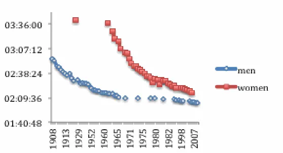
The major issue about producing a chart in Excel is that the ‘x’ axis is not always treated as numeric data. In fact line charts usually treat the ‘x’ axis as categorical data, which is fine for text labels, but may produce unexpected (in this case no recognisable chart) results for numerical data. Consequently if ‘years’ are used for the ‘x’ axis then the only way to get Excel to treat the ‘x’ axis as continuous numeric is to use a scatterplot (Figure 1).
Figure 1. The progression of men and women’s world marathon record times (using the scatterplot function in Excel).
The problem with Figure 1 is that the dates, whilst arranged chronologically, are not uniformly spaced i.e. the distance between 1908 and 1909 is the same for between 1935 and 1953. This will give a distorted view in relation to the actual situation. To get Excel to produce the ‘x’ axis with uniform spacing according to the date then a line chart has to be used where the ‘x’ axis data is formatted as date data. See http://pubs.logicalexpressions.com/Pub0009/LPMArticle.asp?ID=190 for a discussion on this point. A second consideration relates to the data. Figure 1 includes all recorded world records although the Association of Road Racing Statisticians have disputed some of them due to the distance run. For example the 1926 women’s record is suggested to have taken place over a distance of 35.4 km. For this reason the more obvious dubious records (n=5) have been removed from the following charts.
424 | 2012 | ISSUE 2 | VOLUME 7 © 2012 University of Alicante Considering Figure 2 it is evident that the men’s and women’s world records have not progressed in a similar fashion. The linear regression model has been fitted to the data to show how the two lines meet at some point in time (as done by Whipp and Ward, 1992). However when scaling the chart to fit both men’s and women’s world records it is relatively difficult to see the progression of the men’s world records and can lead to false assertions. Consequently the two sets of world records have been charted individually (Figures 3 and 4).
Figure 3. The men’s world marathon record times.
Figure 4. The women’s world marathon record times.
VOLUME 7 | ISSUE 2 | 2012 | 425
So how do we mathematically represent these two different sets of world records? If we consider the women’s records we can see some explanation for why Whipp and Ward used a straight line fit for the data, namely there was a reasonably consistent improvement over time up until the early 90’s when they wrote their paper. However the data now appears to be somewhat curvilinear in that both plots (Figures 3
and 4) are now characterized by three periods where the improvement is decreasing over time. So which type of trend line is a better fit for the world record data? We can test this mathematically but at this point in time it is advisable to consider logic. Logically world record times cannot continue to improve in a linear fashion as at some point in the future the prediction would suggest the world record would be 0 secs, clearly impossible. Therefore a curved line would seem more logical as this implies that there is a limit on the ultimate best performance possible, although we don’t know what this performance is going to be.
Nevill and White (2005) suggested a flattened S shape logistic curve was the best fit for analysing world record times although they used the running speed (m/s) as opposed to the time achieved (Figure 5). Using this curve we might predict that there would be an initial slow improvement, followed by a period of relatively rapid improvement and a final slow rate of improvement.
Figure 5. The progression of men’s running speed for world record marathon times.
The flattened S shape logistic curve as used by Nevill and White (see also Kuper & Sterken, 2008 for a debate and examples on statistical models including the Gompertz curve) provides a fit to the data that suggests that there is a limit to performance as the bottom of the S represents the best performances and the curve approaches some upper limit. Nevill and White (2005) found that the S shaped curve fitted the data well (R2 = 0.974) and calculated the upper limit for running speed in the marathon to be 5.688 m/s, precisely the average running speed of the current world record, set in 2011. Time will tell whether Patrick Makau’s world record, as Nevill and White’s S shaped logistic curve predicted, will never be beaten!
426 | 2012 | ISSUE 2 | VOLUME 7 © 2012 University of Alicante speed and time are the same except for the direction) it appears that the early stages are characterised by relatively large improvements in comparison to the latter stages. This is logical using the law of diminishing returns, which suggests that as performance improves it becomes progressively more difficult to carry on improving (Schmidt and Lee, 2005). Thus we could predict that performance (indeed any form of learning) is characterised by a simple curve (exponential in nature) although the shape of this curve may vary (e.g. logarithmic, polynomial) according to the task difficulty, number of participants, influence of training practices, equipment changes and ergogenic aids. Each of these influences may result in periods of relatively rapid change or lack of change, for example a new training method may result in performance gains additional to expected gains over the time period. Additionally a particularly gifted athlete could improve performance beyond the normal rate of improvement and once that athlete retires a period of catch up takes place where no improvements take place. Hence we might expect deviations in performance from the simple curve but if we consider the evolution of any performance from the first endeavours to the limits of human performance we might imagine that a curve with logarithmic or exponential properties would be fit this data.
An alternative view is given by Nevill and White (2005) who suggest that the period of most rapid improvement occurs later on in the life cycle of a performance improvement. Indeed the running speed data (Figure 5) appears to show a faster rate of improvement than predicted by the simple curve between 1947 and 1967 preceded and followed by periods of slower improvement. This portion of the data therefore fits the flatted S shape curve theory, although the previous simple curve theory also allows for this pattern. The issue with this theoretical perspective is how to explain the relatively slow rate of improvement predicted for the first stages. Nevill and White refer to the amateur regulations which limited the number of athletes competing in the 1900’s. Whilst this is logical for this data it does not explain how the S shaped curve could be applied for other data sets. For example if we consider learning a new skill and tracking the life cycle of the skill development would an S shaped curve fit this data or would a simple curve be more applicable? This paper will consider this question by fitting curves to data related to skill development in Real Tennis. These curves will then be used to try to predict future performance.
VOLUME 7 | ISSUE 2 | 2012 | 427
the skill level of the player. This only works if players play different opponents frequently and inter-club matches take place. For example, if players from one club do not mix with players from other clubs their handicaps will be relative to the players in the club but may be out of sync with players from other clubs. Fortunately Real Tennis has a very advanced Internet database which combines court booking, entering match results and recording of handicaps. Consequently it is very easy to record match details, the handicap permutations are calculated automatically within the software, and hence it is the “norm” rather than the “unusual” that handicap matches are played and recorded. This means that Real Tennis players have a relatively accurate measure of their proficiency in the sport, which is regularly amended to keep accurate, in a similar manner to golf (James, 2007). Handicaps range from -13 to 103 (as of 7 December 2011) with changes to handicap occurring in a consistent way irrespective of the magnitude of the handicap. This results in a linear scale that reflects skill level that can theoretically be used to predict performance over time. This paper will assess the viability of this statement and attempt to determine a viable method for predicting future performance.
MATERIAL AND METHODS
Records of hours and matches played, wins and losses, handicap and world ranking were recorded for one player over a period of 15 months. This player had never played the game at the outset of the data collection although he had both tennis (low senior county standard) and squash (considerable county and national overage experience). Over the data collection period he accumulated 198 hours of on court time (playing matches, training with a partner and solo practice). He started with a handicap of 55, played 101 matches, winning 57.43%, losing 17.82% and ending with a handicap of 29.1.
At the outset of the data collection a prediction was made regarding the progression of this player’s handicap. Taking into account previous profiles of this player’s improvement in performance in golf and squash, but with only a limited knowledge of the structure of the handicap system in Real Tennis, targets were set such that predicted performance improvement would follow a simple curve with logarithmic properties (initial improvement would be greater than later improvements) to achieve a handicap of 15 after three years of play. This curve was calculated by hand without recourse to an equation and so one of the aims of this paper was to assess both the extent to which this curve had been accurate and also whether there was a more scientific method for producing the prediction curve.
RESULTS
428 | 2012 | ISSUE 2 | VOLUME 7 © 2012 University of Alicante
Figure 6. Player’s handicap progress in relation to original targets set.
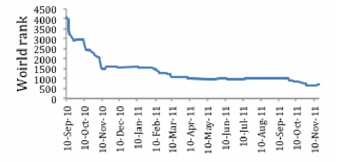
The bi-monthly targets were a relatively gross measure of performance given that records were kept for each day of training/match play. Consequently more in depth analyses were conducted starting with the progress of the player’s world ranking which was plotted on each day that a match was played over the time frame of the study (Figure 7). In line with the handicap data in Figure 3, it seemed that after a period of initial improvement there was a period of no improvement (referred to in the leaning literature as a plateau), followed by another period of improvement, then another plateau before another period of improvement.
Figure 7. Player’s world rank progress over time (line chart in Excel using dates).
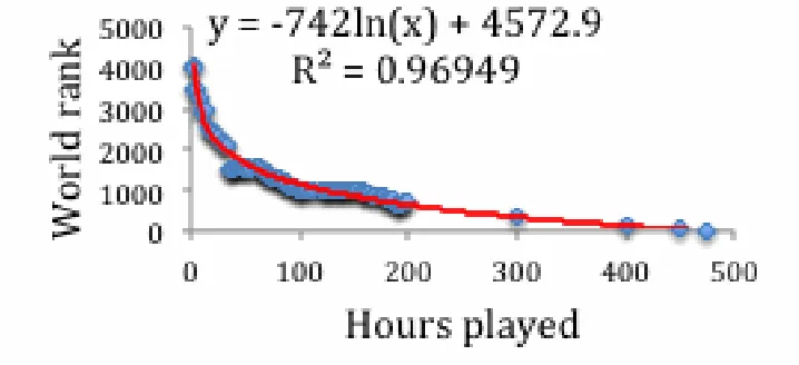
In terms of learning the literature suggests plateaus occur where no improvement is found although in this case it was noticed that the plateaus tended to occur at periods when relatively little Real Tennis was being played. For this reason the world rank information was plotted against the number of hours played (Figure
VOLUME 7 | ISSUE 2 | 2012 | 429
Figure 8. Player’s world rank progress for each hour on court (scatter chart in Excel).
When the world rank data was plotted against the number of court hours the plot (blue dots, Figure 8) appeared to resemble a curve better than when plotted over time. This seems to make more sense as the plot now demonstrates the relationship between performance level (world rank) and hours of practice (hours on court). The best fit curve (R2 = 0.966, red line, Figure 8) was logarithmic in nature, as previously predicted. This was determined using Analyse, Regression, Curve estimation in the IBM® SPSS® Statistics (v. 19) program. The same curve was calculated in Excel (using add trendline and selecting the logarithmic and selecting display equation and R2). A note of caution however, this only works if a scatterplot is used as this correctly uses the ‘x’ axis data as continuous numeric data, if a line chart had been used the calculated equation would have been incorrect.
If we substitute is some values for x (number of hours played) into the equation shown in Figure 8 we find that after 300 hours the world rank is predicted to be 341, 400 hours 127 and after just 474 hours of play this player is predicted to become the number 1 player in the world (Figure 9). This does not seem likely!
430 | 2012 | ISSUE 2 | VOLUME 7 © 2012 University of Alicante The reason for this is not obvious so the world ranking data (accessed from www.realtennisonline.com) was examined in relation to player’s handicaps to see if there was a linear relationship between the two. Figure 10 clearly shows that this is not the case, the curve reflecting the fact that handicaps are relatively normally distributed where most players have handicaps distributed around the average handicap of 55. However, there was a relatively linear relationship over the handicap range for the analysed player (55 to 29) which meant that the prediction (Figure 9) was based on an erroneous premise i.e. the relationship between handicap and world rank was relatively linear throughout the full range of handicaps. Since the regression curve was based solely on the available data the predicted world ranks were wrongly based on a continuous relatively linear improvement in world rank with performance improvement.
Figure 10. World ranking in relation to handicap for Real Tennis.
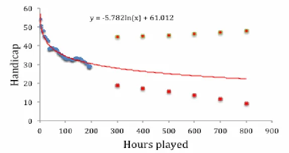
Consequently the handicap data was analysed in a similar manner with an initial plot of handicap against hours played (blue dots, Figure 11) and the line of best fit (red line) calculated in IBM® SPSS® Statistics and plotted in Excel.
VOLUME 7 | ISSUE 2 | 2012 | 431
If we substitute is some values for x (number of hours played) we find that after 300 hours the handicap is predicted to be 28, 400 hours 26 and after 10,000 hours of play this player is predicted to achieve a handicap of 8 (Figure 12).
Figure 12. Player’s predicted handicap progress for each hour on court.
This prediction suggests that after 3 years of play, the original target for this time frame was 15; the player should achieve a handicap of 25, based on 150 hours play per year. This seems more likely than the prediction based on world rank but how accurate is this prediction and how can we assess it?
The prediction is solely based on previous performance and the shape of the curve is based on this data without knowledge of where on the overall performance/learning curve the data fits or whether there have been any periods of unusual improvement or lack of improvement. Consequently the curve could under or over predict future achievement. It may be better, therefore, to give limits for future performance rather than precise estimates. One method for achieving this is to use confidence intervals which IBM® SPSS® Statistics can calculate using the save option.
432 | 2012 | ISSUE 2 | VOLUME 7 © 2012 University of Alicante
DISCUSSION AND CONCLUSIONS
Predicting future performance levels from previous ones would seem to be a useful goal for performance analysts/coaches as this be used as a motivational tool whereby realistic targets for future performance can be set. However all of the predictions in this paper have either been shown to be erroneous or are unlikely to be correct. The original Whipp and Ward (1992) prediction was shown to be inaccurate and the obvious problem with their model was the use of a linear regression line. Whilst this fitted the data reasonably well, predictions based on this model would become more erroneous over time. This model did not consider the limits of human performance and this may be necessary information required to make accurate predictions. Nevill and White (2005) improved on the linear model, using a flattened S shape logistic curve, which enabled them to estimate the limits of human performance. However, the fact that the marathon has already been run at the suggested limit suggests that they under estimated human running potential. This paper analysed some new data to see if some explanations for the difficulty of making accurate predictions could be ascertained.
Handicap and world ranking data was used to represent one player’s skill development in Real tennis. This was an incomplete data set, assuming the player continues to play the game, where the future performance level was unknown, Hence the data resembles the world record data in that both are incomplete records of performance with an unknown final performance level. It was theorised that the progression of the real tennis data would follow a curve with exponential properties. This was based on the law of diminishing returns, which suggests that as performance improves it becomes progressively more difficult to carry on improving (Schmidt and Lee, 2005). This seems logical although the shape of the curve and the magnitude of the limit of performance will depend on the nature of the task and individual differences in terms of innate ability, motivation, practice conditions etc.
When the world rank data was plotted against the number of hours the player had spent on court and a logarithmic curve fitted it was evident that the properties of the curve over estimated the progression of the world rank. The explanation for this is that world rank data is relatively linear over the handicap range for the analysed player (55 to 29) but this linearity does not continue for lower handicaps. Hence the prediction of future world rank performance was not based on the shape of the world rank data (calculated separately using the realtennisonline database) but rather an estimate of what would happen based on how the world rank had progressed in the known data. This is a crucial issue for prediction, how to determine future progression?
VOLUME 7 | ISSUE 2 | 2012 | 433
after 300 hours of play. This is a large range of values that reflects the data collected to this point and further research is necessary to determine how adding more data to the prior performances will affect future predictions.
Prediction has inherent error related to the uncertainty of any future performance. It would seem sensible therefore to produce upper and lower limits for future performance levels using confidence intervals. Confidence intervals can be specified to be relatively certain of successfully predicting future performance by using a high percentage certainty but this will result in a large difference between lower and upper limits. Future studies may wish to determine the optimum trade off between certainty of prediction and acceptable range for lower and upper limits of performance.
REFERENCES
1. JAMES N. The role of notational analysis in soccer coaching. International Journal Sports Science
and Coaching. 2006; 1(2):185-198. doiBack to text]
2. MCGARRY T, FRANKS IM. In search of invariant athletic behaviour in competitive sport systems: an example from championship squash match-play. Journal of Sports Science. 1996; 14:445-456.
doiBack to text]
3. NEVILL AM, WHITE G. Are there limits to running world records? Medicine Science Sports and
Exercise. 2005; 37(10):1785-1788. doiBack to text]
4. SCHMIDT RA, LEE TD. Motor control and learning. A behavioral emphasis. 4th ed. Champaign (IL): Human Kinetics; 2005. [Back to text]
5. WHIPP BJ, WARD SA. Will women soon outrun men? Nature. 1992; 355:25.
doiBack to text]
6. GOMPERTZ B. On the nature of the function expressive of the law of human mortality, and on a new mode of determining life contingencies. Philosophical Transactions of the Royal Society of London. 1825; 115:513-585. [Back to text]
7. HUGHES MD, EVANS S, WELLS J. Establishing normative profiles in performance analysis. International Journal of Performance Analysis in Sport. 2001; 1:1-26. Back to text] 8. KUPER GH, STERKEN E. Modelling the development of world records in running. Statistical
thinking in sports. New York: Chapman and Hall/CRC; 2008. [Back to text]
9. JAMES N. The statistical analysis of golf performance. Annual Review of Golf Coaching. 2007; 231-248Back to text]
10. JAMES N, JONES NMP, MELLALIEU SD. The development of position-specific performance indicators in professional rugby union. Journal of Sports Sciences. 2005; 23(1):63-72.
doiBack to text]
11. JONES NMP, JAMES N, MELLALIEU SD. An objective method for depicting team performance in elite professional rugby union. Journal of Sports Sciences. 2008; 26(7):691-700.
doiBack to text]