A comparative Experimental Study of Heuristics for Multi Objective Disassembly Planning

(1)

167705-2929-IJMME-IJENS © October 2016 IJENS

A comparative Experimental Study of Heuristics for

Multi Objective Disassembly Planning

P. Marchionna, S. Paradiso, G. Percoco,

Politecnico di Bari, Italy

Abstract— This paper is a contribution towards the identification of the best optimization algorithm to detect convenient disassembly sequences for end-of-life industrial products. Three methodologies are proposed for comparison: Artificial Colony Optimization, Genetic Algorithms and Simulated Annealing. These algorithms are compared using case studies including partial and full disassembly.

Index Term— Artificial Colony Optimization, Disassembly Sequence, Genetic Algorithms, Simulated Annealing.

I. INTRODUCTION

The reduction of waste saves money and generates profits [1]. Moreover several regulations, such as the Waste Electrical and Electronic Equipment (WEEE) Directive, Restriction of the use of certain Hazardous Substances (RoHS) Directive, End-of-life Vehicle (ELV) Directive, etc., are compelling manufacturers to deal with end of life (EoL) products in an environmentally-friendly way.

The EoL recovery strategy is important and several aspects must be considered such as: recovery option selection and disassembly sequence planning. In literature, the main recovery options are considered to be (i) remanufacturing, (ii) reuse, (iii) recycling [2].

In this context disassembly is the main involved process and tends to be costly, because of the actual and continuously increasing complexity and high variety of products. As a consequence, disassembly process planning is very important in minimizing maintenance cost and recovering end-of-life products.

In [3] disassembly is classified into complete, target selective and partial disassembly. In industrial practice, complete disassembly is not cost effective and in many cases not feasible. Selective disassembly consists in choosing a specific component as target to find the optimal disassembly sequence to extract it. Complete and selective disassembly can be considered shortest path problems or particular cases of the more general partial disassembly. A deeper disassembly may reduce the return on the EoL product, due to expensive operations. As a consequence partial disassembly has become important for research [4], [5].

The purpose of this paper is to compare several heuristic strategies to optimize the disassembly cost, considering the cases that involve partial disassembly as best disassembly strategy. Three well known heuristic strategies, namely Artificial Colony Optimization (ACO), Genetic Algorithms (GA) and Simulated Annealing (SA), have been implemented in the present paper, to achieve optimal or nearly optimal

recovery options and disassembly planning, based on a cost function proposed in literature.

This paper is organized as follows: section II reviews the most relevant previous research; section III describes the mathematical model and the algorithms implemented in the present paper; section IV shows and describes the case studies, the first with ten components and the second, composed by 25 components, studied in two versions: when a full disassembly leads to optimization and when a partial disassembly is the optimal solution; in Section V the results are shown and in section VI the results are discussed; in section VII the conclusions are exposed while section VIII is the appendix that includes the interference matrices used for the products with 25 components.

II. LITERATURE REVIEW

Research on Disassembly process planning has been performed on various aspects, such as the analysis of the optimal level of disassembly, i.e. the level that makes it advantageous to bear the costs of the process itself, since for each component or sub-assembly there is a different end-of-life perspective. In this context the disassembly sequence is crucial having a strong impact on efficiency and cost, the complexity of the task increases with the complexity of the product. As regards environmental protection, the aim of disassembly can be summarized as follows: obtaining parts, components and subassemblies for reuse in new products; recovery of recyclable materials; removal of hazardous or toxic materials; access to parts or components that may be subject to service operations (repair, maintenance and diagnostics). [6]

In literature many researchers focused on complete disassembly planning for EoL products through approaches including Petri Net [7], Linear Programming [8], Genetic Algorithms [9] [10], Particle Swarm Optimization (PSO) [11], Ant Colony Optimization and Artificial Bee Colony Optimization [12]. More recently a Tabu Search implementation for Genetic Algorithms has been proposed [12], to improve convergence to the optimal solution. Some relevant examples of papers about selective disassembly are [13], that proposed wave propagations, to topologically order components to find a feasible sequence and [14] that determined an optimal sequence by geometric reasoning approach. Since geometric approaches impose a computing time that exponentially increases with the complexity of the problem, intelligent optimization methods, such as GA [15] and ACO [16], have been implemented for selective disassembly planning.

(2)

considering disassembly revenue, environmental impact and disassembly feasibility is proposed.

III.PROBLEM DESCRIPTIONAND RESEARCH MODEL In this paper the author have compared three of the most effective heuristic techniques to solve the disassembly sequence problem simultaneously optimizing economic costs and environmental costs through the optimization of the multiobjective function proposed in [20], with the assumptions used in [21]. For the sake of brevity the function is not described in this paper, being shown in [20] and [21].

The product to be disassembled is considered as a set of components. Considering a generic collection of n components, it is possible to number them from 1 to n. The following information can be associated with each item and are considered in the cost function shown in [20] and [21]: (i) time of disassembly, required to remove the component, it can be hypothesized also with the help of specialized data-bases; (ii) Cost of disassembly, it depends on the chosen disassembly sequence; (iii) Environmental impact, that quantifies environmental effects associated to the end-of-life phase of each component.

As regards the feasibility of the sequences, the disassembly relationships can be graphically represented by the Disassembly Precedence Graph (DPG), where a node represents a component and an arrow line couples two nodes to indicate the disassembly precedence relationship. In this paper the DPG is converted into a Disassembly Precedence Matrix (DPM), where DPM = [DPMij ] with j = 1, 2, …, n

and i = 1, 2, …, n. DPMij = disassembly time of the

component i if the ith component prevents removal of the j-th component, otherwise DPMij = 0.

A. Assumptions

To solve the problem of disassembly planning, the following assumptions have been made by the authors:

- Disassembly sequence is denoted as the serial order of parts removal. The optimal disassembly directions and disassembly precedence are deterministic, being the status of EoL components predictable. Each component is the minimum disassembly unit and can be totally recyclable or not recyclable at all.

- Remanufacturing and reuse are not considered in this study. The analysis is focused on the comparison of several heuristics and the inclusion of both these possibilities would not change the formulation of the problem, nor the capability of the algorithms to achieve optimal or suboptimal solutions.

- Economic information (e.g. recovery revenue, reprocess cost), process information (e.g. disassembly method, disassembly time) are hypothesized after interviews involving specialized companies, these data are easy to be retrieved if a Product Lifecycle Management software is available.

B. Genetic Algorithms

The GA chromosome used in this study is a vector c=(c1,

c2, c3, …, cn) where (c1, c2, c3, …, cn) is a permutation of the

integers (1,2,3,…n).

The crossover operator chosen was the well-known simple formulation, while as regards mutation, two mutation

operators were used: namely mutation 1, consisting in replacing the j-th gene of the population with the next gene k in case the gene, before the j-th, also ensures the recycling of the component k. This mutation guarantees that the sequence does not change the number of recyclable components, but there is a change of the cost of disassembly, due to the variation of disassembly times.

The mutation 2 operation is to replace the j-th gene of the population with k-th if the gene, before the j-th, ensures the recycling of the component j but does not guarantee the recycling of the component k. This type of mutation is to assess those sequence changes that modify the number of recycled components, varying the disassembly cost.

The GA employed was set with a population of n3/2 individuals and 3n3/2 individuals as a result of the reproduction stage. The stop criterion was obtained setting the maximum number of iterations without improvement of the fitness function.

C. Simulated Annealing

The Simulated Annealing is a strategy used to solve optimization problems. This process aims to find a global minimum in the presence of multiple local minima. The concept of annealing is derived from the metals science, where it is used to describe the process of elimination of lattice defects, using a heating procedure followed by a slow cooling.

Simulated Annealing algorithm progresses through the following steps:

1- definition of initial population and computation of the energy of each solution member

2- raising the population's energy, through a random perturbation. High probability in replacing the members of the initial population with perturbed ones, even if worst, ensure the raising of energy and a good exploration of the search space.

3- Slow reduction of energy that progressively reduces the ability to replace a solution with a worse one.

The parameter settings involve:

- the initial population constituted of n individuals, being n the number of components of the product

- the energy T of a solution is the value of the cost function - the probability P to accept the worst solution of the expression (e ΔT/KBT )Number of Cycles where ΔT is the difference in cost between perturbed and initial solution and KBT is the Boltzmann constant.

Two different types of perturbation are used, the first one takes place for the first n-1 cycles, working as follows: at the ith cycle the probability that every possible j follows i is estimated through the DPM and the jth component is detected stochastically. The second perturbation is equal to the mutation 1 of the GA.

Stopping criteria set for the algorithm are: maximum number of iteration cycles or convergence after a maximum number of cycles with no decrease of the cost of disassembly.

D. Ant Colony Optimization

(3)

167705-2929-IJMME-IJENS © October 2016 IJENS 1- Random Generation of a population of sequences

2- Identifying the best locations

3- Pheromone release in proportion to the goodness of the solution

4- Generation of a new population of sequences by a stochastic local rule, which increases the amount of pheromone.

This rule stipulates to evaluate the average profitability of the population. Only a portion of solutions continues in the execution of the algorithm, namely those in line with the average of the colony, the remaining part are eventually deleted according to the scheme:

- Ant profitability > 0.9 * average profitability → 80% chance of eliminating the Ant

- Ant profitability < 0.8 * average profitability → 80% chance of eliminating the Ant

- 0.8 * average profitability < Ant profitability < 0.9 * average profitability → 20% chance of eliminating the Ant

- 0.9 * average profitability < Ant profitability < 0.95 * average profitability → 2% chance of eliminating the Ant

- 0.95 * average profitability < Ant profitability → the Ant certainly survives.

At the end of the selection process, a new population constituted exclusively from solutions (surviving ants) that will continue the optimization process.

Inputs and outputs are the same as the Genetic algorithm. Stopping criteria set for the algorithm are: maximum number of iteration cycles or convergence after a maximum number of cycles with no decrease of the cost of disassembly.

IV.CASE STUDIES

All the case studies have been evaluated under the hypotheses of labour cost Cmdo=6.25 €/h, setup time d= 5 sec,

disposal cost CS= 0.127 €/kg, steel recycling profit 84.2 €/t,

plastics recycling profit 185.5 €/t.

A. Product 1

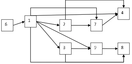
The first case study is composed of ten components, with a disassembly network shown in Fig. 1. The components number 5 and number 10 are not included in the graph because of the difficulty of representation, assuming that number 5 can be disassembled after any of the components, while number 10 can be disassembled only as the last component.

Fig. 1. Flow disassembly network for the first product

The main data used for this product are shown in Table I, where the profit from recycling and weight are shown for each

component, and Table II, where the sequence dependent disassembly times are hypothesized.

Table 1

Profit from recycling and weight for each component

Compon ent

Profit from recycling (€/Kg)

Weight (Kg)

1 0.0842 1.05

2 0.0842 0.12

3 0.0842 0.7

4 0.0842 0.936

5 0.0842 0.76

6 0.1855 0.34

7 0.0842 1.8

8 0.1855 0.6

9 0.0842 0.24

10 0.0842 0.3

B. Product 2

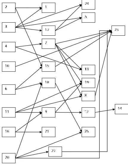
The second product is a virtual product that have been tested in the literature [22]. The data have been adapted by the authors.

The data available from the literature for this product are the precedence matrix and the volume of the components. These data led to the precedence graph shown in Fig. 2, while the disassembly times were hypothesized and reported in Table VI and VII, reported in the appendix.

The following data have been assumed:

(4)

Table II

Disassembly time matrix for the first product

16, 18, 22, 23, 24 are considered made of plastic material while the remaining are made of steel.

-the weights of each component, determined by volume and material

-the setup required, a single setup has been considered for simplicity: the introduction of a new setup would not affect the capability of algorithms

-profits from recycling, determined by composition material

-the labour cost

-disassembly times: two different time matrices have been hypothesized for this product, the first one is featured for complete disassembly, the second one for partial disassembly.

As well as product 1 the disposal profit for steel parts was 0.0842 €/Kg, while for plastic parts was 0.1855 (€/Kg).

The Disassembly time matrix used for total and partial disassembly are reported in the Appendix (Table VI and Table VII) for the sake of clarity.

Fig. 2. Flow disassembly network for the first product

V. RESULTS

Each product was analysed through 20 runs for each kind of algorithm, exploiting the three product configurations explained above, one configuration for Product 1 and two different configurations for Product 2.

A. Product 1

As regards the first product, constituted of 10 components, in Fig. 3 the average function versus the number of iterations for the first product is shown.

Fig. 3. Optimization Function vs Iterations for the first product

Dismantling time (sec) Setup

Comp. 1 2 3 4 5 6 7 8 9 10

1 0 52 62 0 0 0 0 0 0 0 1

2 0 0 62 0 0 0 71 29 68 0 0

3 0 52 0 53 0 0 71 0 68 0 1

4 0 0 62 0 33 0 0 29 62 0 1

5 0 0 0 0 0 0 0 0 0 35 0

6 85 0 0 0 0 27 0 0 0 0 1

7 0 0 62 0 0 0 0 29 65 0 1

8 0 52 0 63 0 0 64 0 0 0 0

9 0 52 0 63 0 0 64 29 0 0 1

(5)

167705-2929-IJMME-IJENS © October 2016 IJENS This graph is obtained averaging for each algorithm and each

iteration the value of the fitness value in each run. When a run is terminated because of the intervention of the stop criteria, it is not considered in the average computation.

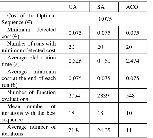
In Table III a synoptic table of the results is shown, including all the main results achieved by the algorithms, such as the cost of the best sequence computed with deterministic methods; the minimum cost detected by the heuristics, the elaboration time averaged over the 20 runs for each algorithm, the average minimum cost computed over the 20 runs for each heuristic, the number of evaluation of the optimization function, the average number of iterations after the detection of the best sequence before the intervention of the stop criteria, the average number of iterations before algorithms stop.

Table III

Synoptic table of the results for Product 1

B.Product 2 -Full Disassembly

In Fig. 4 the average function versus the number of iterations for the second product is shown, while Table IV summarizes the performances of each algorithm, under the hypothesis that the disassembly matrix is the one shown in Table VI (Appendix).

Fig. 4. Optimization Function vs Iterations for the second product in case of partial disassembly

Table IV

Time matrix for the second product-full disassembly

C.Product 2 -Partial Disassembly

In Fig. 5 the average function versus the number of iterations for the second product is shown, in the case that the disassembly matrix is that shown in Table VII (Appendix), while the synoptic table is reported in Table V. In both Table IV and Table V the cost of the optimal sequence is not specified, being too heavy the deterministic computation.

GA SA ACO

Cost of the Optimal

Sequence (€) 0,075

Minimum detected

cost (€) 0,075 0,075 0,075

Number of runs with

minimum detected cost 20 20 20

Average elaboration

time (s) 0,326 0,160 2,474

Average minimum cost at the end of each run (€)

0,075 0,075 0,075

Number of function

evaluations 2054 2339 548

Mean number of iterations with the best sequence

18 18 10

Average number of

iterations 21,8 24,05 11

GA SA ACO

Cost of the Optimal

Sequence (€) -

Minimum detected

cost (€) 0,015 0,024 0,033

Number of runs with

minimum detected cost 1 1 1

Average elaboration

time (s) 9,093 9,617 285,1

0,021 0,032 0,042

Number of fitness

evaluations 31859 43631 9807

15,6 8,2 20,75

Average number of

(6)

Fig. 5. Optimization Function vs Iterations for the second product in case of partial disassembly

Table V

Time matrix for the second product partial disassembly

GA SA ACO

Cost of the Optimal

Sequence (€) -

Minimum detected

cost (€) 0,057 0,062 0,078

Number of runs

with minimum

detected cost

1 1 1

Average elaboration

time (s) 7,498 8,483 1192

0,065 0,072 0,083

Number of fitness

evaluations 25520 41760 38554

14,55 6,8 49,05

Average number of

iterations 68,9 68,2 97,45

VI.DISCUSSION OF RESULTS

The three graphs put in evidence how the GA is the best algorithm in minimizing the fitness function. The SA performs also well while the worst is ACO.

Analysing the Tables III, IV, V it is possible to make further considerations. The cost of the best sequence computed with a deterministic method is available only for the Product 1, since the number of components is low; this cost is fully targeted by the three algorithms. As regards Product 2 the deterministic computation of the cost would require a very high computation time and is not performed. The minimum cost was found by GA as mentioned before but it is important to underline that the three algorithms reached the best value only in one run The elaboration time are very low both for GA and SA, while ACO had a bad performance.

With regard to the average minimum cost, computed over the 20 runs for each heuristic, the GA is always the best performing, followed by SA. The tables show also the number of evaluations of the optimization function for each algorithm. The ACO appears to have very good performances but it must be considered the worst in finding minima and that in the case of Product 2, full disassembly, it is evident a premature convergence.

The average number of iterations, after the detection of the best sequence, before the intervention of the stop criteria gives information about the validity of the stop criteria.

The results of the average number of iterations confirm a good performance of GA and SA.

VII.CONCLUSIONS

(7)

Table VI

Disassembly time matrix used for total disassembly for the product 2

Comp. 1 2 3 4 5 6 7 8 9 10 11 12 13 14 15 16 17 18 19 20 21 22 23 24 25

1 0 2 2 3 2 2 3 2 3 3 3 3 3 2 2 3 3 3 2 3 3 2 3 3 2

2 0 5 5 8 4 8 9 6 7 8 5 8 7 9 0 5 8 6 11 8 8 5 7 6 10

3 0 4 3 3 0 2 2 5 2 3 3 2 3 2 5 4 0 2 4 5 3 4 2 0 4

4 15 19 19 16 21 19 0 15 16 11 21 16 0 21 19 11 11 15 18 15 17 11 18 21 18

5 2 2 0 2 0 2 2 2 2 1 2 2 1 2 2 2 2 2 2 2 2 2 2 2 2

6 3 3 3 3 3 3 3 4 3 4 4 4 3 3 0 3 3 0 3 3 3 3 1 4 4

7 3 4 3 2 3 3 0 0 2 3 3 4 0 2 4 4 2 4 0 1 4 3 0 3 3

8 5 8 5 0 5 6 2 0 6 6 4 4 6 4 7 4 7 5 6 5 9 5 0 4 4

9 12 13 12 12 11 18 16 14 0 16 14 0 15 20 10 9 21 17 0 18 18 20 12 16 19

10 1 1 1 1 1 1 1 1 2 1 1 1 1 2 2 1 1 1 1 1 1 1 0 1 1

11 8 6 3 6 6 7 7 0 0 7 6 7 8 6 4 5 5 7 0 6 6 6 8 4 5

12 2 2 3 1 2 2 2 2 2 1 0 0 2 0 2 0 2 2 2 1 1 1 2 2 2

13 7 7 8 0 8 9 10 11 6 9 8 8 0 6 8 7 6 7 4 7 8 5 7 8 6

14 4 4 5 5 5 5 3 6 0 6 0 5 5 0 4 0 5 6 4 5 5 6 5 7 6

15 5 5 7 4 5 6 3 6 5 6 5 5 7 6 0 5 6 3 3 6 6 6 0 4 5

16 1 2 1 2 2 2 2 1 0 1 1 1 1 2 2 1 1 2 2 1 1 1 2 1 1

17 3 4 3 3 0 3 5 4 2 4 4 3 4 4 4 3 0 4 4 3 0 5 3 0 4

18 5 3 3 5 5 5 6 6 6 6 5 5 6 5 5 6 6 0 3 5 6 4 4 4 0

19 32 32 19 0 24 23 31 23 18 33 0 26 25 31 25 28 20 28 0 25 28 28 22 27 24

20 6 6 8 9 7 11 7 5 8 7 9 5 6 11 7 5 7 0 7 6 6 0 0 6 0

21 3 4 3 3 3 3 4 3 2 4 4 4 4 3 3 2 3 4 3 4 0 5 4 4 4

22 2 2 1 2 1 2 1 1 1 1 2 1 2 2 2 2 2 1 2 2 2 0 0 1 1

23 2 0 3 0 2 0 0 2 1 3 0 1 1 3 3 1 2 2 3 0 2 1 0 2 2

24 3 3 0 4 2 4 5 4 2 3 4 3 4 4 3 3 3 4 3 3 4 3 3 0 3

25 10 10 8 10 12 0 12 12 14 12 9 10 12 11 9 11 9 11 9 0 9 9 10 12 0

(8)

Table VII

Disassembly time matrix used for partial disassembly

Comp 1 2 3 4 5 6 7 8 9 10 11 12 13 14 15 16 17 18 19 20 21 22 23 24 25

1 0 2 2 3 2 2 3 2 3 3 3 3 3 2 2 3 3 3 2 3 3 2 3 3 2

2 0 5 5 8 4 8 9 6 7 8 5 8 7 9 0 5 8 6 11 8 8 5 7 6 10

3 0 4 3 3 0 2 2 5 2 3 3 2 3 2 5 4 0 2 4 5 3 4 2 0 4

4 15 19 19 16 21 19 0 15 16 11 21 16 0 21 19 11 11 15 18 15 17 11 18 21 18

5 3 4 0 4 0 4 4 3 4 4 4 4 4 4 4 4 4 3 4 4 4 4 5 4 4

6 3 3 3 3 3 3 3 4 3 4 4 4 3 3 0 3 3 0 3 3 3 3 1 4 4

7 4 4 3 4 3 4 4 0 5 3 3 4 0 5 4 5 4 3 0 5 4 4 0 5 6

8 12 14 13 0 12 9 8 0 14 11 10 13 11 10 10 11 10 10 15 9 10 12 0 13 13

9 12 13 12 12 11 18 16 14 0 16 14 0 15 20 10 9 21 17 0 18 18 20 12 16 19

10 1 1 1 1 1 1 1 1 2 1 1 1 1 2 2 1 1 1 1 1 1 1 0 1 1

11 8 6 3 6 6 7 7 0 0 7 6 7 8 6 4 5 5 7 0 6 6 6 8 4 5

12 3 2 3 2 3 3 2 2 3 2 0 0 2 0 3 0 2 3 3 3 3 3 2 2 4

13 7 7 8 0 8 9 10 11 6 9 8 8 0 6 8 7 6 7 4 7 8 5 7 8 6

14 4 4 5 5 5 5 3 6 0 6 0 5 5 0 4 0 5 6 4 5 5 6 5 7 6

15 5 5 7 4 5 6 3 6 5 6 5 5 7 6 0 5 6 3 3 6 6 6 0 4 5

16 1 2 1 2 2 2 2 1 0 1 1 1 1 2 2 1 1 2 2 1 1 1 2 1 1

17 3 4 3 3 0 3 5 4 2 4 4 3 4 4 4 3 0 4 4 3 0 5 3 0 4

18 5 3 3 5 5 5 6 6 6 6 5 5 6 5 5 6 6 0 3 5 6 4 4 4 0

19 47 49 42 0 34 49 45 45 41 48 0 45 43 37 45 47 44 38 0 40 45 40 46 42 34

20 6 6 8 9 7 11 7 5 8 7 9 5 6 11 7 5 7 0 7 6 6 0 0 6 0

21 3 4 3 3 3 3 4 3 2 4 4 4 4 3 3 2 3 4 3 4 0 5 4 4 4

22 2 3 2 2 3 2 2 2 3 3 3 3 2 3 3 2 3 3 3 2 2 0 0 2 3

23 7 0 6 0 6 0 0 7 7 5 0 6 6 6 6 5 8 6 6 0 7 6 0 6 6

24 3 3 0 4 2 4 5 4 2 3 4 3 4 4 3 3 3 4 3 3 4 3 3 0 3

(9)

[1] S. C. Lee and L. H. Shih, “A novel heuristic approach to determine compromise management for end-of-life electronic products,” J. Oper. Res. Soc., vol. 63, no. 5, pp. 606–619, Jul. 2011.

[2] A. Desai and A. Mital, “Evaluation of disassemblability to enable design for disassembly in mass production,” Int. J. Ind. Ergon., vol. 32, no. 4, pp. 265–281, Oct. 2003.

[3] J. L. Rickli and J. A. Camelio, “Multi-objective partial disassembly optimization based on sequence feasibility,” J. Manuf. Syst., vol. 32, no. 1, pp. 281–293, Jan. 2013.

[4] S. G. Lee, S. W. Lye, and M. K. Khoo, “A Multi-Objective Methodology for Evaluating Product End-of-Life Options and Disassembly,” Int. J. Adv. Manuf. Technol., vol. 18, no. 2, pp. 148–156, Jul. 2001.

[5] X. Q. Shi, L. J. Huang, and H. Wang, “A Multi-Agent System for Remanufacturing of End-of-Life Products,” Adv. Mater. Res., vol. 655–657, pp. 2025–2032, Jan. 2013.

[6] A. J. D. Lambert, “Optimal disassembly of complex products,” Int. J. Prod. Res., vol. 35, no. 9, pp. 2509–2523, 1997. [7] K. E. Moore, A. Güngör, and S. M. Gupta, “Petri net approach

to disassembly process planning for products with complex AND/OR precedence relationships,” Eur. J. Oper. Res., vol. 135, no. 2, pp. 428–449, Dec. 2001.

[8] A. GÜngÖr and S. M. Gupta, “Disassembly sequence plan generation using a branch-and-bound algorithm,” Int. J. Prod. Res., vol. 39, no. 3, pp. 481–509, Jan. 2001.

[9] W. Hui, X. Dong, and D. Guanghong, “A genetic algorithm for product disassembly sequence planning,” Neurocomputing, vol. 71, no. 13–15, pp. 2720–2726, Aug. 2008.

[10] L. M. Galantucci, G. Percoco, and R. Spina, “Assembly and disassembly planning by using Fuzzy Logic & Genetic algorithms,” Int. J. Adv. Robot. Syst., vol. 1, no. 1, pp. 67–74, 2004.

[11] W.-C. Yeh, “Simplified swarm optimization in disassembly sequencing problems with learning effects,” Comput. Oper. Res., vol. 39, no. 9, pp. 2168–2177, Sep. 2012.

[12] M. Alshibli, A. El Sayed, E. Kongar, T. M. Sobh, and S. M. Gupta, “Disassembly Sequencing Using Tabu Search,” J. Intell. Robot. Syst., vol. 82, no. 1, pp. 69–79, Oct. 2015.

[13] H. Srinivasan, R. Figueroa, and R. Gadh, “Selective disassembly for virtual prototyping as applied to de-manufacturing,” Robot. Comput. Integr. Manuf., vol. 15, no. 3, pp. 231–245, 1999.

[14] S. Kara, P. Pornprasitpol, and H. Kaebernick, “A selective disassembly methodology for end‐of‐ life products,” Assem. Autom., vol. 25, no. 2, pp. 124–134, Jun. 2005.

[15] T. F. Go, D. A. Wahab, M. N. A. Rahman, R. Ramli, and A. Hussain, “Genetically optimised disassembly sequence for automotive component reuse,” Expert Syst. Appl., vol. 39, no. 5, pp. 5409–5417, Apr. 2012.

[16] X. Liu, G. Peng, X. Liu, and Y. Hou, “Disassembly sequence planning approach for product virtual maintenance based on improved max–min ant system,” Int. J. Adv. Manuf. Technol., vol. 59, no. 5–8, pp. 829–839, Aug. 2011.

[17] E. Zussman and M. Zhou, “A methodology for modeling and adaptive planning of disassembly processes,” IEEE Trans. Robot. Autom., vol. 15, no. 1, pp. 190–194, 1999.

[18] D. E. Grochowski and Y. Tang, “A machine learning approach for optimal disassembly planning,” Int. J. Comput. Integr. Manuf., vol. 22, no. 4, pp. 374–383, Apr. 2009.

[19] E. Kongar and S. M. Gupta, “Disassembly sequencing using genetic algorithm,” Int. J. Adv. Manuf. Technol., vol. 30, no. 5– 6, pp. 497–506, Dec. 2005.

[20] F. Giudice and G. Fargione, “Disassembly planning of mechanical systems for service and recovery: a genetic algorithms based approach,” J. Intell. Manuf., vol. 18, no. 3, pp. 313–329, Jul. 2007.

[21] G. Percoco and M. Diella, “Preliminary evaluation of artificial bee colony algorithm when applied to multi objective partial disassembly planning,” Res. J. Appl. Sci. Eng. Technol., vol. 6, no. 17, pp. 3234–3243, 2013.