University of Pennsylvania
ScholarlyCommons
Publicly Accessible Penn Dissertations
1-1-2016
Control Theoretic Analysis of Human Brain
Networks
Shi Gu
University of Pennsylvania, gus@sas.upenn.edu
Follow this and additional works at:
http://repository.upenn.edu/edissertations
Part of the
Applied Mathematics Commons,
Biomedical Commons, and the
Neuroscience and
Neurobiology Commons
This paper is posted at ScholarlyCommons.http://repository.upenn.edu/edissertations/1751 For more information, please contactlibraryrepository@pobox.upenn.edu.
Recommended Citation
Gu, Shi, "Control Theoretic Analysis of Human Brain Networks" (2016).Publicly Accessible Penn Dissertations. 1751.
Control Theoretic Analysis of Human Brain Networks
Abstract
The brain is a complex system with complicated structures and entangled dynamics. Among the various approaches to investigating the brain's mechanics, the graphical method provides a successful framework for understanding the topology of both the
structural and functional networks, and discovering efficient diagnostic biomarkers for cognitive behaviors, brain disorders and diseases. Yet it cannot explain how the structure affects the functionality and how the brain tunes its transition among multiple states to manipulate the cognitive control. In my dissertation, I propose a novel framework of modeling the mechanics of the cognitive control, which involves in applying control theory to analyzing the brain networks and conceptually connecting the cognitive control with the engineering control. First, I examine the energy distribution among different states via combining the energetic and structural constraints of the brain's state transition in a free energy model, where the interaction between regions is explicitly informed by structural connectivity. This work enables the possibility of
achieving a whole view of the brain's energy landscape and preliminarily indicates the feasibility of control theory to model the dynamics of cognitive control. In the following work, I exploit the network control theory to address two questions about how the large-scale circuitry of the human brain constrains its dynamics. First, is the human brain theoretically controllable? Second, which areas of the brain are most influential in
constraining or facilitating changes in brain state trajectories? Further, I seek to examine the structural effect on the control actions through solving the optimal control problem under different boundary conditions. I quantify the efficiency of regions in terms of the energy cost for the brain state transition from the default mode to task modes. This analysis is extended to the perturbation analysis of trajectories and is applied to the comparison between the group with mild traumatic brain injury(mTBI) and the healthy group. My research is the first to demonstrate how control theory can be used to analyze human brain networks.
Degree Type
Dissertation
Degree Name
Doctor of Philosophy (PhD)
Graduate Group
Applied Mathematics
First Advisor
Danielle S. Bassett
Keywords
brain, cognitive control, connectivity, controllability, dynamics, energy landscape
Subject Categories
CONTROL THEORETIC ANALYSIS OF HUMAN BRAIN NETWORKS
Shi Gu
A DISSERTATION
in
Applied Mathematics and Computational Science
Presented to the Faculties of the University of Pennsylvania
in
Partial Fulfillment of the Requirements for the
Degree of Doctor of Philosophy
2016
Supervisor of Dissertation
Danielle S. Bassett, Associate Professor of Bioengineering
Graduate Group Chairperson
Charles L. Epstein, Thomas A. Scott Professor of Mathematics
Dissertation Committee
Danielle S. Bassett, Associate Professor of Bioengineering
Fabio Pasqualetti, Assistant Professor of Mechanical Engineering
James C. Gee, Associate Professor of Radiologic Science in Radiology
CONTROL THEORETIC ANALYSIS OF HUMAN BRAIN NETWORKS
c
COPYRIGHT
2016
Shi Gu
This work is licensed under the
Creative Commons Attribution
NonCommercial-ShareAlike 3.0
License
To view a copy of this license, visit
ACKNOWLEDGEMENT
I would like to first thank my parents who support me consistently and unreservedly from
my birth to now. Their back-up and trust offer me the courage and determination along
the journey of life.
I would like to give my special thanks to my advisor Dr. Danielle S. Bassett. Her insightful
instruction directs my exploration in the filed of network neuroscience during my PhD
period.
I would also like to give many thanks to all my committees, colleagues, collaborators, course
professors, and friends for their kind helps in both academia and life.
I also appreciate it sincerely for the financial support from the program of Applied
Mathe-matics and Computational Science, School of Arts and Science and National Science
ABSTRACT
CONTROL THEORETIC ANALYSIS OF HUMAN BRAIN NETWORKS
Shi Gu
Danielle S. Bassett
The brain is a complex system with complicated structures and entangled dynamics. Among
the various approaches to investigating the brain’s mechanics, the graphical method
pro-vides a successful framework for understanding the topology of both the structural and
functional networks, and discovering efficient diagnostic biomarkers for cognitive behaviors,
brain disorders and diseases. Yet it cannot explain how the structure affects the
functional-ity and how the brain tunes its transition among multiple states to manipulate the cognitive
control. In my dissertation, I propose a novel framework of modeling the mechanics of the
cognitive control, which involves in applying control theory to analyzing the brain networks
and conceptually connecting the cognitive control with the engineering control. First, I
examine the energy distribution among different states via combining the energetic and
structural constraints of the brain’s state transition in a free energy model, where the
inter-action between regions is explicitly informed by structural connectivity. This work enables
the possibility of achieving a whole view of the brain’s energy landscape and preliminarily
indicates the feasibility of control theory to model the dynamics of cognitive control. In the
following work, I exploit the network control theory to address two questions about how
the large-scale circuitry of the human brain constrains its dynamics. First, is the human
brain theoretically controllable? Second, which areas of the brain are most influential in
constraining or facilitating changes in brain state trajectories? Further, I seek to examine
the structural effect on the control actions through solving the optimal control problem
under different boundary conditions. I quantify the efficiency of regions in terms of the
en-ergy cost for the brain state transition from the default mode to task modes. This analysis
between the group with mild traumatic brain injury(mTBI) and the healthy group. My
research is the first to demonstrate how control theory can be used to analyze human brain
TABLE OF CONTENTS
ACKNOWLEDGEMENT . . . iv
ABSTRACT . . . v
LIST OF TABLES . . . xi
LIST OF ILLUSTRATIONS . . . xxiii
PREFACE . . . 1
CHAPTER 1 : Introduction . . . 1
1.1 What is a brain network? . . . 1
1.2 Why should we use the control theory to view the brain network? . . . 3
1.3 Mathematical concepts . . . 4
1.3.1 Network Measures . . . 4
1.3.2 Controllability Settings . . . 8
1.4 Contribution of my works . . . 10
CHAPTER 2 : The Landscape of Neurophysiological Activity Implicit in Brain Network Structure . . . 11
2.1 Introduction . . . 11
2.2 Models and Materials . . . 15
2.2.1 Human DSI Data Acquisition and Preprocessing . . . 15
2.2.2 Structural Network Construction . . . 15
2.2.3 Resting state fMRI data . . . 17
2.2.4 Defining an Energy Landscape. . . 18
2.2.5 Discovering Local Minima. . . 19
2.2.7 Activation Rates . . . 22
2.2.8 Utilization Energies . . . 22
2.2.9 Permutation Tests for State Association . . . 23
2.2.10 Predicted Functional Connectivity . . . 24
2.3 Results . . . 24
2.3.1 Local Minima in the Brain’s Energy Landscape . . . 24
2.3.2 Activation Rates of Cognitive Systems . . . 27
2.3.3 Activation Rates of Cognitive Systems . . . 28
2.3.4 Relating Predicted Activation Rates to Rates Observed in Functional Neuroimaging Data . . . 33
2.4 Discussion . . . 38
2.4.1 The Role of Activation vs. Connectivity in Understanding Brain Dy-namics . . . 38
2.4.2 Co-activation Architecture . . . 39
2.4.3 Critical Importance of Energy Constraints . . . 40
2.4.4 Methodological Considerations . . . 40
2.5 Conclusion . . . 41
CHAPTER 3 : Controllability of Structural Brain Networks . . . 43
3.1 Introduction . . . 43
3.2 Mathematical Models . . . 46
3.2.1 Network Control Theory . . . 46
3.2.2 Dynamic Model of Neural Processes . . . 47
3.2.3 Network Controllability . . . 49
3.2.4 Correlation Between Degree and Average Controllability . . . 58
3.2.5 Lower Bound on the Largest Eigenvalue of the Controllability Gramian 58 3.2.6 Additional Details for Control Methods . . . 58
3.3 Results . . . 59
3.3.2 Regional Controllability . . . 60
3.3.3 Regional Controllability of Cognitive Systems . . . 74
3.4 Discussion . . . 84
3.4.1 Theoretically Predicted Controllability of Large-Scale Neural Circuitry 84 3.4.2 The Role of Hubs in Brain Control . . . 85
3.4.3 The Role of Weak Connections in Brain Control . . . 88
3.4.4 The Role of Community Structure in Brain Control . . . 89
3.4.5 Methodological Considerations . . . 89
3.5 Conclusion . . . 93
3.6 Materials . . . 93
3.6.1 Human DSI Data Acquisition and Preprocessing . . . 93
3.6.2 Human DTI Data Acquisition and Preprocessing . . . 94
3.6.3 Macaque Tract Tracing Data . . . 95
3.6.4 Association of Brain Regions to Cognitive Systems . . . 96
CHAPTER 4 : Optimal Trajectories for Brain State Transitions . . . 102
4.1 Introduction . . . 102
4.2 Results . . . 104
4.2.1 Task Control . . . 105
4.2.2 Characteristics of Optimal Control Trajectories . . . 107
4.2.3 Structurally-Driven Task Preference for Control Regions . . . 108
4.2.4 Robustness of Control in Health and Following Injury . . . 109
4.2.5 Graphical Metrics . . . 110
4.3 Discussion . . . 113
4.3.1 Role of structural connectivity in shaping brain functional patterns . 113 4.3.2 Maladaptive Control in Traumatic Brain Injury . . . 118
4.3.3 Methodological Considerations . . . 119
4.3.4 Future Directions . . . 120
4.4.1 Human DSI Data Acquisition and Preprocessing . . . 120
4.4.2 Structural Network Construction . . . 121
4.4.3 Network Control Theory . . . 123
4.4.4 Optimal Control Trajectories . . . 124
4.4.5 Specification of the Initial and Target States . . . 127
4.4.6 Statistics of Optimal Control Trajectories . . . 128
4.4.7 Control Efficiency . . . 128
4.4.8 Network Communicability to the Target State . . . 129
4.4.9 Energetic Impact of Brain Regions on Control Trajectories . . . 129
4.4.10 Target Control Model . . . 130
CHAPTER 5 : Closing Remarks . . . 132
5.1 Improvement on the model . . . 132
5.2 Potential Application . . . 133
5.2.1 Mapping the measures to the functions . . . 133
5.2.2 Learning Procedure energy cost . . . 133
5.2.3 Neurodevelopment . . . 134
LIST OF TABLES
TABLE 1 : Robustness of the Correlation between Control Metrics and
Graphic Metrics : Pearson correlation coefficientsr between rank
degree, average controllability (AC), boundary controllability (BC),
and modal controllability (MC). . . 67
TABLE 2 : Test-Retest Reliability of Controllability Diagnostics:
aver-age controllability (AC), boundary controllability (BC), modal
con-trollability (MC) and global concon-trollability (GC). . . 71
TABLE 3 : The p-values for the Permutation Tests of the Graphical
Metrics of the Healthy and mTBI Groups. In this table, we
list the p-values from the permutation tests in distinguishing the
mTBI group and the healthy group. All metrics are the averages
across regions if they are regionally defined. Thep-value here is the
two-sided p-value, which is defined as the minimum of the two
one-sidedp-values with no assumptions on the sign of the difference. For
the notations, DEG is short for Degree, CPL is short for
Character-istic path length, C-COEF is short for Clustering coefficient, MODU
is short for Modularity, L-EFF is short for Local efficiency, G-EFF
LIST OF ILLUSTRATIONS
FIGURE 1 : Conceptual Network. For a given network constructed with
the two basic elements ”nodes” and ”edges”, we can define various
types of graphical metrics like the degrees, shortest path lengths
and local structure like triangle and communities. From these
fun-damental metrics, we are able to define more complex
measure-ments to quantify the topological structure of the network. . . . 5
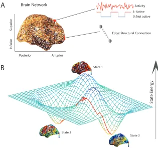
FIGURE 2 : Conceptual Schematic. (A) A weighted structural brain
net-work represents the number of white matter streamlines connecting
brain regions. (B) We model each brain region as a binary object,
being either active or inactive. (C) Using a maximum entropy
model, we infer the full landscape of predicted activity patterns –
binary vectors indicating the regions that are active and the
re-gions that are not active – as well as the energy of each pattern (or
state). We use this mathematical framework to identify and study
local minima in the energy landscape: states predicted to form the
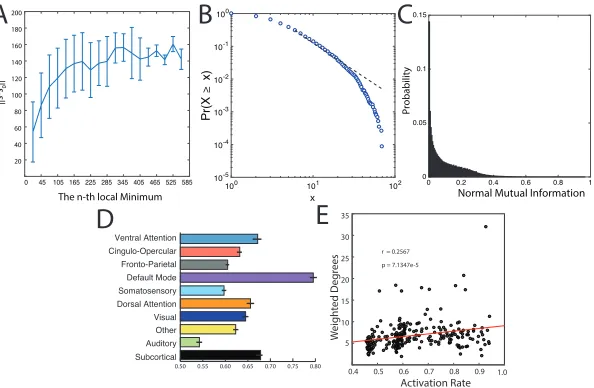
FIGURE 3 : Simulated Activation Rates.(A) The distribution of distances
from the first local minimum to other local minima. Each point
and error-bar is calculated across a bin of 30 minima; error bars
indicate standard error of the mean over the 30 minima. (B) The
probability distribution of the radius of each local minimum is
well-fit by a power-law. The radius of a local minimum is defined as its
distance to the closest sampled point on the energy landscape. (C)
The distribution of the pairwise normalized mutual information
between all pairs of local minima. (D) Average activation rates
for all 14 a priori defined cognitive systems [Power et al. (2011)].
Error bars indicate standard error of the mean across subjects. . 26
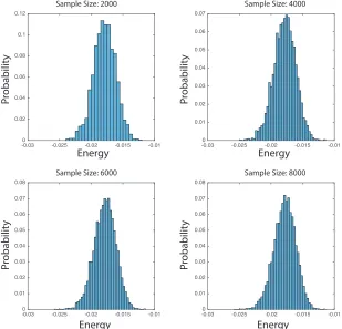
FIGURE 4 : Stability of Energy Distribution with respect to the
Num-ber of Sample Size. We plot the heuristic probability
distribu-tion of the energy for the first 2000, 4000, 6000 and 8000 samples.
We can observe that the shapes are pretty consistent and further
KS-test results ensure the stability. . . 30
FIGURE 5 : Relation between the Regional Energy and the Activation
Rate. Regional Energy and Activation Rate are positively
corre-lated. Here we want to justify that the activation rate is neither
dominated by regional energy nor the weighted degrees. . . 31
FIGURE 6 : Distribution of Between- and Within- System Energy
Tu-ples. We show that the between- and within- system energy
pro-vides C) a better separation for different neural systems compared
to te degrees A), especially B,D) for the Default Mode network,
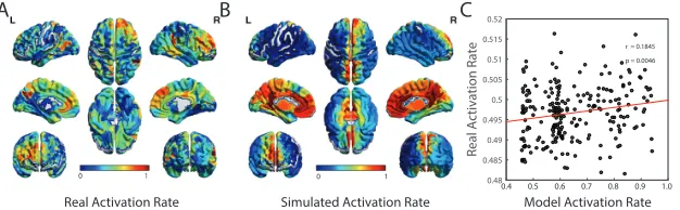
FIGURE 7 : Validating Predicted Activation Rates in Functional
Neu-roimaging Data. (A) From resting state BOLD data acquired
in an independent cohort, we estimated the true activation rate by
transforming the continuous BOLD magnitudes to binary state
vec-tors by thresholding the signals at 0 (see Methods). We use these
binary state vectors to estimate the activation rates of each brain
region across the full resting state scan. Here we show the mean
activation rate of each brain region, averaged over subjects. (B)
For comparison, we also show the mean predicted activation rate
estimated from the local minima of the maximum entropy model,
as defined in Equation [2.4], and averaged over subjects. (C) We
observe that the activation rates estimated from resting state fMRI
data are significantly positively correlated with the activation rates
estimated from the local minima of the maximum entropy model
(Pearson’s correlation coefficientr = 0.18,p= 0.0046). Each data
point represents a brain region, with either observed or predicted
FIGURE 8 : Utilization Energies of Cognitive Systems. (A) Average
within-system energy of each cognitive system; error bars indicate
standard error of the mean across subjects. (B) Average
between-system energy of each cognitive between-system; error bars indicate
stan-dard error of the mean across subjects. (C) The 2-dimensional
plane mapped out by the within- and between-system energies of
different brain systems. Each data point represents a different brain
region, and visual clusters of regions are highlighted with lightly
colored sectors. The sector direction is determined by minimizing
the squared loss in point density of the local cloud and the width
is determined by the orthogonal standard derivation at the center
along the sector direction. In this panel, all data points represent
values averaged across subjects. (D) The percentages of minima
displaying preferential activation of each system; each minima was
assigned to the system which whom it shared the largest normalized
mutual information. Errorbars indicate the differences between the
observed percentages and those of the null distribution with
ran-dom activation patterns across regions. . . 37
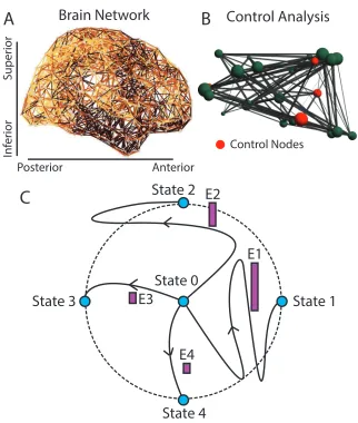
FIGURE 9 : Conceptual Schematic. From weighted brain networks (A), we
estimate control points(B) whose large-scale regional activity can
move the brain into new trajectories that traverse diverse cognitive
functions(C). In panel(C), we show the original state of the system
(state 0), as well as 4 possible states (indicated by the blue circles)
that are equidistant from state 0 in the state space (indicated by
the black circular line), and which can be reached by trajectories
that are more or less energetically costly (indicated by the height
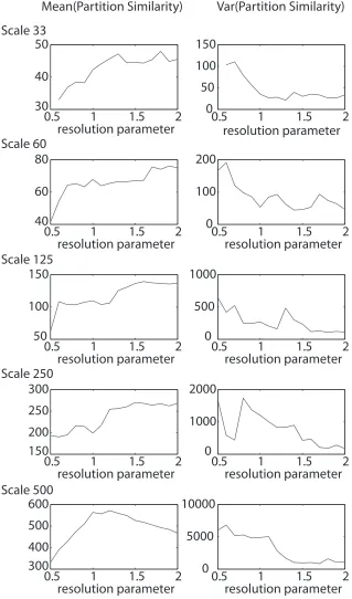
FIGURE 10 : Partition Similarity As a Function of the Resolution
Pa-rameterMean(left)and variance(right)of the partition similarity
estimated using thez-score of the Rand coefficient as a function of
the structural resolution parameterγ, varies from 0.5 to 2 in
incre-ments of 0.1, for the 5 spatial scales of the Lausanne atlas [Hagmann
et al. (2008a)](rows). . . 54
FIGURE 11 : Effect of Boundary Point Criteria ThresholdColor indicates
Pearson correlation coefficient,r, between the vectors of boundary
controllability values estimated for pairs of ρ values in the range
FIGURE 12 : Brain Network Control Properties(A)Average controllability
quantifies control to many easily reached states. Here we show
con-trollability values, averaged across persons, and ranked for all brain
regions plotted on a surface visualization. Warmer colors indicate
larger values of average controllability. (B)Scatter plot of weighted
degree (ranked for all brain regions) versus average
controllabil-ity (Pearson correlation r = 0.91, p = 8 ×10−92). (C) Modal
controllability quantifies control to difficult-to-reach states. Here
we show modal controllability values ranked for all brain regions
plotted on a surface visualization. (D) Scatter plot of weighted
degree (ranked for all brain regions) versus modal controllability
(r =−0.99, p = 2×10−213). (E) Boundary controllability
quan-tifies control to decouple or integrate network modules. Here we
show boundary controllability values ranked for all brain regions
plotted on a surface visualization. (F)Scatter plot of weighted
de-gree (ranked for all brain regions) versus boundary controllability
(r = 0.13, p = 0.03). In panels (A), (C), and (E), warmer
col-ors indicate larger controllability values, which have been averaged
over both replicates and subjects. These results are reliable over a
range of atlas resolutions, and are consistent with findings using a
network composed of only cortical circuitry. Note nodes are sorted
in ascending order of the weighted degree. . . 62
FIGURE 13 : Average Controllability Across Spatial Scales Surface
visu-alizations of the ranked average controllability (AC) values over the
5 spatial scales of the Lausanne atlas [Hagmann et al. (2008a)]. . 63
FIGURE 14 : Modal Controllability Across Spatial Scales Surface
visual-izations of the ranked modal controllability (MC) values over the
FIGURE 15 : Boundary Controllability Across Spatial ScalesSurface
visu-alizations of the ranked boundary controllability (BC) values over
the 5 spatial scales of the Lausanne atlas [Hagmann et al. (2008a)]. 65
FIGURE 16 : Reliability and Conservation of Brain Network Control
Properties Brain network control properties are reliable across
imaging acquisition and conserved in non-human primates. Scatter
plots of weighted degree (ranked for all brain regions) versus(A,D)
average controllability (Pearson correlation coefficient r = 0.88,
p= 1.0×10−78;r = 0.90,p= 4.9×10⁻³⁴),(B,E) modal
controlla-bility (r=−0.99,p= 3.9×10−179;r=−0.99,p= 1.3×10−72), and
(C,F) boundary controllability (r = 0.14, p = 0.028; r = −0.19,
p = 0.074) for (A,B,C) human diffusion tensor imaging data and
FIGURE 17 : Control Roles of Cognitive SystemsCognitive control hubs are
differentially located across cognitive systems. (A)Hubs of average
controllability are preferentially located in the default mode
sys-tem. (B) Hubs of modal controllability are predominantly located
in cognitive control systems, including both the fronto-parietal and
cingulo-opercular systems. (C) Hubs of boundary controllability
are distributed throughout all systems, with the two predominant
systems being ventral and dorsal attention systems. Control hubs
have been identified at the group level as the 30 regions with the
highest controllability values (averaged over replicates and
sub-jects). Raw percentages of control hubs present in each system
have been normalized by the number of regions in the cognitive
system. By applying this normalization, systems composed of a
larger number of regions have the same chance of housing one of
the top 30 control hubs as systems composed of a smaller number
of regions. . . 73
FIGURE 18 : Differential Recruitment of Cognitive Systems to Network
ControlAverage controllability (AC), modal controllability (MC),
and boundary controllability (BC) hubs are differentially located in
default mode (A), fronto-parietal and cingulo-opercular cognitive
control(B), and attentional control(C) systems. Values are
aver-aged over the 3 replicates for each individual; error bars indicate
FIGURE 19 : Control Roles of Cognitive Systems. Cognitive control hubs
are differentially located across cognitive systems. (Left) Hubs
of average controllability are preferentially located in the default
mode system. (Middle) Hubs of modal controllability are
pre-dominantly located in cognitive control systems, including both
the fronto-parietal and cingulo-opercular systems. (Right) Hubs
of boundary controllability are distributed throughout all systems,
with the two predominant systems being ventral and dorsal
atten-tion systems. These anatomical distribuatten-tions are consistent across
different definitions of control hubs as either (Top) the 25 nodes
with the highest control values, (Middle) the top 30 nodes with
the highest control values, or(Bottom)the 35 nodes with the
high-est control values. . . 79
FIGURE 20 : Differential Recruitment of Cognitive Systems to Network
Control. Average controllability (AC), modal controllability (MC),
and boundary controllability (BC) hubs are differentially located in
default mode (A), fronto-parietal and cingulo-opercular cognitive
control (B), and attentional control (C) systems. These results
are consistently observed whether we define control hubs as the
25 nodes with the highest control values(Top Row), the 30 nodes
with the highest control values(Middle Row), or the 35 nodes with
the highest control values(Bottom Row). Values are averaged over
the 3 replicates for each individual; error bars indicate standard
FIGURE 21 : Differential Recruitment of Cognitive Systems to Network
ControlAverage controllability (AC), modal controllability (MC),
and boundary controllability (BC) hubs are differentially located in
default mode (A), fronto-parietal and cingulo-opercular cognitive
control(B), and attentional control(C) systems. Values are
aver-aged over the 3 replicates for each individual; error bars indicate
standard deviation of the mean over subjects. . . 83
FIGURE 22 : Numeric Stability of Trajectories In this figure, we compute
on the average connectivity matrix of th subjects and show(A)The
trajectory’s maximal distance to the target state decreases as the
number of control nodes increases. (B) The trajectory’s maximal
distance to the target state decreases as the balance parameter ρ
increases and becomes “stable” whenρ >0.01. . . 106
FIGURE 23 : Conceptual Schematic. (A)Diffusion imaging data can be used
to infer connectivity from one voxel to any other voxel via diffusion
tractography algorithms. (B) From the tractography, we construct
a weighted network in whichN = 234 brain regions are connected
by the quantitative anisotropy along the tracts linking them (see
Methods). (C) We study the optimal control problem in which
the brain starts from an initial state (red) at timet= 0 and uses
multi-point control (control of multiple regions; blue) to arrive at
FIGURE 24 : Optimal Control Trajectories. (A) We study 3 distinct types
of state transitions in which the initial state is characterized by
high activity in the default mode system, and the target states are
characterized by high activity in auditory (blue), visual (green),
or motor (red) systems. (B) The activation profiles of all N =
234 brain regions as a function of time along the optimal control
trajectory, illustrating that activity magnitudes vary by region and
by time. (C) The average distance from the current state x(t) to
the target statex(T) as a function of time for the trajectories from
default mode system to the auditory, visual, and motor systems,
illustrating behavior in the large state space. (D) The average
control energy utilized by the control set as a function of time for
the trajectories from default mode system to the auditory, visual,
and motor systems. See Fig. S2B for additional information on the
range of these control energy values along the trajectories. Colors
representing target states are identical in panels(A),(C), and (D). 115
FIGURE 25 : Structurally-Driven Task Preference for Control Regions.
(A) Left Regions with high control efficiency (see Eqn 4.20) across
all 3 state transitions: from the default mode to auditory, visual,
and motor systems. Right Scatterplot of the control efficiency with
the average network communicability to the target regions. (B–D)
Regions with high control efficiency for the transition from default
mode to (B) motor, (C) visual, and (D) auditory targets (top);
scatter plot of control efficiency versus normalized network
FIGURE 26 : Robustness of Control in Health and Following Injury. (A)
Theoretically, the brain is fully controllable when every region is a
control point, but may not be fully controllable when fewer regions
are used to effect control. (B)The regions with the highest values of
energetic impact on control trajectories upon removal from the
net-work, on average across subjects and tasks, were the supramarginal
gyrus and the inferior parietal lobule. In general, the healthy group
and the mTBI group displayed similar anatomical patterns of
ener-getic impact. (C) Magnitude and standard derivation of energetic
impact averaged over regions and tasks; boxplots indicate variation
over subjects. After removing outliers in the distribution, patients
wtih mTBI displayed significantly lower values of average
magni-tude of energetic impact (permutation test: p = 2.5×10⁻⁴) and
lower values of the average standard deviation of energetic impact
CHAPTER 1 : Introduction
1.1. What is a brain network?
The word network dates back to the famous Latin phrase opus reticulatum, a brickwork
spreading the diamond-shape bricks over the wall or ground [Briggs (2004)]. Analogous
to the network(graph) in graph theory, which started with Leonhard Euler’s paper Seven
Bridges of K¨onigsberg published in 1736, the intersection points of the bricks form nodes of
a graph(network), and the cracks among the bricks become the edges. The network science
has expanded dramatically with the social media [Ellison et al. (2007)] and the brain imaging
techniques [Lauterbur et al. (1973); Le Bihan et al. (1986); Thulborn et al. (1982)]. Along
with the development in understanding the physics and topological properties of the complex
systems since the mid 1990’s [Albert and Barab´asi (2002); Strogatz (2001); Boccaletti et al.
(2006)], network science identifies its role as an interdisciplinary science to characterize and
analyze the structure and function of network, which turns out to be a fundamental form
of the data structure in this big-data era [McAfee et al. (2012)].
The human brain can be viewed as a network. On micro scale, the neuronal elements
con-stitute the complex brain networks, where the neuron cells consist of the nodes and the
nerve fibers consist of the edges. Outside these nerve fibers, there are various kinds of glial
cells with oligodendrocytes, which constitute the myelin sheaths surrounding the axons.
The diffusion MRI [Basser et al. (1994)] tracks the anisotropic property of water
displace-ment in both the fibers and the myelin sheaths [Beaulieu and Allen (1994)], thus making it
possible to unseal the underlined anatomical structure and to construct a structural brain
network, where the node can either be a voxel or a coherent region and the edge is computed
via measuring the anisotropy between voxels or regions. The most widely applied one is
the fractional anisotropy [Koay et al. (2006)]. The more recent diffusion imaging methods
DSI (Diffusion Spectrum Imaging) improves the Diffusion Tensor Imaging by better
et al. (2007)]. These diffusion imaging methods help construct the structural or anatomical
brain networks. On the other hand, with the development of brain imaging techniques of
higher temporal resolution, like functional MRI, EEG, MEG, researchers assemble
func-tional networks with the edges estimated as certain statistical relations between regional
signals [Biswal et al. (1995); Greicius et al. (2003); Stam et al. (2007)].
On the regional scale, the nature of the brain images makes the graph theory an appropriate
approach to view the brain structure [Iturria-Medina et al. (2007, 2008)]. A bundle of
graphical measures has been applied to quantify both the local and global properties of
the brain network. The brain network displays high clustering in connectivity and short
average path length between regions, thus identifies itself as a small-world network [Watts
and Strogatz (1998); Bassett and Bullmore (2006); Bassett et al. (2006)]. Locally the node
centrality measure quantifies the node’s importance in the network. The nodes with high
contributions are recognized as network hubs. It has been consistently shown in different
scales and parcellations that the precuneate and frontal regions play an important role in the
process of global communication [Iturria-Medina et al. (2008)]. Also, it has been shown that
the medial parietal, frontal and insular regions are confirmed to locate at central network
positions [van den Heuvel et al. (2010); Li et al. (2013); van den Heuvel and Sporns (2011)].
Another widely discussed property of the brain network is the module structure. The
module structures have been discovered in both the anatomical network [Hagmann et al.
(2008b); van den Heuvel and Sporns (2011)] and the functional network [Meunier et al.
(2009b); Power et al. (2011)]. Not only do the modules respond to the brain’s segregation
of functions [Meunier et al. (2009b); Power et al. (2011)], but the dynamics of the module
roles has also been discovered to encode human’s high-level cognitive functions [Bassett
et al. (2011b, 2015, 2011b)] and the development of brain systems [Power et al. (2010); Gu
1.2. Why should we use the control theory to view the brain network?
Conceptually, cognitive control is analogous to the mathematical notions of control used
in engineering, where the state of a complex system can be modulated by energetic input.
Networked systems—like the brain—are particularly interesting systems to control because
of the role of the underlying architecture, which predisposes certain components to
spe-cific control actions. In the brain, neuronal ensembles or regions (nodes) are interlinked
by anatomical wires (edges) in a complex architecture that has an impact on neural
func-tion, development, disease and rehabilitation. It is plausible that the brain could regulate
cognitive function by a transient network-level control process akin to those engineered in
technological, social and cyberphysical systems. Yet, an exact understanding of the
rela-tionship between mathematical measures of controllability and notions of cognitive control
from neuroscience remains elusive.
Practically, now that the brain networks have been identified as a small-world network
with module structures, researchers have now turned to quantifying the dynamics of brain
systems. Not only are the control sets in control theory analogous to the brain’s control
systems, but the methodologies and algorithms developed in control theory enable us to
i) analyze the energy cost and efficiency of the brain system with specific constraints,
ii) quantify controllability of the brain modules and the importance of the control sets,
iii) compare the trajectories with respect to different state transitions and control sets.
Thus, the control theory potentially builds a bridge between the anatomical structure of the
brain and its dynamics of the cognitive control and provides the technical tools to analyze
1.3. Mathematical concepts
We can have a better understanding of the brain’s structure and dynamics when we describe
it in mathematical concepts. In this section, we will first summarize the definitions of some
basic graphical metrics and then introduce the setting of network control theory.
1.3.1. Network Measures
Based on the type of edges, a network can be described as a binary and undirected network
or weighted and directed network. Here we summarize some basic metrics in the following
paragraphs. For more inclusive and comprehensive definition and examples, one can refer
Node
Edge
Community
Connetivity Triangle
Degree, k=3
Shortest Path, L = 3
A graph is denoted asG= (V, E), whereV is the set of nodes andE is the set of edges. The
associated adjacent matrixA with Gis defined as A={aij}such that aij = 1 if and only
ifeij is an existing edge inE. The definition for the weighted and directed is similar to the
binary and undirected network but exclude the constraint that aij =aji. The associated
matrixW ={wij}denotes the weight of edges E={eij}.
Degree Degree of nodei is defined as the sum over the connections related to nodei: :
ki = X
j∈V
aij. (1.1)
Weighted degree of i: kw
i =
P
j∈V wij
(Directed) out-degree of nodei: kout
i =
P
j∈V aij.
(Directed) in-degree of nodei: kout
i =
P
j∈V aji.
Shortest path length Shortest path length between nodei and node j is defined as the
length of the shortest path starting from nodeiand ending at node j:
dij = X
auv∈g{i←j}
auv, (1.2)
where g{i←j} is the shortest path(geodesic) between region i and j. The weighted and
directed shortest path length between node i and node j: dW
ij is defined correspondingly
with the weighted and directed geodesics as well as the mapwij →f(wuv) from the weight
to distance.
Characteristic path lengthCharacteristic path length of the network is defined as
aver-age of shortest paths :
L= 1 n
X
i∈V
Li, (1.3)
where Li is the average distance between node i and all other nodes. For the weighted
average distanceLD
i .
Global efficiencyGlobal efficiency of the network is defined as the average of the inversed
path lengths:
E = 1
n
X
i∈V
Ei=
1 n
X
i∈V
P
j∈V,j6=id
−1 ij
n−1 , (1.4)
where Ei is the efficiency of node i. For the weighted and directed version, replace the dij
with the weighted distancedW
ij and the directed distancedDij.
Clustering Coefficient Clustering coefficient of the network is defined as the ratio of
existing triangles to the possible number of triangles :
C= 1
n
X
i∈V
Ci=
1 n
X
i∈V
2ti
ki(ki−1)
, (1.5)
where Ci is the clustering coefficient of node i and ti is the number of triangles around
node i. For the weighted version, CW = 1 n
P
i∈V CiW = n1
P
i∈V
2tW
i
ki(ki−1). For the directed
version,CD = 1 n
P i∈V
tD
i
(kout
i +kiin)(kiout+kini −1)−2
P
j∈Vaijaji.
ModularityModularity of the network if defined as the normalized sum of the modularity
function over the given partition:
Q= 1
2m
X
i,j∈V
(aij−
kikj
2m)δcicj, (1.6)
whereciis the cluster label of regioniand 2m=Pi,j∈V aij. For the weighted version,QW =
1
2mW
P
i,j∈V(wij−
kWi kjW
2mW )δcicj. For the directed version,Q
D = 1
2mD
P
i,j∈V(aij−
kouti kinj
2mW )δcicj.
Closeness CentralityCloseness centrality of nodeiis defined as the inverse of the average
path lengths:
L−i 1= P n−1 i∈V,j6=idij
. (1.7)
Participation CoefficientThe participation coefficient of nodeiis defined as the squared
ratio of inter-modular connections to the full connections:
ci = 1− X
c∈C
ki(m)
k(i)
2
, (1.8)
where theCis the collection of clusters or modules. For the weighted and directed version,
replace the ki withkWi and kiin and kiout.
Small-wolrdnessSmall-worldness of the network is defined as the quotient of the
normal-ized clustering coefficient and the normalnormal-ized characteristic path length:
S = C/Crand L/Lrand
. (1.9)
For the weighted and directed version, replace the clustering coefficientCwithCW andCD
and the characteristic path lengths with LW and LD. For a typical small-world network,
the measure S1.
1.3.2. Controllability Settings
Mathematically speaking, we can study the controllability of a networked system by defining
a network represented by the graph G = (V,E), where V and E are the vertex and edge
sets, respectively. Let aij be the weight associated with the edge (i, j) ∈ E, and define
the weighted adjacency matrix of G as A = [aij], where aij = 0 whenever (i, j) 6∈ E. We
associate a real value (state) with each node, collect the node states into a vector (network
state), and define the map x:N≥0 →Rn to describe the evolution (network dynamics) of
the network state over time. Given the network and node dynamics, we can use network
control theory to quantitatively examine how the network structure constrains the types of
control that nodes can exert.
To define the dynamics of neural processes, we draw on prior models linking structural brain
neural circuits as a collection of nonlinear dynamic processes, these prior studies have
demonstrated that a significant amount of variance in neural dynamics can be predicted
from simplified linear models. Based on this literature, we employ a simplified noise-free
linear discrete-time and time-invariant network model:
x(t+ 1) =Ax(t) +BKuK(t), (1.10)
where x : R≥0 → RN describes the state (i.e., a measure of the electrical charge, oxygen
level, or firing rate) of brain regions over time, andA∈RN×N is a symmetric and weighted
adjacency matrix. In our case, we construct a weighted adjacency matrix whose elements
indicate the number of white matter streamlines connecting two different brain regions –
denoted here asiandj– and we stabilize this matrix by dividing by the mean edge weight.
While the model employed above is a discrete-time system, we find that the controllability
Gramian is statistically similar to that obtained in a continuous-time system. The diagonal
elements of the matrixAsatisfyAii= 0. The input matrixBKidentifies the control points
K in the brain, where K={k1, . . . , km} and
BK=
ek1 · · · ekm
, (1.11)
andei denotes thei-th canonical vector of dimensionN. The inputuK:R≥0→Rmdenotes
the control strategy.To determine the trajectory from an initial statex0 to a target statexT,
we expose the the evolution dynamics with boundary condition and energy optimization as
following:
min
u
Z T
0
(xT −x)T(xT −x) +ρuTu,
s.t. x˙(t) =Ax+Bu,
x(0) =x0,
x(T) =xT,
where T is the control horizon, and ρ ∈ R≥0. To study the ability of a certain brain
region to influence other regions in arbitrary ways we adopt the control theoretic notion of
controllability. Controllability of a dynamical system refers to the possibility of driving the
state of a dynamical system to a specific target state by means of an external control input
. Classic results in control theory ensure that controllability of the network (1.10) from the
set of network nodes K is equivalent to the controllability Gramian WK being invertible,
where
WK=
∞
X
τ=0
AτBKBTKAτ. (1.13)
1.4. Contribution of my works
Despite the existing literatures about the controllability of complex networks [Liu et al.
(2011); Sorrentino et al. (2007); Yuan et al. (2013)] and the cognitive control of brain
systems [Miller (2000); Ochsner and Gross (2005); MacDonald et al. (2000); Ridderinkhof
et al. (2004); Power et al. (2011)], we are the first to propose a systematic framework of
applying the control theory to analyzing the brain networks and to exploring the possibility
of explaining the cognitive control property based on their underlined anatomical structures
[Gu et al. (2015a)]. Further, we develop the scheme via proper considerations of the energy
issues associated with both of the states and trajectories, thus extend the model from
diagonalizing the static networks to quantifying the dynamical properties of multiple state
transitions in the brain. Our works establish a new subfield in the network neuroscience as
CHAPTER 2 : The Landscape of Neurophysiological Activity Implicit in Brain
Network Structure
2.1. Introduction
A human’s adaptability to rapidly changing environments depends critically on the brain’s
ability to carefully control the time within (and transitions among) different states. Here,
we use the term state to refer to a pattern of activity across neurons or brain regions
[Tang et al. (2012)]. The recent era of brain mapping has beautifully demonstrated that
the pattern of activity across the brain or portions thereof [Mahmoudi et al. (2012)] differs
in different cognitive states [Gazzaniga (2013)]. These variable patterns of activity have
enabled the study of cognitive function via the manipulation of distinct task elements
[Gazzaniga (2013)], the combination of task elements [Szameitat et al. (2011); Alavash et al.
(2015)], or the temporal interleaving of task elements [Ruge et al. (2013); Muhle-Karbe
et al. (2014)]. Such methods for studying cognitive function are built on the traditional
view of mental chronectomy [Donders (1969)], which suggests that brain states are additive
and therefore separable in both space and time (although see [Mattar et al. (2015)] for a
discussion of potential caveats).
Philosophically, the supposed separability and additivity of brain states suggests the
pres-ence of strong constraints on the patterns of activations that can be elicited by the human’s
environment. The two most common types of constraints studied in the literature are
energetic constraints and structural constraints [Bullmore and Sporns (2012)]. Energetic
constraints refer to fundamental limits on the evolution [Niven and Laughlin (2008)] or
us-age of neural systems [Attwell and Laughlin (2001)], which inform the costs of establishing
and maintaining functional connections between anatomically distributed neurons [Bassett
et al. (2010)]. Such constraints can be collectively studied within the broad theory of brain
function posited by the free energy principal – a notion drawn from statistical physics and
energy in neural activity [Friston et al. (2006); Friston (2010)]. The posited preference for
low energy states motivates an examination of the time within and transitions among local
minimums of a predicted energy landscape of brain activity [Moreno-Bote et al. (2007);
Tsodyks et al. (1998)].
While energetic costs likely form critical constraints on functional brain dynamics, an
ar-guably equally important influence is the underlying structure and anatomy linking brain
areas. Intuitively, quickly changing the activity of two brain regions that are not directly
connected to one another by a structural pathway may be more challenging than changing
the activity of two regions that are directly connected [Achard and Bullmore (2007);
Bas-sett et al. (2010)]. Indeed, the role of structural connectivity in constraining and shaping
brain dynamics has been the topic of intense neuroscientific inquiry in recent years [Honey
et al. (2009, 2010); Deco and Jirsa (2012); Go˜ni et al. (2014); Becker et al. (2016)]. Evidence
suggests that the pattern of connections between brain regions directly informs not only the
ease with which the brain may control state transitions [Gu et al. (2015a)], but also the ease
with which one can externally elicit a state transition using non-invasive neurostimulation
[Muldoon et al. (2016b)].
While energy and anatomy both form critical constraints on brain dynamics, they have
largely been studied in isolation, hampering an understanding of their collective influence.
Here, we propose a novel framework that combines energetic and structural constraints on
brain state dynamics in a free energy model explicitly informed by structural connectivity.
Using this framework, we map out the predicted energy landscape of brain states, identify
local minima in the energy landscape, and study the profile of activation patterns present
in these minima. Our approach offers fundamental insights into the distinct role that
brain regions and larger cognitive systems play in distributing energy to enable cognitive
function. Further, the results lay important groundwork for the study of energy landscapes
in psychiatric disease and neurological disorders, where brain state transitions are known to
State 1
State 2
State 3
Brain Network
Anterior Posterior
Inf
er
ior
Super
ior
1: Active 0: Not active
Edge: Structural Connection Activity
Sta
te Ener
gy
A
B
2.2. Models and Materials
2.2.1. Human DSI Data Acquisition and Preprocessing
Diffusion spectrum images (DSI) were acquired for a total of 48 subjects (mean age 22.6±5.1
years, 24 female, 2 left handed) along with aT1 weighted anatomical scan at each scanning
session [Cieslak and Grafton (2014)]. Of these subjects, 41 were scanned ones, 1 was scanned
twice, and 6 were scanned three times, for a total of 61 scans.
DSI scans sampled 257 directions using aQ5 half shell acquisition scheme with a maximum
b value of 5000 and an isotropic voxel size of 2.4mm. We utilized an axial acquisition with
the following parameters: T R= 11.4s, T E= 138ms, 51 slices, FoV (231,231,123 mm). All
participants volunteered with informed written consent in accordance with the Institutional
Review Board/Human Subjects Committee, University of California, Santa Barbara.
DSI data were reconstructed in DSI Studio (www.dsi-studio.labsolver.org) using q-space
diffeomorphic reconstruction (QSDR) [Yeh and Tseng (2011)]. QSDR first reconstructs
diffusion weighted images in native space and computes the quantitative anisotropy (QA)
in each voxel. These QA values are used to warp the brain to a template QA volume
in MNI space using the SPM nonlinear registration algorithm. Once in MNI space, spin
density functions were again reconstructed with a mean diffusion distance of 1.25 mm using
three fiber orientations per voxel. Fiber tracking was performed in DSI Studio with an
angular cutoff of 55◦, step size of 1.0 mm, minimum length of 10 mm, spin density function
smoothing of 0.0, maximum length of 400 mm and a QA threshold determined by DWI signal
in the CSF. Deterministic fiber tracking using a modified FACT algorithm was performed
until 100,000 streamlines were reconstructed for each individual.
2.2.2. Structural Network Construction
Anatomical scans were segmented using FreeSurfer [Dale et al. (1999)] and parcellated
et al. (2008a)]. A parcellation scheme including 234 regions was registered to the B0 volume
from each subject’s DSI data. The B0 to MNI voxel mapping produced via QSDR was used
to map region labels from native space to MNI coordinates. To extend region labels through
the gray/white matter interface, the atlas was dilated by 4mm. Dilation was accomplished
by filling non-labeled voxels with the statistical mode of their neighbors’ labels. In the event
of a tie, one of the modes was arbitrarily selected. Each streamline was labeled according
to its terminal region pair.
From these data, we built structural brain networks from each of the 61 diffusion spectrum
imaging scans. Consistent with previous work [Bassett et al. (2010, 2011a); Hermundstad
et al. (2013, 2014); Klimm et al. (2014); Gu et al. (2015a); Muldoon et al. (2016a,b);
Sizemore et al. (2015)], we defined these structural brain networks from the streamlines
linking N = 234 large-scale cortical and subcortical regions extracted from the Lausanne
atlas [Hagmann et al. (2008a)]. We summarize these estimates in a weighted adjacency
matrixA whose entries Aij reflect the structural connectivity between regioniand region
j (Fig. 2A).
Following [Gu et al. (2015a)], here we use an edge weight definition based on thequantitative
anisotropy (QA). QA is described by Yeh et. al (2010) as a measurement of the signal
strength for a specific fiber population ˆa in an ODF Ψ(ˆa) Yeh et al. (2010); Tuch (2004).
QA is given by the difference between Ψ(ˆa) and the isotropic component of the spin density
function (SDF, ψ) ISO (ψ) scaled by the SDF’s scaling constant. Along-streamline QA
was calculated based on the angles actually used when tracking each streamline. Although
along-streamline QA is more specific to the anatomical structure being tracked, QA is more
sensitive to MRI artifacts such as B1 inhomogeneity. QA is calculated for each streamline.
We then averaged values over all streamlines connecting a pair of regions, and used this
2.2.3. Resting state fMRI data
As an interesting comparison to the computational model, we used resting state fMRI data
collected from an independent cohort composed of 25 healthy right-handed adult subjects
(15 female), with a mean age of 19.6 years (STD 2.06 year). All subjects gave informed
consent in writing, in accordance with the Institutional Review Board of the University
of California, Santa Barbara. Resting-state fMRI scans were collected on a 3.0-T Siemens
Tim Trio scanner equipped with high performance gradients at the University of California,
Santa Barbara Brain Imaging Center. A T2*-weighted echo-planar imaging (EPI) sequence
was used (TR=2000 ms; TE=30 ms; flip angle=90; acquisition matrix=64×64; FOV=192
mm; acquisition voxel size = 3×3×3.5 mm; 37 interleaved slices; acquisition length=410s).
We preprocessed the resting state fMRI data using an in-house script adapted from the
workflows described in detail elsewhere [Baird et al. (2013); Satterthwaite et al. (2013)].
The first four volumes of each sequence were dropped to control for instability effects of the
scanner. Slice timing and motion correction were performed in AFNIusing 3dvolreg and
FreeSurfers BBRegister was used to co-register functional and anatomical spaces. Brain,
CSF, and WM masks were extracted, the time series were masked with the brain mask, and
grand-mean scaling was applied. The temporal derivative of the original 6 displacement
and rotation motion parameters was obtained and the quadratic term was calculated for
each of these 12 motion parameters, resulting in a total of 24 motion parameters which were
regressed from the signal. The principal components of physiological noise were estimated
using CompCor (aCompCor and tCompCor) and these components were additionally
re-gressed from the signal. The global signal was not rere-gressed. Finally, signals were low
passed below 0.1 Hz and high passed above 0.01 Hz in AFNI. To extract regional brain
sig-nals from the voxel-level time series, a mask for each brain region in the Lausanne2008 atlas
was obtained and FreeSurfer was used to individually map regions to the subject space. A
winner-takes-all algorithm was used to combine mapped regions into a single mask. The
Following data preprocessing and time series extraction, we next turned to extracting
ob-served brain states. Importantly, physiological changes relating to neural computations take
place on a time scale much smaller than the time scale of BOLD image acquisition. Thus, we
treat each TR as representing a distinct brain state. To maximize consistency between the
model-based and data-based approaches, we transformed the continuous BOLD magnitude
values into a binary state vector by thresholding regional BOLD signals at 0. From the set
of binary state vectors across all TRs, we defined activation rates in a manner identical to
that described for the maximum entropy model data.
2.2.4. Defining an Energy Landscape.
We begin by defining a brain state both intuitively and in mathematical terms. A brain
state is a macroscopic pattern of BOLD activity acrossKregions of the brain (Fig. 2A). For
simplicity, here we study the case in which each brain regionican be either active (σi= 1)
or inactive (σi = 0). Then, the binary vectorσ = (σ1, σ2, . . . , σK) respresents a brain state
configuration.
Next, we wish to define the energy of a brain state. We build on prior work demonstrating
the neurophysiological relevance of maximum entropy models in estimating the energy of
brain states in rest and task conditions [Watanabe et al. (2013, 2014)]. For a given state
σ, we write its energy in the second order expansion:
E(σ) =−1
2
X
i6=j
Jijσiσj − X
i
Jiσi, (2.1)
where J represents an interaction matrix whose elements Jij indicate the strength of the
interaction between region i and region j. If Jij >0, this edge (i, j) decreases the energy
of state σ, while if Jij < 0, this edge (i, j) increases the energy of state σ. The column
sum of the structural brain network, Ji = Pj|Jij|/ √
K, is the strength of region i. In
the thermodynamic equilibrium of the system associated with the energy defined in Eqn
P(σ)∝e−E(σ).
The choice of the interaction matrix is an important one, particularly as it tunes the relative
contribution of edges to the system energy. In this study, we seek to study structural
interactions in light of an appropriate null model. We therefore define the interaction matrix
to be equal to the modularity matrix [Newman (2006)] of the structural brain network:
Jij =
1
2m(A−pp
T/2m)
ij (2.2)
fori6=j, whereAis the adjacency matrix,pi =PiK=1Aij, and 2m=PKj=1pj. This choice
ensures that any elementJij measures the difference between the strength of the edgeAij in
the brain and the expected strength of that edge in an appropriate null model (here given
as the Newman-Girvan null model [Clauset et al. (2004)]). If the edge is stronger than
expected, it will decrease the energy of the whole system when activated, while if the edge
is weaker than expected, it will increase the energy of the whole system when activated.
2.2.5. Discovering Local Minima.
The model described above provides an explicit correspondence between a brain’s state and
the energy of that state, in essence formalizing a multidimensional landscape on which brain
dynamics may occur. We now turn to identifying and characterizing the local minima of
that energy landscape (Fig. 2C). We begin by defining a local minimum: a binary stateσ∗=
(σ∗
1, . . . , σK∗) is a local minimum ifE(σ)≥E(σ∗) for all vectorsσsatisfying||σ−σ∗||1 = 1,
which means that the stateσ∗realizes the lowest energy among its neighboring states within
the closed unit sphere. We wish to collect all local minima in a matrixΣ∗ with
Σ∗= σ∗
1,1 σ1∗,2 · · · σ1∗,N
σ∗
2,1 σ2∗,2 · · · σ2∗,N
..
. ... . .. ...
σK,∗ 1 σ∗K,2 · · · σ∗K,N
K×N
where N is the number of local minima and K is the number of nodes in the structural
brain network (or equivalently the cardinality of the adjacency matrixA).
Now that we have defined a local minimum of the energy landscape, we wish to discover
these local minima given the pattern of white matter connections represented in structural
brain networks. To discover local minima of E(σ), we first note that the total number of
states σ = (σ1, . . . , σK) is 2K, which – when K = 234 – prohibits an exhaustive analysis
of all possibilities. Moreover, the problem of finding the ground state is an NP-complete
problem [Cipra (2000)], and thus it is unrealistic to expect to identify all local minima of
a structural brain network. We therefore choose to employ a clever heuristic to identify
local minima. Specifically, we combine the Metropolis Sampling method [Metropolis et al.
(1953)] and a steep search algorithm using gradient descent methods. We identify a starting
position by choosing a state uniformly at random from the set of all possible states. Then,
we step through the energy landscape via a random walk driven by the Metropolis Sampling
criteria (see Algorithm 1). At each point on the walk, we use the steep search algorithm to
identify the closest local minimum.
Algorithm 1:Heuristic Algorithm to Sample the Energy Landscape to Identify Local
Minima.
1 Let σj be the vector obtained by changing the value of thej-th entry of σ;
2 for t = 1 : N do
3 Randomly select an indexj∈ {1, ..., K};
4 Set ˜σt=σt=σjt−1 with probabilityp= min(1, e
−β∗(E( ˜σ)−E(σt−1))) and
˜
σt=σt=σt−1 otherwise;
5 whileσ˜t is not a local minimum do
6 Setj∗= arg minjE( ˜σjt);
7 Set ˜σt= ˜σj ∗
t ;
8 Setσ∗t = ˜σt;
and β is the temperature parameter which can be absorbed in E(σ). In the context of
any sampling procedure, it is important to determine the number of samples necessary
to adequately cover the space. Theoretically, we wish to identify a number of samples N
following which the distribution of energies of the local minima remains stable. Practically
speaking, we choose 4 million samples in this study, and demonstrate the stability of the
energy distribution in the Supplement. A second important consideration is to determine
the initial state, that is the state from which the random walk begins. Here we choose this
state uniformly at random from the set of all possible states. However, this dependence on a
uniform probability distribution may not be consistent with the actual probability of states
in the energy landscape. We therefore must ensure that our results are not dependent on
our choice of initial state. To ensure independence from the initial state, we dismiss the first
30,000 local minima identified, and we demonstrate in the Supplement that this procedure
ensures our results are not dependent on the choice of initial state.
2.2.6. Characterizing Local Minima.
Following collection of local minima, we wished to characterize their nature as well as their
relationships to one another. First, we estimated the radius of each local minimum as the
Hamming distance from the minimum to the closest sampled point on energy landscape.
Next, calculated the Hamming distance from each local minimum to the first sampled local
minimum, a second quantification of the diversity of the energy lanscape that we traverse in
our sampling. Finally, we quantify how diverse the observed local minima are by calculating
the pairwise normalized mutual information [Manning et al. (2008)] of each pair of local
minima.
Next, we wished to understand the role of different regions and cognitive systems in the
minimal energy states. Cognitive systems are sets of brain regions that show coordinated
activity profiles in resting state or task-based BOLD fMRI data [Mattar et al. (2015)]. They
include the visual, somatosensory, motor, auditory, default mode, salience, fronto-parietal,
the specific association of regions of interest to cognitive systems are exactly as listed in
[Gu et al. (2015a)] and based originally on results described in [Power et al. (2011)]. We
characterize the roles of these systems in the local minima by assessing their activation
rates, as well as the utilization energies required for communication within and between
systems.
2.2.7. Activation Rates
Intuitively, we define the activation rate of a node ias the average activation state of that
node over all the local minima. Formally, the activation rate for region iis defined as
ri=
PN
l=1σil∗
N , (2.4)
where l indexes over states, and recall N is the number of local minima. The computed
activation rate offers a prediction of which regions are more versus less active across the
local minima (that is, the brain’s locally “stable ” states), and can be directly compared
with the resting state activation rate estimated from empirical fMRI data.
2.2.8. Utilization Energies
To complement the information provided by the activation rates, we also defined the
en-ergetic costs associated with utilizing within- and between-systems interactions. We note
that each cognitive system is a subnetwork of the whole brain network. We use the index
set I to indicate the set of nodes associated with the cognitive system, and thus |I| gives
the number of nodes in the system. Then, for a given state σ, the within-system energy
measures the cost associated with the set of interactions constituting the subnetwork. The
between-system energy measures the cost associated with the set of interactions between
EW(σ) = − 1
2|I|(|I| −1)
X
i6=j,i,j∈I
Jijσiσj
EB(σ) = − 1
2|I|(K− |I|)
X
i∈I,j /∈I
Jijσiσj
where EW measures the within-system energy, EB measures the between-system energy,
and the normalization coefficients 1/(|I||I| −1|), 1/(|I|(K− |I|)) are chosen by considering
the number of the corresponding interactions.
2.2.9. Permutation Tests for State Association
For a given local minimum configuration σ∗, we associate it with systemiσ∗,
iσ∗= arg max
i NMI(σ
∗,σsys
i ),
whereσsysi is the configuration pattern of systemisuch that the corresponding regions for
systemiare activated and the others not and where “NMI” refers to the Normalized Mutual
Information [Manning et al. (2008)], which is used to measure the similarities between the
two states. To obtain the null distribution, for each local minimum configuration σ∗ in
the collectionΣ∗, we permute the configuration at each position ofσ∗ to achieve a random
configuration with the same activation rate, and we then compute the associated percentage
in each system. Then we repeat this procedure to generate N samples and construct the
null distribution of the probability of being configured as each system pattern. Considering
the large size of the state collection, the variance of the samples in the null distribution will
2.2.10. Predicted Functional Connectivity
The approach outlined above offers an assessment of activity states expected in the brain
given the pattern of underlying structural connectivity and the expectation that the brain
seeks to minimize energy expenditure. In addition to these direct outputs, the approach
also offers a means to predict expected functional connectivity. For two regions i and j,
their predicted functional connectivity is defined as the similarity between their activation
patterns through theN local minima. Letσj = (σj,1, σj,2, . . . , σj,N) andk(·,·) :σ×σ→R
be a pre-defined similarity function (here we use a Pearson correlation). The predicted
functional connectivity matrixC= (cij)K×K is then defined ascij =k(σi,σj). In the body
of the results section of this manuscript, we assess the relationship between the functional
connectivity predicted by the model, and the functional connectivity observed in resting
state fMRI data collected from an independent cohort.
2.3. Results
2.3.1. Local Minima in the Brain’s Energy Landscape
By sampling the energy landscape of each structural connectivity matrix, we identified
an average of approximately 450 local minima or low energy brain states: binary vectors
indicating the pattern of active and inactive brain regions (see Methods). On average across
the 61 scans, 144 brain regions were active in a given local minimum, representing 61.70%
of the total (standard deviation: 6.04%). This large percentage suggests that the brain
may utilize a broad set of rich and diverse activations to perform cognitive functions [Cha
(2016)], rather than activation patterns localized to small geographic areas.
To quantify this diversity, we examined the location of minima on the energy landscape, the
size of the basins surrounding the minima, and the mutual information between minima.
First, we estimated the distance from the first local minima identified to all subsequent
minima (see Methods; Fig. 3A). We observe an order of magnitude change in the distance