A New Multi-Class WSVM Classification to Imbalanced Human Activity Dataset

A New Multi-Class WSVM Classification to

Imbalanced Human Activity Dataset

M’hamed B. Abidine and Belkacem Fergani Speech Communication & Signal Processing Laboratory

Faculty of Electronics and Computer Sciences, USTHB, Algiers, Algeria [email protected], [email protected]

Abstract—This paper is concerned with the class imbalance

problem in activity recognition field which has been known to hinder the learning performance of classification algorithms. To deal this problem, we propose a new version of the multi-class Weighted Support Vector Machines (WSVM) method to perform automatic recognition of activities in a smart home environment. Then, we compare this approach with CRF, k-NN and SVM considered as the reference methods. Our experimental results carried out on various real world imbalanced datasets show that the new WSVM is capable of solving the class imbalance problem by improving the class accuracy of activity classification compared to other methods.

Index Terms—Imbalanced data, support vectors machines,

activity recognition, machine learning.

I. INTRODUCTION

In recent years, the classification problem with imbalanced data has received considerable attention in areas such as Machine Learning and Pattern Recognition. A two-class data set is said to be imbalanced (or skewed) when one of the classes (the minority class) is heavily under-represented in comparison to the other class (the majority one) in training dataset. In this paper, we are concerned with the problem of imbalanced classification activity recognition field to assist sick or elderly people for performing daily life activities [1] such as eating, brushing teeth, dressing, using the toilet, using the telephone, bathing and so on. In this situation, it is costly to misclassify examples from the minority class, the learning system may have difficulties to learn the concept related to the minority class, and therefore, results in a classifier’s suboptimal performance.

Activity recognition datasets are generally imbalanced, meaning certain activities occur more frequently than others. These differences in frequency may corresponds to how often a particular activity is performed (e.g. sleeping is generally done once a day, while toileting is done several times a day), or to the number of timeslices an activity takes up (e.g. a sleeping activity generally takes up considerably more timeslices than a toileting activity). However, not incorporating this class imbalance

results in an evaluation that may lead to disastrous consequences for elderly person.

In recent years, there have been several attempts at dealing with the class imbalance problem [2, 3]. Traditionally, research on this topic has mainly focused on a number of solutions both at the data and algorithmic levels.

At the data level, these solutions include many different forms of re-sampling such as oversampling [4] (in which new samples are created for the minority class), undersampling [5] (where, the samples are eliminated for the majority class) and combination of the above techniques. At the algorithmic level, the solutions include adjusting the costs associated with misclassification so as to improve performance [6], adjusting the probabilistic estimate at the tree leaf (when working with decision trees), adjusting the decision threshold, and recognition-based (i.e., learning from one class [7]) rather than discrimination-based (two class) learning.

Many popular machine learning algorithms have been tried to see how well they can cope with the imbalanced situation, e.g. k-nearest neighbors (k-NN) [8], Support Vector Machine (SVM) [9, 10], random forests [11], but none of them has found to be superior over one another. Our objective is to deal the class imbalance problem to perform automatic recognition of activities from binary sensor patterns in a smart home. The main contribution of our work is twofold. Firstly, we propose a new version of the discriminative method named Weighted Support Vector Machines (WSVM) in order to avoid the overfitting caused by imbalanced class samples. Secondly, this method is compared with Conditional Random Fields (CRF), k-NN and the traditional SVM utilized as reference methods.

The next section II describes the k-NN, SVM baseline methods and the new WSVM method. Then, the results and evaluation are presented in section III. Lastly, we will conclude with some future work.

II. DISCRIMINATIVE METHODS FOR ACTIVITY RECOGNITION

A. Conditional Random Fields (CRF)

CRF has a single exponential model for the conditional probability (1) of the entire sequence of labels Y given an input observation sequence X. CRF is defined by a Manuscript received August 25, 2013; revised September 25, 2013;

weighted sum of K feature functionsf_ithat will return a 0 or 1 depending on the values of the input variables and therefore determines whether a potential should be included in the calculation. Each feature function carries a weight λ_i that gives its strength for the proposed label. These weights are the parameters we want to find when learning the model. CRF Model parameters can be learned using an iterative gradient method by maximizing the conditional probability distribution defined as

= ∑ ∑ = = −

⎟

⎠

⎞

⎜

⎝

⎛

T

t i t t t

K

i if y y x X

Z X Y P

1 1 ( , 1, )

exp ) ( 1 ) |

( λ (1)

With ∑ ∑ ⎟

⎠ ⎞ ⎜ ⎝ ⎛ ∑ =

_⎟

⎠

⎞

⎜

⎝

⎛

= = − y T

t i t t t

K

i if y y x X

Z

1 1 ( , 1, )

exp )

( λ (2)

One of the main consequences of this choice is that while learning the parameters of a CRF we avoid modelling the distribution of the observations, p(x). As a result, we can only use CRF to perform inference (and not to generate data), which is a characteristic of the discriminative models. In ADL recognition, the only thing we are interested in is classification and therefore CRF fit our purpose perfectly.

To find the predicted label y for new observed features, we take the maximum of the conditional probability.

yˆ(x)=argmax_y p(y|x) (3)

B. k-Nearest Neighbors (k-NN)

The k-nearest neighbors algorithm is amongst the simplest of all machine learning algorithms [8], and therefore easy to implement. The m training instances

n R

x∈ are vectors in an n-dimensional feature space, each with a class label. In the k-NN method, the result of a new query is classified based on the majority of the k -NN category. The classifiers do not use any model for fitting and are only based on memory to store the feature vectors and class labels. They work based on the minimum distance from an unlabelled vector (a test point) to the training instances to determine the k-NN. The k positive integer is a user-defined constant. Usually Euclidean distance is used as the distance metric.

C. Support Vector Machines (SVM)

Support Vector Machines (SVM) based on statistical learning theory were initially proposed by Vapnik [9]. SVM classifies data by determining a set of support vectors, which are members of the set of training inputs that outline a hyperplane into a higher dimensional space (feature space).

For a two class problem, we assume that we have a training set

{

(

x_i,y_i

)

}

_im₌₁ where x_i∈Rn are the observations and yi are class labels either 1 or -1. The

primal SVM formulation maximizes margin 2/K(w,w) between two classes and minimizes the training error ξi

simultaneously by solving the following optimization problem : m i b x w y to subject C w w K i i i T i m i i b w , ,... 1 , 0 , 1 ) ) ( ( ) , ( . 2 / 1 min 1 , , = ≥ − ≥ + ∑ + = ξ ξ φ ξ ξ (4)

where w is normal to the hyperplane, b is the translation factor of the hyperplane to the origin andφ(.) is a non-linear function which maps the input space into a feature space defined by K(x_i,x_j)=φ(x_i)Tφ(x_j). That is, the dot product in that feature space is equivalent to a kernel function K(.,.) of the input space. In a support vector

machines, we need to select a kernel function K(.,.) and

the regularization parameter C.

The radial basis kernel function (RBF) is easy to implement; its computation is not as complex as the other kernel’s. So we choose the RBF kernel:

⎟

⎠

⎞

⎜

⎝

⎛

− ₋

= ₂ 2

2 1 exp ) ,

(x y x_i x_j K

σ where σ is the width

parameter. The construction of such functions is described by the Mercer conditions [12]. The regularization parameter C is used to control the trade-off between maximization of the margin width and minimizing the number of training error of nonseparable samples in the training set represented by slack variables ξi in order to avoid the problem of overfitting [8].

In practice the parameters σ and C are varied through a wide range of values and the optimal performance assessed using a separate validation set or a technique known as cross-validation for verifying performance using only training set.

The dual formulation of the soft margin SVM can be reformulated as [9]:

( , )

2 1

max im1 i mi 1 mj 1 i jyiyjK xi xj

i

∑ ∑ −

∑=α = =αα

α (5)

Subject to ∑im=1α_iyi =0 and 0≤αi ≤C,

where α_i >0 are Lagrange multipliers. The training samples for which Lagrangian multipliers are not zero are called support vectors.

Solving (5) forα gives a decision function in the original space for classifying a test point x∈Rn[9]

⎟

⎠

⎞

⎜

⎝

⎛

_{∑ +} = = sv m

i iyiK x xi b x

f

1 ( , )

sgn )

( α (6)

with m_svis the number of support vectors x_i∈Rn.

In this study, a software package LibSVM [13] was used to implement the multiclass classifier algorithm. It uses the one-versus-one method [9]. In this work, we focus on the new WSVM discriminative method to appropriately tackle the problem of class imbalance. D. Weighted SVM (WSVM)

undesirable. An extension of the SVM, weighted SVM (WSVM), was presented to cope with this problem. Two different penalty constraints were introduced for the minority and majority classes:

m i b x w y to subject C C w w K i i i T i y i y i b

w _{i i}

, ,... 1 , 0 , 1 ) ) ( ( ) , ( . 2 / 1 min 1 1 , , = ≥ − ≥ + ∑ + ∑ + − = − = + ξ ξ φ ξ ξ ξ (7)

The WSVM dual formulation gives the same Lagrangian as in the original SVM in (5), but with different constraints on α_ias follows:

0≤α_i ≤C₊, if y_i =+1, and (8) 0≤α_i ≤C₋, if y_i =−1

+

C and C− are regularization parameters for positive and negative classes, respectively, to construct a classifier for multiple classes. They are used to control the trade-off between margin and training error. Some authors [14, 15] have proposed adjusting different penalty parameters to different class which effectively improves the low classification accuracy caused by imbalanced samples. For example, it is highly possible to achieve the high classification accuracy by simply classifying all samples as the class with majority samples (positive class), therefore the minority class (negative class) is the error training. Veropoulos et al. in [14] propose to increase the tradeoff associated with the minority class.

E. New Weighted SVM

The new Weighted SVM method advocates analytic parameter selection of the C+ and C− regularization parameters with a new criterion directly from the training data, on the basis of the proportion of class data. This criterion respects this reasoning that is to say that the tradeoff C−associated with the smallest class is largein order to improve the low classification accuracy caused by imbalanced samples. It allows the user to set individual weights for individual training examples, which are then used in WSVM training. We give the main regularization value Ci in function of m+ the number of

majority classes samples and mi the number of other classes samples, it is given by:

C_i =

[

m₊/m_i

]

(9)

[ ] is integer function andC_i∈

{

1,...,m+/m_i

}

, i =1,...,N For the two-class training problem, the primal optimization problem of the new WSVM can be constructed via this criterion and become:

m i ξ ξ b x φ w y ξ m m ξ w w K i i i T i y i y i ξ b,

w, _{i i}

, 1,... 0, , 1 ) ) ( ( to subject ] [ ) , ( 1/2 min 1

1

/

.

= ≥ − ≥ + ∑ + ∑ + − = − + = (10)

The new WSVM dual formulation gives the same Lagrangian as in the WSVM in (5) with C₊ =1 and

− + − =m m

C

/

.

III. EXPERIMENTAL RESULTS AND DISCUSSION

A. Datasets

For the experiments, we use an openly accessible datasets gathered from three houses having different layouts and different number of sensors [16], see Table 1. Each sensor is attached to a wireless sensor network node. Data are collected using binary sensors such as reed switches to determine open-close states of doors and cupboards; pressure mats to identify sitting on a couch or lying in bed; mercury contacts to detect the movements of objects like drawers; passive infrared sensors to detect motion in a specific area; float sensors to measure the toilet being flushed. Time slices for which no annotation is available are collected in a separate activity labelled “Idle”. The data were collected by a Base-Station and labelled using a Wireless Bluetooth headset or a handwritten diary.

TABLE I.

DETAILS OF THEDATASETS RECORDED IN THREE DIFFERENT HOUSES USING WIRELESS SENSOR NETWORKS

Houses House A House B House C

Age 26 28 57

Annotation Bluetooth headset Bluetooth headset handwritten diary

Setting Apartment Apartment House

Rooms 3 2 6

Duration 25days 13days 18days

Sensors 14 22 21

TABLE II.

LIST OF ACTIVITIES FOR EACH HOUSE AND THE NUMBER OF OBSERVATIONS

House A House B House C

Idle(6031) Leaving(16856) Toileting(382) Showering(264) Brush teeth(39)

Sleeping(11592) Breakfast(93)

Dinner(330) Snack(47) Drink(53)

Idle(5598) Leaving(10835)

Toileting(75) Showering(112) Brush teeth(41) Sleeping(6057)

Dressing(46) Prep.Breakfast(81) Prep.Dinner(90)

Drink(12) Dishes(34) Eat Dinner(54) Eat Breakfast(143)

Play piano(492)

Idle(2732) Leaving(11993)

Eating(376) Toileting(243) Showering(191) Brush teeth(102) Shaving(67) Sleeping(7738) Dressing(112) Medication(16)

Breakfast(73) Lunch(62) Dinner(291)

Snack(24) Drink(34) Relax(2435)

B. Setup and Performance Measures

repeated l times, with different training sets of size (l - 1) and report the average performance measure.

Sensors outputs are binary and represented in a feature space which is used by the model to recognize the activities performed. We do not use the raw sensor data representation as observations, instead we use the “Change point” and “Last” representation which have been shown to give much better results in activity recognition [17]. The raw sensor representation simply gives a 1 when the sensor is firing and a 0 otherwise. The “change point” representation gives a 1 when the sensor reading changes from 0 to 1 or from 1 to 0 and gives a 0 otherwise. While the last sensor representation continues to assign a 1 to the last sensor that changed state until a new sensor changes state. (See Figure 1)

Figure 1. Example of sensor firing showing the a) Raw, b) Change point and c) Last observation representation. [17]

As the activity instances were imbalanced between classes, we evaluate the performance of our models by two measures, the accuracy and the class accuracy. The accuracy shows the percentage of correctly classified instances, the class accuracy shows the average percentage of correctly classified instances per classes. These measures are defined as follows:

m

i true i erred

Accuracy ₌ ∑mi=1[inf ()= ()] ₍₁₁₎

[

]

∑ ∑ =

=

= =

⎥⎦

⎤

⎢⎣

⎡

N

c c

m

i c c

m

i true i erred N

Class c

1

1 inf () ()

1 ₍₁₂₎

in which [a = b] is a binary indicator giving 1 when true and 0 when false. m is the total number of samples, N is the number of classes and mc the total number of

samples for class c.

A problem with the accuracy measure is that it does not take differences in the frequency of activities into account. Therefore, the class accuracy should be the primary way to evaluate an activity classifier’s performance. C. Results

We compared the performance of the CRF, k-NN, SVM (using cross validation research) and the proposed WSVM method on the imbalanced dataset of the houses (A), (B) and (C) in which majority class are all classes that have a longer duration (e.g. ’Idle’, ’Leaving’ and ’Sleeping’ for the house (A) and house (B); ’Idle’, ’Leaving’, ’Sleeping’ and ’Relax’ for the house (C)), while others are the minority classes. These algorithms are tested under MATLAB environment and the SVM algorithm is tested with implementation LibSVM [13].

In our experiments, the SVM hyper-parameters(σ, C) have been optimized in the range (0.1-2) and (0.1-10000) respectively to maximize the class accuracy of

leave-one-day-out cross validation technique. The best pair parameters (σopt, Copt) = (1, 5), (σopt, Copt) = (1, 5) and (σopt,

Copt) = (2, 500) are used for the three datasets (A), (B) and

(C) respectively, see Tables III, IV, V. The k parameter for the k-NN method is optimised by the leave-one-day-out cross validation technique. Then, we tried to find the penalty parameters Cadaptatif (class) adapted for different

classes by using our proposed criterion, see Tables VI, VII, VIII.

TABLE III.

SELECTION OF PARAMETER COPT WITH THE CROSS VALIDATION FOR C-SVM FOR THE HOUSE (A)

Copt 0.1 5 50 500 1000 5000 10000

Class (%) 51.7 61 61 61 61 61 61

TABLE IV.

SELECTION OF PARAMETER COPT WITH THE CROSS VALIDATION FOR THE

HOUSE (B)

Copt 0.1 5 50 500 1000 5000 10000

Class (%) 40.6 50.3 50.2 50.2 50.2 50.2 50.2

TABLE V.

SELECTION OF PARAMETER COPT WITH THE CROSS VALIDATION FOR THE

HOUSE (C)

Copt 0.1 5 50 500 1000 5000 10000

Class (%) 25.5 35.2 35.5 35.6 35.6 35.6 35.6

Our empirical results in tables III, IV, V suggest that the value of regularization parameter C has negligible effect on the generalization performance (as long as C is larger than a certain threshold analytically determined from the training data (C =5 for the houses (A) and (B); C =500 for the house (C)).

TABLE VI.

SELECTION OF PARAMETER COPT ADAPTED FOR EACH CLASS WITH OUR

CRITERION FOR THE NEW WSVM FOR HOUSE (A)

ADL Id Le To Sh Bt Sl Br Di Sn Dr

Copt 2 1 43 63 432 1 181 51 358 306

TABLE VII.

SELECTION OF PARAMETER COPT ADAPTED FOR EACH CLASS WITH OUR

CRITERION FOR THE NEW WSVM FOR HOUSE (B)

ADL Id Le To Sh B.t Sl Dr P.b P.d Dr Copt 1 1 144 96 264 1 235 133 120 902

Di E.d E.br P.p

318 200 75 22

TABLE VIII.

SELECTION OF PARAMETER COPT ADAPTED FOR EACH CLASS WITH OUR

CRITERION FOR THE NEW WSVM FOR HOUSE (C)

ADL Id Le Ea To Sh B.t Sh Sl Dr

Copt 4 1 31 49 62 117 179 1 107

Me Br Lu Di Sn Dr Re

749 164 193 41 499 352 4

TABLE IX.

ACCURACY AND CLASS ACCURACY FOR CRF,K-NN,SVM AND THE NEW WSVM FOR THE THREE HOUSES

Houses Models Accuracy Class

A CRF [16]

k-NNk=7

SVM

WSVM+our criterion

91% 90.5%

92.1%

88%

57% 55.9% 50.3%

62.0%

B CRF [16]

k-NN k=9

SVM

WSVM+our criterion

92%

67.7% 85.5% 62.7%

46% 31.3% 39.3%

46.4%

C CRF[16]

k-NN k=1

SVM

WSVM+our criterion

78% 78.4%

80.7%

76.8%

30% 35.7% 35.6%

37.2%

Table IX shown the summary of the accuracy and the class accuracy obtained with the concatenation of Changepoint and Last representations for CRF, k-NN, SVM and the new WSVM using our criterion for all datasets. This table shows that the proposed WSVM performs better in terms of class accuracy, while SVM performs better for the houses (A), (C) in terms of accuracy.

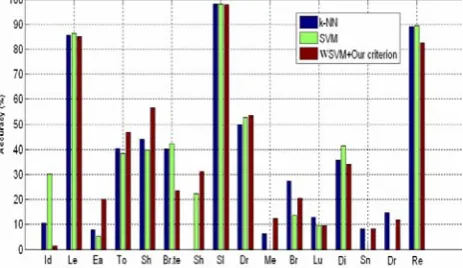
In order to find out which activities are relatively harder to be recognized, we report in figures 2, 3, 4 the classification results in terms of accuracy measure for each activity with k-NN, SVM and the proposed WSVM methods for different houses.

In Figure 2, the activities ’Idle’, ’Leaving’ and ’Sleeping’ give the highest accuracy for SVM method. The table shows that the proposed WSVM mainly performs better for the minority activities : ’Showering’, ’Brush teeth’, ’Breakfast’, ’Dinner’, ’Snack’ and ’Drink’. Most

confusion takes place in the ’Brush teeth’ activity.

Figure 2. Comparison of accuracy of classification measure for each activity between k-NN, SVM and the new WSVM with house (A).

In Figure 3, for the proposed WSVM, the minority

activities ’Toileting’, ’Brush teeth’, ’Dressing’, ’Prep.Breakfast’, ’Prep.Dinner’, ’Dishe

s’, ’Eat Dinner’ and ’Eat Breakfast’, give the highest accuracy while the ’Showering’ and ’Play piano’ activities are less accurate compared to SVM. It can be

seen that the ’Drink’ activity with 12 instances has not been recognized.

Figure 3. Comparison of accuracy of classification measure for each activity between k-NN, SVM and the new WSVM with house (B).

Finally, We can see in Figure 4 that with the proposal

WSVM, the minority activities ’Eating’, ’Showering’, ’Toileting’, ’Shaving’, ’

Dressing’, ’Medication’ and ’Snack’ are better recognized comparatively with others methods. It can be seen that most of the confusion obtained with the new WSVM takes place in ’Idle’ activity.

Figure 4. Comparison of accuracy of classification measure for each activity between k-NN, SVM and the new WSVM with house (C).

Our results give us early experimental evidence that our proposed method combined WSVM with our proposed criterion works better for model classification; it consistently outperforms the other methods in terms of the class accuracy for all datasets. k-NN and SVM perform better for the majority activities. This explains the high accuracy of k-NN and SVM methods .

D. Discussion

regularization parameter C for all class. When not considering the weights in SVM formulation, this affect the classifiers performances and favorites the classification of majority activities (’Idle’, ’Leaving’, ’Sleeping’ and ’Relax’). In other words, k-NN and SVM overfit for these activities since they occur more often in the datasets.

The new WSVM considering the weights in SVM formulation and including the individual setting of parameter C for each class separately shows that WSVM becomes more robust for classifying the minority activities compared to the others classification methods. It is observed for the new WSVM, the ’Idle’ activity gave the worst results compared to the others methods. In particular, this activity often takes up a large amount of time slices but is usually not a very important activity to recognize. It might therefore be useful to less weigh this activity.

IV. CONCLUSION

In this paper, we have proposed a new version of multi-class WSVM learning method that has the power to effectively control the performance generalization by dealing imbalanced datasets in human activity recognition field in smart homes. We showed that WSVM based our proposed criterion is effective to classify multiclass sensory data over common techniques such as CRF, k-NN and SVM using an equal misclassification cost. The WSVM using different penalty parameters for each activity improves the low classification accuracy caused by imbalanced datasets.

REFERENCES

[1] N. Zouba, F. Bremond, M. Thonnat, A. Anfosso, E. Pascual, P. Mallea, V. Mailland, and O. Guerin. “A computer system to monitor older adults at home : Preliminary results,” Gerontechnology Journal, 8(3) :129– 139, July 2009.

[2] N. Chawla. Data mining for imbalanced datasets: An overview. Data Mining and Knowledge Discovery Handbook. pp. 875-886, 2010.

[3] N. V. Chawla, N. Japkowicz, and A. Kotcz, “Editorial: special issue on learning from imbalanced data sets,” SIGKDD Explorations, vol. 6, no. 1, pp. 1–6, 2004. doi: 10.1145/1007730.1007733

[4] N. Chawla, K. Bowyer, L. Hall, and P. Kegelmeyer, “SMOTE: Synthetic Minority Over-sampling Technique,” Journal of Artificial Intelligence Research, 16, 321-357, 2002. doi: 10.1613/jair.953

[5] X. Chen, B. Gerlach, and D. Casasent, “Pruning support vectors for imbalanced data classification,” In Proc. of IJCNN, 1883-88, 2005. doi: 10.1109/IJCNN.2005.1556167

[6] P. Domingos, “MetaCost: a general method for making classifiers cost-sensitive,” Proc. of the Fifth ACM SIGKDD, pp. 155-164, 1999. doi: 10.1145/312129.312220

[7] A. Raskutti. and A. Kowalczyk, “Extreme rebalancing for svms: a svm study,” SIGKDD Explorations, 6(1), 60-69, 2004. doi: 10.1145/1007730.1007739

[8] C. Bishop, “Pattern Recognition and Machine Learning, Springer,” New York, ISBN: 978-0-387-31073-2, 2006.

[9] V.N. Vapnik, “Statistical Learning Theory,” New York: John Wiley & Sons, ISBN: 978-0-471-03003-4, 1998.

[10] M.B. Abidine and B. Fergani, “Evaluating C-SVM, CRF and LDA classification for daily activity recognition,” in Proc. of IEEE ICMCS, Tangier-Morocco, May 2012, pp. 272 -277. doi: 10.1109/ICMCS.2012.6320300

[11] C. Chen, A. Liaw, and L. Breiman, “Using random forest to learn imbalanced data,” Technical Report Technical report 666, Statistics Department, University of California, 2004.

[12] J. Shawe-Taylor and N. Cristianini, “Kernel Methods for Pattern Analysis”, Cambridge University Press, p220, 2004.

[13] C. C. Chang and C. J. Lin, LIBSVM: [Online]. Available: http://www.csie.ntu.edu.tw/~cjlin-/libsvm/.

[14] K. Veropoulos, C. Campbell and N. Cristianini, “Controlling the sensitivity of support vector machines,” Proceedings of the International Joint Conference on AI, 1999, pp. 55-60.

[15] N. Thai-Nghe, “Cost-Sensitive Learning Methods for Imbalanced Data,” Intl. Joint Conf. on Neural Networks, 2010. doi: 10.1109/IJCNN.2010.5596486

[16] T.L.M. van Kasteren, H. Alemdar and C. Ersoy, “Effective Performance Metrics for Evaluating Activity Recognition Methods,” ARCS 2011 Workshop on Context-Systems Design, Evaluation and Optimisation, Italy, 2011.

[17] T. van Kasteren, A. Noulas, G. Englebienne, and B. Krose, “Accurate activity recognition in a home setting,” in UbiComp ’08. New York, NY, USA: ACM, 2008, pp. 1-9. doi: 10.1145/1409635.1409637

M’hamed B. Abidine was born in

Algiers, Algeria, in 1985.Hereceived the B.S degree in Exact Sciences, Algiers, Algeria in 2002. Then the M.S and the Magister degrees from the Faculty of Electronics and Computer Sciences, University of Sciences and Technology Houari Boumediene (USTHB), Algiers, Algeria, in 2007 and 2010, respectively. Currently, he is an Assistant Professor, Researcher and he prepared the PH.D at the Faculty of Electronics and Computer Sciences, USTHB, Algiers, Algeria.

His research focuses on Pattern Recognition and Machine Learning methods, and Activity Recognition using wireless sensor networks and systems RFID.

Belkacem Fergani was born in Medea