Bayesian Network Based Threat Assessment Method for Vehicle

Bayesian Network Based Threat Assessment

Method for Vehicle

Ming Cen

School of Automation, Chongqing University of Posts and Telecommunications, Chongqing, P. R. China Email: [email protected]

Yanan Guo, Kun Lu

School of Automation, Chongqing University of Posts and Telecommunications, Chongqing, P. R. China Email: [email protected], [email protected]

Abstract—An exact threat level assessment method is necessary to improve safety of vehicles, but the traffic environment is not taken into account adequately in existing approaches. This paper presents a Bayesian network based method to improve the effect of vehicles threat evaluation. In the method, various factors threatening vehicle safety are analyzed, and a Bayesian network model with environmental factors and vehicle factors is introduced to describe the threat level of vehicles. The local conditional probability tables of the method are given also. Then threat index of vehicles integrating multiple factors can be obtained by Message-passing algorithm. Experimental results show that the method can reflect the threat level of vehicles accurately, and calculational costs meet the requirement of real-time application.

Index Terms—Vehicle threat assessment; Bayesian network; threat assessment model; environmental factors

I. INTRODUCTION

With the increase of vehicles, traffic accident has become one of the world-wide serious problems of modern society, and how to avoid accident has been a significant research topic. However, using the passive safety technologies to significantly decrease the probability of traffic accident is very difficult. Collision warning system can avoid collisions by 37% -74% according to forecasts, so the vehicle anti-collision warning system is the necessary trend of vehicle safety technology [1].

Vehicle threat level assessment method is one of the key technologies for vehicle anti-collision warning system. In order to determine and act correctly to avoid collision, the threat level of the target must be assessed accurately. Currently there are some anti-collision methods of vehicles. The collision threat index can be obtained by calculating the front and rear braking distance [2]. The warning distance and the braking distance of vehicle can be calculated with the acceleration of host and target vehicle, and be compared with measured headway to evaluate the threat index. Using Kaman circle [3] method and Monte Carlo method [4, 5], relative velocity and azimuth data of the obstacles in front of vehicle are acquired to estimate the poses of vehicle

and the object, and then the probability of collision can be calculated to give corresponding warning to the driver. A vehicle active safety framework that performs trajectory planning, threat assessment and hazard avoidance in a unified manner is described [6]. Although anti-collision warning is achieved to some degree by different models, these approaches are insufficient because the influences of environmental factors are ignored.

On the other hand, a series of threat assessment theories are applied in the military field widely. For example, support vector machine method is used for target threat assessment in air combat [7]. By the method, the air combat capability and air combat situation of the target are selected as the indexes to rank the threat assessment, where air combat situation indices include the angle, distance and relative velocity index and air combat capability indices include the maneuverability, firepower, etc. Then the threat level of air combat target can be estimated accurately using support vector machines model. A Bayesian network based hostile target threat level assessment method introduces the menace type, ability to counter and weapon employment zone as input parameters of Bayesian network to calculate the threat level of menace target [8, 9]. The intuitionistic fuzzy decision based solution formulates the battlefield situation assessment as a comprehensive evaluation problem [10]. Then intuitionistic fuzzy based comprehensive evaluation model and the index system for battlefield situation assessment are established, and approaches to effectiveness measures for evaluating goals and normalization of their values are described. A new method integrating Delphi method and analytic hierarchy process to find weight vectors of goals are discussed also. But few of those methods are applied in threat assessment of vehicles.

To improve the effect of vehicles threat evaluation, a Bayesian network method for threat level assessment is presented. In the method, environmental factors and vehicle factors are integrated in a Bayesian network model to describe the threat level of vehicles. Experimental results show the effectiveness of the method.

A typical architecture of vehicle anti-collision warning system is showed in Figure 1, it includes three parts: perception, analysis and decision, and action and perform.

Figure 1. architecture of vehicle anti-collision warning system

In perception, environment, vehicle and driver information are obtained by on-board sensors. In analysis and decision, the data from perception are integrated in a model to evaluate the situation and threat of the vehicle. In action and perform, the warning or necessary control action are implemented according to the result of assessment [11].

In the aspect of vehicle threat assessment, the existing solutions of vehicle threat assessment mainly consider the influence of the distance and velocity. For example, the distance and velocity between vehicles are obtained by sensors, and the collision threat index is determined by calculating the front and rear braking distance [2]. The threat index Iw can be expressed as





2

max max

2 2

f rel f

w f

v v v

d v

a a

  _ _ 

 _  _

 

(1)

2 max

1 2

br rel

d _v _ a  ₍₂₎

br w

w br

d d I

d d  

 (3) balance of reobjective fac Where d is the actual distance, dbr is maximum braking

distance, dw is the warning distance, vf is the target

vehicle velocity, vrsl is relative velocity, is the

maximum deceleration, and τ is reaction time of the driver. Apparently the threat index is related to distance, velocity and braking distance. The threat index from Eq.(1) - (3) is exact for dry pavement scenario, but it is unreliable for execrable environment with low visibility or slippery road because of warning and braking distances increased rapidly. Apparently the environment factors could influence the threat index.

max a

In the Monte Carlo method, measuring the kinematics parameters of target and estimating the target trajectory, if it intersectes with the trajectory of host vehicle, it is determined that collision will occur. Then the collision probability can be obtained by calculating the ratio of collisions times and numbersof sampling particles [4, 5]. Although the simpleness of Monte Carlo method and the capability of calculating multiple scenarios and unknown quantities, considering that the accuracy of the algorithm is related to sampling numbers, there is a contradiction

between the accuracy and real-time performance. The more the sampling numbers, the more exact the algoritm, but the more the calculating costs.

Therefore, a comprehensive model integrating various influence element is necessary to improve the threat assessment method, and real-time requirement of the algorithm is vital also. As an effective tool of knowledge representation and reasoning, Bayesian network is with strong capability of multi-source information fusion and expression [12], and widely used in threat assessment [13], situation awareness [14] and other fields. Bayesian network based threat assessment method can correctly describe the causality between threat elements and threat level , and obtain an integrated assessment result of the threat level. So this approach can provide an effective solution for vehicle threat assessment.

Ⅲ. BAYESIAN NETWORK MODEL FOR VEHICLE THREAT ASSESSMENT

A. Bayesian network model of vehicle threat assessment

Before assessing threat level of vehicle by Bayesian network, threat factors influencing driving safety and their interrelationship should be analyzed, and modeled with a Bayesian network.

There are many factors affecting driving safety, and can be separated into subjective factors and objective factors mainly. Subjective factors refer to the driver's ological state (overtaking psychology, frustration ology, emotional and combative psychology, etc.), tive factors mainly refer to driving environment such as road condition, velocity, vehicles density and vehicles distance, etc. Objective factors can be obtained

te, laser, infrared, radar and other sensors, but there is no effective approach for accurate extraction and measurement of subjective factors. In order to keep the al time and accuracy requirement, only the tors which are most closely associated with the driving safety are selected to establish vehicle threat assessment model.

psych h objec psyc

by satelli

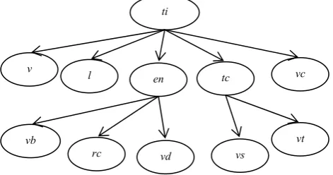
Figure 2. Bayesian network model of vehicle threat assessment

The model is shown in Figure 2 where threat index is divided into high (HT), medium (MT), low (LT) three levels. Let the influence factors set of threat level be Xb,

Xb = { v, l, en, tc, vc}

Where v is the relative velocity and l is the distance of target and the vehicle, en is the parameter representing

vc v

vt ti

l _{en tc}

vb

rc _vd vs

Action and Perform

Warning

Control intervention

Analysis and Decision

Safety decision

Risk analysis Environment

detection

Perception

Vehicle sensing

the influence of environmental factors, tc is the threat capabilities of the target, and vc is condition of host vehicle. The higher the relative velocity, the shorter the distance, the worse the environment, the greater the target threat capabilities, and the worse the vehicle condition, then the higher threat level to host vehicle.

The relative velocity and distance of target and the vehicle can be obtained by vehicle-borne radar. The relative velocity is divided into high speed (HS), normal speed (NS) and low speed (LS), and the distance is divided into risk distance (RD), moderate distance (MD) and security distance (SD). The host vehicle condition can be assessed from the warnings provided by the on-board dashon-board, such as tire pressure, brake block, oil pressure, water temperature and so on. The condition is good (GVC) if no fault warning occurs, and is moderate (MVC) when there is one warning, and is bad (BVC) in case of more than one warning.

Let the influence factors set of threat capabilities of the target vehicle be Xc,

Xc = { vt, vs}

Where vt is target vehicle type and vs is kinematics status. The target type is divided into large vehicle(LV), middle-sized vehicle(MV) and small vehicle (SV), and the vehicle state is divided into passive acceleration (PA), zero acceleration (ZA), and negative acceleration (NA). The target vehicle type and kinematics status can be obtained by image sensors and vehicle-borne radar. According to the direction of target vehicle acceleration, if the acceleration exceeds the threshold, the status of target vehicle could be considered as positive or negative acceleratio, else as zero acceleration. When accelerating, the larger the vehicle type, the higher threat level to host vehicle. Threat vehicle type can be obtained by image sensor, the acceleration and deceleration state can be obtained by vehicle-borne radar.

Similarly, the worse the environmental conditions, the greater the threat level to host vehicle. Let the environmental factors set is Xd

Xd = {vb, rc, vd}

Where vb is visibility, rc is road condition and vd is vehicle density. Visibility vb is divided into far visibility (FV), normal visibility (NV) and near visibility (NV), road condition rc is divided into dry road condition (DR), wet road condition (WR) and ice road condition (IR), and vehicles density is divided into high density (HD), normal density (ND) and low density (LD). The information of visibility can be provided by a visibility meter [15], and road condition can be obtained by road condition identification technology [16, 17]. Vehicle density is related to the velocity of host vehicle. When velocity increases, the critical distance and detection range of threat target increase correspondingly.

For any node xi of the model, it is presumed that when

parent node set Xf of xi is given, xi and all

non-descendant nodes of xi are conditional independent, and

any subset of Xf does not meet this condition. Moreover,

each node in the model has a local conditional probability table (LCPT) to quantitatively describes the effect of the immediate predece

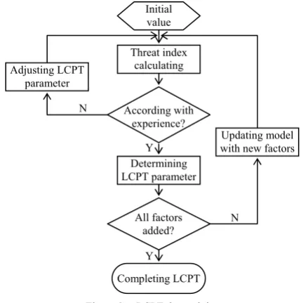
B. Determination of LCPT

After establishing the Bayesian network model of vehicle threat assessment, we need to determine LCPT of each node. There are two main approaches to obtain LCPT, one is using the knowledge of domain expert, the other is through lots of tests and parameters learning [18]. Because of inevitable subjectivity and inaccuracy of experts knowledge base, and imperfection of expert knowledge base for vehicle threat assessment currently, the second approach is adopted.

Step 1 Initial value setting.

The first step of determining LCPT is to set LCPT initial values and design a group of scenarioes to start up the algorithm.

Step 2 Threat index assessing.

Selecting single threat factor as variant and fixing others to obtain a simplified model, the threat index is calculated to assess the effect of the threat factor.

Step 3 Comparing and correcting.

Comparing the threat index from Step 2 and experimental data in [2] or expert experience, and adjusting corresponding LCPT again and again, the appropriate LCPT can be obtained.

Updating the threat model by adding residual threat factors successively, and repeating step 2 to 3, the complete LCPT can be obtained.

ssors [1].

Figure 3. LCPT determining

For instance, the LCPT determination process of relative velocity, distance and environment is shown as follows. Presuming relative velocity and vehicle distance as the main factors of threat index, when the relative velocity is high and the distance is short, no matter how the other threat factors change the threat index is high, but it would tend to zero when the relative velocity reduce and the distance increase. For the scenario of high relative velocity and short distance, let the conditional probability of high threat level is 0.7 and low is 0.1. Considering the influence of relative velocity and distance only, the threat index is 0.83. Comparing with [2] and expert experience, the error is 8.79% approximately. In view of that the threat level of high relative velocity is

Y Y Threat index

calculating

Determining LCPT parameter

Initial value

Adjusting LCPT parameter

Updating model with new factors N

N According with

experience?

All factors added?

higher than that of short distance, increasing the conditional probability of high relative velocity and decreasing the one of low relative velocity appropriately, a more proper threat index is obtained. Adjusting, calculating and comparing repeatedly, the conditional probability of the relative velocity and the distance according with experimental data and expert experience is determined.

Updating the threat model by adding environmental factor, for adverse circumstances, the influnce of environment increases gradually along with increasing relative velocity and decreasing vehicle distance. Because the threat index is 0.91 and close to the alarm threshold when high relative velocity and short vehicle distance, the effect of environmental factor in this scenario can be reduced, and that in moderate relative velocity and distance can be increased approximately. According to expert experiences and actual situation, it is reasonable that the threat index increase by 20% for moderate relative velocity and distance and increase by 10% for high relative velocity and short distance in adverse circumstances. The other influence factors can be added to the threat model similarily to obtain complete LCPT with high reliability. It is given as follows.

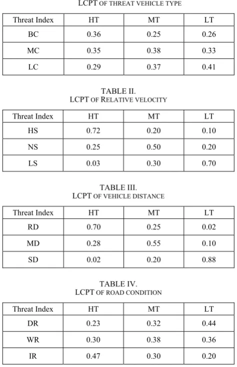
TABLE I.

LCPT OF THREAT VEHICLE TYPE

Threat Index HT MT LT

BC 0.36 0.25 0.26

MC 0.35 0.38 0.33

LC 0.29 0.37 0.41

TABLE II. LCPT OF RELATIVE VELOCITY

Threat Index HT MT LT

HS 0.72 0.20 0.10

NS 0.25 0.50 0.20

LS 0.03 0.30 0.70

TABLE III. LCPT OF VEHICLE DISTANCE

Threat Index HT MT LT

RD 0.70 0.25 0.02

MD 0.28 0.55 0.10

SD 0.02 0.20 0.88

TABLE IV. LCPT OF ROAD CONDITION

Threat Index HT MT LT

DR 0.23 0.32 0.44

WR 0.30 0.38 0.36

IR 0.47 0.30 0.20

Ⅳ. REASONING PROCESS OF THE THREAT ASSESSMENT MODEL

After determing of the threat assessment model and corresponding LCPT, a suitable reasoning algorithm according with the model characteristic is required to update the network to obtain the threat index.

Typically, the reasoning algorithms of Bayesian network include message-passing algorithm [19], junction tree algorithm [20], bucket elimination algorithm [21], etc. Considering that the vehicle threat model is a single connected network, and the path is short generally, the message-passing algorithm is suitable for the threat model reasoning to meet the real time requirement [22]. In the algorithm, each node calculates own posterior probability according to the message from evidence nodes and internal conditional probability of the node, and propagates to adjacent nodes, until influence of the evidence spreads to all nodes of the network.

The essential of the Bayesian network based threat assessment method for vehicle is calculating the posterior probability distribution p(x|E) of the threat index node ti

according to vehicle and environment parameter evidence set E={e1, e2, …, en}.

Let Xf and Xs are parent and child notes set of any note

xi in figure 2 respectively, Xf = {xf1, xf2, … , xfn}, Xs

={xs1, xs2, … , xsm}. eX

 _{denotes the message transmitted}

to xi though child notes set Xs, and X is the message

transmitted to x

e

i though parent notes set Xf.

The reasoning steps of threat assessment model are given as follows:

Step 1 node initialization.

Let π(xi) and λ(xi) is the message transmitted from the

parent notes subset Xf and the child notes subset Xs, and

si is the status of node xi. Initializing the threat evidence

nodes, it is satisfied that

(4)

( ) 1 ( ) 1

i

i i

x

if s e x

 

 

  

 _

 i

i

 

and

(5)

( ) 0 ( ) 0

i

i i

x

if s e x

 

 

  

 _



For all non-evidence nodes xi, λ(xi)=1 if xi has no child

note, and π(xi) = p(si) if xi has no parent note.

Step 2 posterior probability updating.

If note xi receives the message from the parent notes

set Xf, π(xi) is

 





1

1

, 1

| , ,

f fn

n i f fn fi

x x i

x p x x x x

 









 

(6)

If note xi receives the message from the child notes set

Xs, λ(xi) is

 

 

m i

j si

x x

 







Then the message from note xi to parent notes xfi is

 





 

xi fj i fj i i

x P x x x

and the message from note xi to child notes xsj is

 

 

 

xi sj i sk

k j

x x x

  







Where is normalization constant. Then posterior probability distribution of note x





,

X X

p e e  _   

  

i



i under the

threat evidence set E is obtained as







 



   

p x E p x e p e x  x x (10)

Repeating the step 2, until influence of the evidence spreads to all nodes of the network, the posterior

probability of the node ti is the threat index.

.

Ⅴ SIMULATION RESULTS

A. Contrast simulation

To evaluate the effect of the method presented, same scenarios in [2] is used and simulation results of the two methods are compared. In scenario 1, the relative velocity of target vehicle and host vehicle is high and distance is far. In Scenario 2, the relative velocity is high and distance is moderate. In Scenario 3, the relative velocity of target vehicle and host vehicle is high, and distance is short. The environmental factors are ignored in the scenarios. The comparison of simulation results is shown in Table V.

TABLE V.

COMPARISON OF THREAT INDEX WITHOUT ENVIRONMENTAL FACTORS

Threat Index Method Presented References 2

Scenario 1 0.10 0.13

Scenario 2 0.63 0.63

Scenario 3 0.91 0.92

Comparing two groups of simulation results, it can be concluded that the threat index from Bayesian network method is consistent with the one from [2], and the threat index from method presented is accurate.

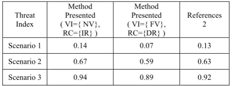
Environmental factors is taken into account in the method presented. To comparing the influnce of environmental factors, two senarios with better and worse environment are adopted. Calculating threat index of two senarios by method presented, the simulation results are shown in Table VI.

TABLE VI.

COMPARISON OF THREAT INDEX INCLUDE ENVIRONMENTAL FACTORS

Threat Index

Method Presented ( VI={ NV},

RC={IR} )

Method Presented ( VI={ FV}, RC={DR} )

References 2

Scenario 1 0.14 0.07 0.13

Scenario 2 0.67 0.59 0.63

Scenario 3 0.94 0.89 0.92

It is shown that the threat index of the vehicle in worse environment is lager than that in better environment.

t the result coincides with the fact, and the expression of the environmental factors in method presented is appropriate.

Apparen

B. Synthetic scenario simulation

Considering the following scenario include a host vehicle and three target vehicles. The host vehicle is in

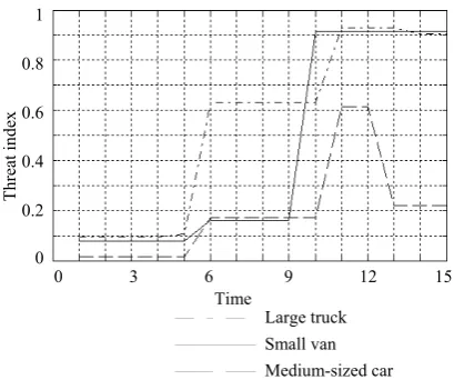
vehicle condition. Target vehicle No.1 is a large truck and approaches host vehicle from far to near quickly, and road condition varied from bad to good. Target vehicle No.2 is a medium-sized car with moderate velocity and approaches host vehicle from far to near, and along with the approach of the vehicles, the road condition becomes bad and the target vehicle begins to slow down. Target vehicle No.3 is a small van approaching host vehicle from far to near, but the velocity of the van is from slow to fast. Along with the approach of the vehicles, the velocity of the van is high and road conditions is bad. Applying Message-passing algorithm and Bucket Elimination algorithm as reasoning method to calculate threat index of the host vehicle respectively, the simulation results are shown in Figure 4 and Figure 5.

good

The effect of target vehicle type and environmental factors can be seen from Figure 4 and Figure 5. From time 1 to 5, when the distance, velocity and scenario keep invariant, it is obvious that the greater the target vehicle, the higher the threat index. From time 6 to 10, the threat index increased along with vehicle distance decreasing gradually. From time 11 to 15, the threat level of the medium-sized car approaching with low speed decreases significantly, and the threat level of truck in poor road condition is higher than that in good road condition.

Figure 4. Message-passing algorithm 1

0.8

0.6

0.4

0.2

0

0 3 6 9 12 15 Time

Th

reat

in

de

x

Figure 5. Bucket Elimination algorithm

A. Calculating performance

To evaluate the calculating performance of the method presented, the Message-passing algorithm and Bucket Elimination algorithm are executed 100 times in PC and ARM9 processor respectively, and the result is shown in Figure 6 and Figure 7.

Figure 6. Comparison of calculating performance of two reasoning algorithm in PC

In Bucket Elimination algorithm, reliability of only one node can be calculated each time, and the problem of finding the optimal elimination order is not resolved properly, so calculating efficiency of the algorithm is restricted. Because the Bayesian network model presented is a third-order model with 10 nodes, the calculating efficiency of the two algorithms are almost the same. The average time consuming of Bucket elimination algorithm is 0.011s in PC and 0.077s in ARM9, and that of Message-passing algorithm is 0.010s in PC and 0.075s in ARM9. The results also show that the method presented can meet the real time reqirement of vehicle threat assessment.

Figure 7. Comparison of calculating performance of two reasoning algorithm in ARM9

Ⅵ. CONCLUSIONS

According to the characteristics of the vehicle threat, an approach to vehicle threat assessment based on Bayesian network is presented. The threat factors influencing traffic safety, including environment factors, are analyzed to establish the model, and the effectiveness of the method is verified by simulation. Bayesian network algorithm is with strong mathematical basis, multi-source information fusion capability and many other advantages, so it suits the requirement of vehicle threat assessment. Furthermore, mutiple factors is considered in the model, so the method presented can provide more accurate vehicle threat level.

ACKNOWLEDGMENT

This work is supported by Science and Technology Project of Chongqing Municipal Education Commission under the Grant No. KJ110521 and Natural Science Foundation Project of Chongqing under the Grant No. CSTC 2009BB2281.

REFERENCES

[1] Han Chongzhao, Zhu Hongyan, Duan Zhansheng, “Multi-source information fusion,” Beijing: Tsinghua University Press, 2006

[2] Hsin-Han Chiang, Bing-Fei Wu, Tsu-Tian Lee, “Integrated headway adaptation with collision avoidance system for intelligent vehicles,” in Conf. Proc. IEEE Int. Conf. Syst. Man Cybern. 2007, pp. 3276-3281

[3] Nico Kaempchen, Bruno Schiele, Klaus Dietmayer, “Situation assessment of an autonomous emergency brake for arbitrary vehicle-to-vehicle collision scenarios,” IEEE Transactions on Intelligent Transportation Systems, vol. 10, pp. 678-687, 2009

[4] C. Mertz, “A 2D collision warning framework based on a monte carlo approach,” in Proceedings of ITS America's 14th Annual Meeting and Exposition, 2004.

[5] Eidehall Andreas, Petersson Lars, “Threat assessment for general road scenes using Monte Carlo sampling,” in IEEE Conf Intell Transport Syst Proc ITSC, pp. 1173-1178, 2006 [6] Sterling J. Anderson, Steven C. Peters, Tom E. Pilutti, “An optimal-control-based framework for trajectory planning, threat assessment, and semi-autonomous control of passenger vehicles in hazard avoidance scenarios,”

Bucket Elimination algorithm Message-passing algorithm 0 20 40 60 80 100

Times of simulation

Calculation cost

(s

)

0.0125

0.0115

0.0105

0.0095

0.0085

Calculation cost(

s)

0.078

0.077

0.076

0.075 1

0.8

0.6

0.4

0.2

0

0 3 6 9 12 15 Time

Th

reat

in

de

x

0 20 40 60 80 100 Times of simulation

0.074

Bucket Elimination algorithm Message-passing algorithm Large truck

International Journal of Vehicle Autonomous Systems, vol. 8, pp. 190–216, 2010

[7] Guo Hui, Xu Haojun, Liu Ling, “Target threat assessment of aircombat based on support vector machines for regression,” Journal of Beijing University of Aeronautics and Astronautics, vol. 36, pp. 123-126, 2010

[8] Ge Yan, Shui We, “Study on algorithm of UAV threat strength assessment based on Bayesian network,” in Int. Conf. Wirel. Commun. , Netw. Mob. Comput. , WiCOM, pp. 1-4, 2008

[9] Fredrik Johansson, Goran Falkman, “A Bayesian network approach to threat evaluation with application to an air defense scenario,” in Proc. Int. Conf. Inf. Fusion, FUSION, pp. 1352-1358, 2008

[10]Lei YingJie, Wang BaoShu, Wang Yi, “Techniques for battlefield situation assessment based on intuitionistic fuzzy decision,” Acta Electronica Sinica, vol. 34, pp. 2175-2179, 2006

[11]E. Rendon-Velez, I. Horváth, E.Z. Opiyo, “Progress with situation assessment and risk prediction in advanced driver assistance systems: A survey,” in Proceedings of the 16th ITS World Congress, pp. 21-25, 2009.

[12]Shi Zhifu, Liu Haiyan. “Intelligent situation fusion assessment using Bayesian networks,” in Int. Conf. Inf. Comput. Sci. , ICIC, 2009

[13]Looney C G, Liang L R. , “Cognitive situation and threat assessments of ground battlespaces,” in Proceedings of the 6th International Conference on Information Fusion, vol. 4, pp. 297-308, 2003

[14]S. Das, R. Grey, P. Gonsalves, “Situation assessment via Bayesian belief networks,” in Proc. Fifth Int. Conf. Information Fusion, vol. 4, pp. 664-671, 2002

[15]Li Hao, Sun Xuejin, “Theoretical analysis on measurement error of forward scattering visibility meter,” Infrared and Laser Engineering, vol. 38, pp. 1094-1098, 2009

[16]Zhang Jingbo, Ma Yuefeng, Liu Zhaodu, “New adaptive approach for road condition identification in ASR control system,” Journal of Beijing Institute of Technology, vol. 15, pp. 31-35, 2006

[17]Li Xiya, Wu Gaogui, Liao Jun, “Road identification in automotive ABS braking process,” Journal of South China University of Technology, vol. 34, pp. 24-27, 2006 [18]Xue Wanxin, Liu Dayou2, Zhang Hong, “Learning with a

Bayesian networks a set of conditional probability tables,”

Acta Electronica Sinica, vol. 31, pp. 1686-1689, 2003 [19]Pearl J., “Fusion, propagation and structuring in belief

networks,” Artificial Intelligence, vol. 29, pp. 214-288, 1986

[20]Xu Hongguo, Zhang Huiyong, Zong Fang, “Bayesian network-based road traffic accident causality analysis,” in

Proc. WASE Int. Conf. Inf. Eng., pp. 413-417, 2010 [21]K. Kask, R. Dechter, J Larrosa, “Bucket-tree elimination

for automated reasoning,” in ICS Technical Report Technical Report No.R92, 2001

[22]Li Haitao, Jin Guang, Zhou Jinglun, “Survey of Bayesian network inference algorithms,” Systems Engineering and Electronics, vol. 30, pp. 935-939, 2008

Ming Cen received the PhD degree in Optical Engineering

from Graduate University of the Chinese Academy of Sciences in 2006. He has worked on a number of engineering and R&D projects related to automation and communication techniques. Currently he is an associate professor at School of Automation, Chongqing University of Posts and Telecommunications. His research interests include information fusion, target tracking and recognition, and intelligent vehicle.

Yanan Guo is Master Degree Candidates of Chongqing University of Posts and Telecommunications in Control Theory and Control Engineering. His main research interest is automotive electronics and information fusion.

Kun Lu is Master Degree Candidates of Chongqing