Causality between GDP, Export and Import in India (1950-2007): A Granger Causality Approach

(1)

Causality between GDP, Export and Import in India

(1950-2007): A Granger Causality Approach

– Rahul Ranjan*

– Abhishek Kumar Chintu**

Abstract

GDP growth of India has been 7 % and above in the past decade or so with increasing exports, imports. Export growth is often considered to be a principal determinant of production and employment growth in an economy. It is also argued that foreign currency made available through export earnings facilitates import of capital goods, which in turn increases production potential of an economy. In the study, using the figures of real GDP, real export and real import and belonging to the periods 1950-51 to 2008-09 of India, in this period it was determined that there was causality relationship between these variables, the variables import and export influenced GDP, and GDP influenced the variables export and import. We use the co-integration regression to test the whether there is long run equilibrium relation between the GDP, Export and Import or not. In India the economic reform has been started in the 1970s but it is actually implemented in the 1991 with the new industrial policies. The period between 1970-71 to 1990-91 is called pre reform period and the period between 1991-92 to 2008-09 is called post reform period. In the pre reform period Indian government policy based on import substitution policy and in the post reform period Indian government policy based on export substitution policy. We use simple OLS method to test the export elasticities and import elasticity's in the pre reform period as well as in the post reform period.

Keywords: India, GDP, Export, Import and Causality Test.

Introduction

Exports competition causes economies of scale and acceleration of technological progress. Before the 1991 industrial policy the higher tariffs and quota were imposed on imports. This in turn created an anti-export bias within Indian economy. However, after the new industrial policy, the policy regime shifted toward export-promotion from import substitution. Tariff rates were reduced and quotas were also abolished gradually. Industrial and trade policy were focused to promote export. Financial incentives are provided, in the form of tax exemption, on exportable commodities. Exclusive Export Processing Zones (EPZ) are established to attract foreign direct investment and export promotion. Foreign firms, investing in EPZs, get special preference and tax exemption facilities.

(2)

The country has also experienced a change in its export composition- from primary commodities to manufacturing goods (Love and Chandra, 2005). Imports of capital machinery, intermediate goods and industrial raw materials have risen over the years.

Although Globalizing provided the possibility for competition by eliminating control and limitations in the international financial markets that the growth will not be realized without being the contribution of foreign trade has become a common view. In introducing the fundamental structure of economic growth, the relationship between foreign trade and national income, one of the basic components of growth keeps on important place in the literature. This especially in developing country will provide important contributions in national economy of investment goods, intermediate goods, and technology which are required for growth. Foreign trade flows are of foreign factors influencing the growth of any country. On the point of being able to provide the growth, there are two basic strategies adopted by the countries. First of these strategy is "Import Substation", the second "Export Based Industrialization". Even though the first industrialization actions are based on import substation in the next periods, many countries adopted the Export Based Industrialization Strategy. Import Substation Based Industrialization Strategy found an application area in many countries and was applied as the first step of industrialization and growth. In Import Substation Based Development Strategies, a country develops the industries making production of internal market, putting a barrier in front of international trade. However, the countries implementing the Export Based Development Strategies open their markets to the increase the export by encouraging. Keynes put forward that the expansion in production volume via foreign trade multiplier. The increase in export coming into together with capital increase will provide important contributions in reaching the needed growth figures.

In India after 1991 following an Export Substation based policy, meeting the internal demand and producing and selling the exported goods as an objective. After the new industrial policy of India, the export of India is increasing sharply and export based growth, increasing the foreign exchange earnings by increasing the export and eliminating the paying difficultly were adopted as a fundamental target.

Literature Review

(3)

work of prominent economists such as Bhagwati and Srinivasan (1978), Krueger (1978) and Bhagwati (1978) have projected export promotion (outward-looking strategy) as a superior development strategy. This has generated a considerable debate in the development and growth literature on the role of exports in stimulating economic growth.

There are numerous arguments in favor of the pursuit of this export-led development strategy: first, trade expansion will bring about enhanced productivity through increased economies of scale in the export sector, positive externalities on non-exports and through increased capacity utilization. Second, exports may affect productivity through encouraging better allocation of resources driven by specialization and increased in efficiency, which in turn generate dynamic comparative advantage via reduction in costs for a country that facilitates exports (Mahadevan, 2007). Third, through encounters with international markets, trade will facilitate more diffusion of knowledge (especially in the process of interaction with foreign buyers and learning by doing gains) and more efficient management techniques which will have a net positive effect on the rest of economy and enhance overall economic productivity. Fourth, export growth also promotes capital accumulation and accumulation of foreign exchange and thus enables the importation of capital and intermediate inputs necessary in the production of goods exports. Through this link export growth has been analyzed as the engine of economic growth (Bhagwati and Srinivasan, 1978; Krueger, 1978; Kavoussi, 1984). These factors notwithstanding, the empirical evidence on export-led growth strategy (ELG) remain inconclusive at best. Empirical evidence that has found strong support for ELG include Krueger (1978), Bhagwati (1978), Tyler (1981), Kavoussi (1984), and Balassa (1978; 1985), and more recent studies such as Afxentiou and Serletis (1992), Serletis (1992), Bahmani-Oskooee and Asle (1993), Durraisami (1996), Henriques and Sadorsky(1996), Liu et al. (1997), Ghatak et al. (1997) and Al- Yousif (1999). Others, notably Jung and Marshal (1985), Chow (1987), Ahmad and Kwan (1991), Afxentiou and Serletis (1991), Bahmani-Oskoee et al. (1991), Dodaro (1993), and Greenaway and Seaford (1994) have failed to provide unambiguous support for ELG while using recent advances in time series econometrics and longer time periods. A number of other variables have also impacted on the relationship between exports and economic growth, such as imports, real effective exchange rate and capital expenditure. The failure to address the role of these macroeconomic variables will result in specification bias or spurious regression (Al-Yousif, 1999; Shan and Sun, 1998; Riezman et al., 1996). Thus more recent empirical studies (such as Asafu-Adjaye and Chakraborty, 1999) have carried out ELG hypothesis test beyond the traditional two-variable relationship by taking into account other important macroeconomic two-variable in their investigation.

(4)

between foreign trade and economic growth. Jung and Marshal (1985), using the data between 1950 and 1980 for 37 developed countries, applied the Granger Causality Test and indicated that there was a causality relationship between the increase in export and economic growth. The study concluded that there was a strong relationship between foreign trade and economic growth. Yosoff (2005), for the period 1974:1 - 2004:4, using the data of Malaysia, attempted to explain the effect of bilateral import and bilateral export on the economic growth, applying Granger causality Test. It was concluded that bilateral import had more contribution on economic growth, when compared to bilateral export. As a result, it was identified that both foreign trade variable had a causality relationship with economic growth. Li, Jiyang and Wen (2009) studied the relationship between foreign trade and economic growth in China, using econometric models. They carried out an empiric study with the data of China belonging to the period 1990 -2007. According to the result of Granger Causality Analysis, there was causality between foreign trade and economic growth.

The existing literature studying the impacts of exports and import on economic growth is vast. The effect of each variable on economic growth has generally been investigated in a bi-variate context in India using various sample periods and econometric procedures. Studies that focused on exports and import promotion have shown promising results in their contributions to economic growth in India. Despite there being many factors that can influence export-growth link in India, both neoclassical and new growth theories emphasized the following: (a) the considerable importance of export in promoting economic growth and highlight the importance of exports to improving efficiency in the allocation of productive resources and inducing investment in a country (Ghirmay et al., 2001; Balasubramanyam et al., 1996; Harrison, 1996);8 and (b) trade policy regimes (whether geared towards export promotion or import substation) .

Objectives of the Study

The study broadly examines the impact of export and import on GDP in view of changing India's financial markets. Especially the objectives

are:-(1) To examine the impact of export and import on Economic Growth in the short run as well as long run.

(2) To measure the causality relationship between the variables.

(3) To measure the export or import elasticity's in the pre as well as post reform period.

Methodology

(5)

Log GDP (t) = 0 + 1 Log Export (t) + 2 Log Import (t) +U (t)

U (t) is the white noise error term. Before going to use OLS technique one should test the stationary properties of the variable in case of time series data. The study first of all test stationary of the variables using different unit root tests, namely Dicky Fuller (DF), Augumented Dicky Fuller (ADF) and Phillips Perron (PP) Test. The Granger Causality test will be used to test the causality relationship between the variables. We will also examine the impact of export and import on GDP in the short run as well as in the long run with the help of Cointegration an Error correction Mechanism.

Data Sources: The data will be collected from the secondary sources. The main sources of data are RBI annual report and Bulletin. The data for the study will be collected from RBI Handbook of Statistics in Indian Economy 2008-09. The main data for the study are GDP, Export and Import which have been taken the period during 1970-71 to 2008-09. The data will be annual in nature and we will use the log form of these data. The data of GDP is taken as GDP at factor cost at constant price. The all data will be in nature Rs crore. The all results drawn from Eviews 3.1 software.

Result Analysis

Stationary of Time Series Data [Augmented Dicky Fuller (ADF) Test]:

If time series data are non stationary then the regression results based on the ordinary least squares (OLS) method will be spurious. Therefore there is a need to test whether the time series is stationary or not. In other words the determination of order of integration of each time series variable is required. The objective will be attained by unit root testing of the time series. The unit root test provides the information about the stationary of the time series variable is not stationary, then the series contains unit root and for determining the order of integration of each time series variable is to deploy the Augmented Dicky Fuller (ADF) test. This test involves the estimation of the following forms of regression equations with intercept and trend. Before going to use the ADF test we will formulate the hypotheses which are the null or alternative hypothesizes and they are denoted as H0 or H1 respectively.

H0: The given data is non stationary that it has unit root.

H1: The given data is stationary that means it does not have unit root.

ADF test can be expressed as

For GDP Time Series

 Log GDP (t) = 0 + 1T + 2 Log GDP (t-1) + k₁ i i

(6)

For Export Time Series

 Log Export (t) = 0 + 1T + 2 Log Export (t-1) + k₁ i i



Log Export (t-i) + Error

For Import Time Series

 Log Import (t) = 0 + 1T + 2 Log Import (t-1) + k₁ i i



 Log Import (t-i) + Error..

Table 1: Unit Root Test ADF Test

VARIABLES ADF(CONSTANT & TREND)

Level 1st Difference Log of GDP (t) 1.139124 -6.343762*

Log of Export (t) -1.359475 -6.849906*

Log of Import (t) -0.723332 -6.524155*

Notes: Superscripts * indicate rejection of null hypothesis at 1% significance.

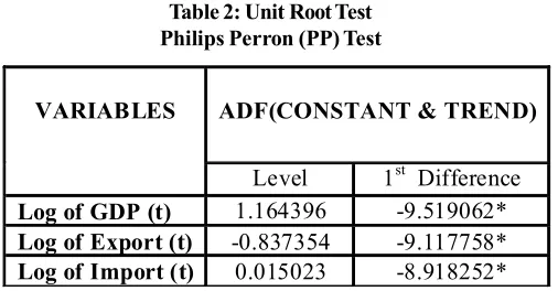
Table 2: Unit Root Test Philips Perron (PP) Test

VARIABLES ADF(CONSTANT & TREND)

Level 1st Difference

Log of GDP (t) 1.164396 -9.519062*

Log of Export (t) -0.837354 -9.117758*

Log of Import (t) 0.015023 -8.918252*

Notes: Superscripts * indicate rejection of null hypothesis at 1% significance.

It is clear from table 1 and 2 that all the data are non stationary at level but they are stationary at first difference.

(7)

cannot. The number of lags depends on Akaike Information criterion. The Granger Causality test can be expressed as:

(1) Log GDP (t) = k₁

i i



Log Export (t-i) + k₁

i i



Log GDP (t-i) + Ut

(2) Log Export (t) = k₁

i i



Log Export (t-1) + k₁

i i



Log GDP (t-i) + Ut

(3) Log GDP (t) = k₁

i i



Log Import (t-i) + k₁

i i



Log GDP (t-i) + Ut

(4) Log Import (t) = k₁

i i



Log Import (t-i) + k₁

i i



Log GDP (t-i) + Ut

Direction of

Causality Number of Lags F Value Result

GDP? Export 2 6.56 No Causality

Export? GDP 2 3.03 No Causality

GDP? Import 2 7.90 No Causality

Import? GDP 2 3.31 No Causality

(8)

(1) Residuals [from cointegration regression of GDP on Export]

Ut = Log GDP (t) - [0 + 1 Log Export (t)]

Or

 Ut = 0 + 1t +2 U (t-1) + k₁ i i



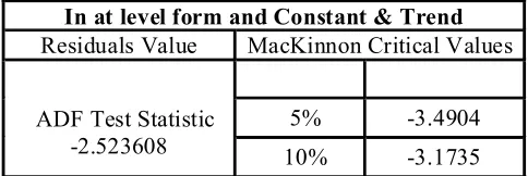
U (t-i)

Table 3: Test for Stationarity of Residuals from Cointegration Regression of Log GDP (t) on Log Export (t)

In at level form and Constant & Trend

Residuals Value MacKinnon Critical Values

ADF Test Statistic -2.523608

5% -3.4904

10% -3.1735

Since the MacKinnon critical values are greater than the value of t-Statistic of Residuals, so the Residuals [from cointegration regression of GDP on Export] is not stationary at level. This empirical content [through the Engel- Granger Representation] leads to conclude that there is not a long run equilibrium relationship between GDP and Export. In other words, GDP and Export are drifting farther from each other in the long run.

(2) Residuals [from cointegration regression of Export on GDP]

Ut = Log Export (t) - [0 + 1 Log GDP (t)]

Or

 Ut = 0 + 1t +2 U (t-1) + k₁ i i



U (t-i)

Table 4: Test for Stationarity of Residuals from Cointegration Regression of Log Export (t) on Log GDP (t)

5% -3.4904

10% -3.1735

(9)

(3) Residuals [from cointegration regression of GDP on Import]

Ut = Log GDP (t) - [0 + 1 Log Import (t)]

Or

 Ut = 0 + 1t +2 U (t-1) + k₁ i i



U (t-i)

Table 5: Test for Stationarity of Residuals from Cointegration Regression of Log GDP (t) on Log Import (t)

5% -3.4904

10% -3.1735

Since the MacKinnon critical values are greater than the value of t-Statistic of Residuals, so the Residuals [from cointegration regression of GDP on Import] is not stationary at level. This empirical content [through the Engel- Granger Representation] leads to conclude that there is not a long run equilibrium relationship between GDP and Import. In other words, GDP and Import are drifting farther from each other in the long run.

(4) Residuals [from cointegration regression of Import on GDP]

Ut = Log Import (t) - [0 + 1 Log GDP (t)]

Or

 Ut = 0 + 1t +2 U (t-1) + k₁ i i



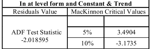
U (t-i)

Table 6: Test for Stationarity of Residuals from Cointegration Regression of Log Import (t) on Log GDP (t)

5% 3.4904

10% -3.1735

(10)

From the table 3, 4, 5 and 6, it is clear that there is no long run equilibrium relationship between GDP, Export and Import because the residuals from these variables are not stationary at the level.

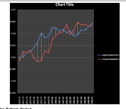
OLS Method: The period between 1970-71 to 1990-91 is called pre reform period and the period between 1991-92 to 2008-09 is called post reform period.

Pre-Reform Period

The elasticity's of export and import with respect to GDP in the table 7

Table 7

Year Export Elasticity’s

Import Elasticity’s 1970-71 0.249967337 0.248515295

1971-72 0.250034827 0.252417496

1972-73 0.252057076 0.252009015

1973-74 0.252398947 0.253065747

1974-75 0.254121544 0.24948579

1975-76 0.256196575 0.248168912

1976-77 0.260383761 0.248395275

1977-78 0.258088766 0.252929101

1978-79 0.258876239 0.251926318

1979-80 0.262491372 0.257226719

1980-81 0.26236879 0.259134606

1981-82 0.26110142 0.260377635

1982-83 0.261949815 0.260635036

1983-84 0.260266239 0.263922218

1984-85 0.261202746 0.259485356

1985-86 0.258867494 0.261790467

1986-87 0.259321926 0.264711731

1987-88 0.261499597 0.263643077

1988-89 0.261358181 0.263853448

1989-90 0.262882372 0.263200417

1990-91 0.264363221 0.262994233

(11)

Pre-Reform Period

The elasticity's of export and import with respect to GDP in the table 8

Table 8

Year Export elasticity's Import Elasticity’s 1991-92 0.249806977 0.146412656

1992-93 0.249912269 0.148335826

1993-94 0.251726664 0.15001361

1994-95 0.253265732 0.151958277

1995-96 0.257872754 0.154355606

1996-97 0.257785494 0.153210607

1997-98 0.256522677 0.15432248

1998-99 0.258122266 0.156003753

(12)

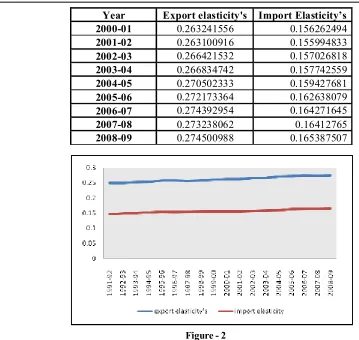
Year Export elasticity's Import Elasticity’s 2000-01 0.263241556 0.156262494

2001-02 0.263100916 0.155994833

2002-03 0.266421532 0.157026818

2003-04 0.266834742 0.157742559

2004-05 0.270502333 0.159427681

2005-06 0.272173364 0.162638079

2006-07 0.274392954 0.164271645

2007-08 0.273238062 0.16412765

2008-09 0.274500988 0.165387507

Figure - 2

In the post reform the export elasticity's is higher than import elasticity. This indicates the policy shifting of Indian government; also this indicates the export substitution policy.

Conclusion

(13)

surprising as India embarked on export-substituting model of growth after independence in 1947 and the reforms of the external sector are more or less a recent phenomenon which is still going on.

References

(1) Abual-Foul, B. (2004). Testing the export-led growth hypothesis: evidence from Jordan. Applied Economics Letters, Vol. 11, pp. 393-396.

(2) Awokuse, T. O. (2005a). Exports, economic growth and causality in Korea, Applied Economics Letters, Vol.12, pp. 693-696.

(3) Awokuse, T. O. (2005b). Export-led growth and the Japanese economy: evidence from VAR and directed acyclic graphs, Applied Economics Letters, Vol.12. pp. 849-858.

(4) Balaguer, J. and Cantavella-Jorda, M. (2001). Examining the export-led growth hypothesis for Spain in the last century. Applied Economics Letters, Vol. 8, pp.681-685.

(5) Balaguer, J. and Cantavella-Jorda, M. (2001). Examining the export-led growth hypothesis for Spain in the last century. Applied Economics Letters, Vol. 8, pp.681-685.

(6) Boriss Siliverstovs & Dierk Herzer, (2007). Manufacturing exports, mining exports and growth: cointegration and causality analysis for Chile (1960--2001). Applied Economics, Taylor and Francis Journals, vol. 39(2), pages 153-167, February

(7) Engle, R. and Granger, C. (1987). Co integration and error correction representation: estimation and testing, Econometrica, Vol. 55, pp. 251-276.

(8) Gujrati, D. (1995). Basic Econometrics, 3rd Edition, McGraw-Hill

(9) Hatemi-J, A. and Irandoust, M. (2000a), Export performance and economic growth causality: an empirical analysis, Atlantic Economic Journal, Vol.28, pp.412-426

Appendix

Table: (` in Crore)

Year GDP Export Import Log GDP Log export Log import 1950-51 224786 606 608 5.351769259 2.782472624 2.783903579

1951-52 230034 716 890 5.361792031 2.854913022 2.949390007

1952-53 236562 578 702 5.373944983 2.761927838 2.846337112

1953-54 250960 531 610 5.399604506 2.725094521 2.785329835

1954-55 261615 593 700 5.417662641 2.773054693 2.84509804

1955-56 268316 609 774 5.428646571 2.784617293 2.888740961

1956-57 283589 605 841 5.452689381 2.781755375 2.924795996

(14)

Year GDP Export Import Log GDP Log export Log import 1958-59 301422 581 906 5.479174947 2.764176132 2.957128198

1959-60 308018 640 961 5.488576097 2.806179974 2.982723388

1960-61 329825 642 1122 5.518283571 2.807535028 3.049992857

1961-62 340060 660 1090 5.53155555 2.819543936 3.037426498

1962-63 347253 685 1131 5.540646006 2.835690571 3.053462605

1963-64 364834 793 1223 5.562095305 2.899273187 3.087426457

1964-65 392503 816 1349 5.593842981 2.911690159 3.13001195

1965-66 378157 810 1409 5.577672144 2.908485019 3.148910993

1966-67 382006 1157 2078 5.582070184 3.063333359 3.317645543

1967-68 413094 1199 2008 5.616048887 3.078819183 3.302763708

1968-69 423874 1358 1909 5.627236778 3.13289977 3.280805928

1969-70 451496 1413 1582 5.654653907 3.150142162 3.199206479

1970-71 474131 1535.3 1634.2 5.675898352 3.18619325 3.213305206

1971-72 478918 1608.2 1824.5 5.68026116 3.206340058 3.261143868

1972-73 477392 1971.5 1867.4 5.678875137 3.294796781 3.271237354

1973-74 499120 2523.4 2955.4 5.698204973 3.401986099 3.470616269

1974-75 504914 3328.8 4518.8 5.703217413 3.522287703 3.65502312

1975-76 550379 4036.3 5264.8 5.740661855 3.605983438 3.721381878

1976-77 557258 5142.7 5073.8 5.746056312 3.71119119 3.705333344

1977-78 598885 5407.9 6020.2 5.777343436 3.733028652 3.779610919

1978-79 631839 5726.1 6810.6 5.800606429 3.757858928 3.833185374

1979-80 598974 6418.4 9142.6 5.777407971 3.807426779 3.961069719

1980-81 641921 6710.7 12549.2 5.807481584 3.826767824 4.098616041

1981-82 678033 7805.9 13607.6 5.831250832 3.892422983 4.133781535

1982-83 697861 8803.4 14292.7 5.843768928 3.944650435 4.155114278

1983-84 752669 9770.7 15831.5 5.876604029 3.989925679 4.199522065

1984-85 782484 11743.7 17134.2 5.893475466 4.069804948 4.233863832

1985-86 815049 10894.6 19657.7 5.911183719 4.03721129 4.293532703

1986-87 850217 12452 20095.8 5.929529784 4.095239112 4.3031053

1987-88 880267 15673.7 22243.7 5.944614421 4.19517153 4.347207029

1988-89 969702 20231.5 28235.2 5.986638291 4.306028083 4.450790868

1989-90 1029178 27658.4 35328.4 6.012490494 4.441827053 4.548123969

1990-91 1083572 32557.6 43192.9 6.034857774 4.512652383 4.635412364

1991-92 1099072 44041.8 47850.8 6.041026144 4.64386506 4.679889203

1992-93 1158025 53688.3 63374.5 6.063717935 4.729879653 4.801914546

1993-94 1223816 69751.4 73101 6.087716127 4.843552929 4.863923318

1994-95 1302076 82674.1 89970.7 6.114636334 4.917369476 4.954101099

(15)

Year GDP Export Import Log GDP Log export Log import 1996-97 1508378 118817.1 138919.7 6.17851019 5.074878948 5.142763837

1997-98 1573263 130100.6 154176.3 6.196801329 5.114279299 5.188017619

1998-99 1678410 139753.1 178331.9 6.224898058 5.14536145 5.251229037

1999-00 1786525 159561.4 215236.5 6.252009098 5.202927838 5.332915921

2000-01 1864301 203571 230872.8 6.270516033 5.30871591 5.36337277

2001-02 1972606 209018 245199.7 6.29504035 5.320183688 5.389519934

2002-03 2048286 255137.3 297205.9 6.311390597 5.406773955 5.473057427

2003-04 2222758 293366.8 359107.7 6.346892182 5.467410964 5.555224717

2004-05 2388768 375339.5 501064.5 6.378173973 5.574424271 5.699893634

2005-06 2616101 456417.9 660408.9 6.417654507 5.659362668 5.819812917

2006-07 2871120 571779.3 840506.3 6.458051344 5.757228429 5.924540973

2007-08 3129717 655863.5 1012312 6.495505069 5.816813462 6.005314256