Green-Based Generation Expansion Planning For
Kenya Using Wien Automatic Software Package
(WASP) IV Model.
Patrobers Simiyu
Institute of Energy & Environmental Technology (IEET); Jomo Kenyatta University of Agriculture & Technology; Nairobi, Kenya Email: [email protected]
ABSTRACT: In 21st Century, there is growing interests in the global power generation sector to integrate more renewable energy (RE) resources in least-cost generation expansion planning for security of supply and sustainable development. However, little has been done in Kenya yet she was endowed with enormous unexploited RE resources. For this reason, the study derived an optimal green least-cost generation expansion plan (OGLCGEP) taking 2010 as the base year to 2031 using the WASP IV model. The study findings showed that the OGLCGEP had a capacity of 1382MW at a peak demand of 1227MW in the base year. However, annual RE capacity additions over the planning horizon will raise the capacities to 19828MW at a peak demand of 16905MW in the reference demand forecast scenario (RDFS) and 26968MW at a peak demand of 22985MW in the higher demand forecast scenario (HDFS). Consequently a 71% to 78% green generation would be realized with 1.94 -3.02 % LOLP. Additionally, the envisaged RE system would supply 7721GWh to 105766 GWh in the RDFS and 143830GWh in the HDFS with a cumulative total of 18 to 23.6Mt CO2 emissions. Moreover, the energy system’s cost would be US$ 14.62 billion in the RDFS; US$ 5.34 billion higher in the HDFS by 2031. Subsequently, the system’s net present value would be US$ +2.16 billion in the RDFS; US$ +4.92 billion higher in the HDFS besides potential carbon credits. Thus, the OGLCGEP would be a feasible option and the future for high RE grid integration for Kenya. Therefore, the research recommends future studies to focus on modeling of the Kenya national-grid reliability and stability with high penetration of variable renewable energy sources.
Keywords :Generation Expansion Planning; Renewable energy; WASP IV; Optimal Solution; Senstivity Analysis; CO2 emissions; net present value
1.0
I
NTRODUCTIONThe world power generation sector is projected to undergo unprecedented demand growth from 17,408 TWh in 2004 to 33,750 TWh in 2030 at an average annual growth rate of 2.6%. To meet this demand, the sector will built 5,087GW of which over 75% will come from oil, coal and gas power plants. Consequently, the carbon-intensive plants are expected to rise the CO2 emissions from 9600-16400Mt at an annual growth rate of 2%. The rapidly increasing global emission is the major cause of global climate change [1]. Consequently, the global generation sector is faced with enormous pressure to lead the way in climate change mitigation strategies. Thus generation companies (GENCOs) in many countries in the world are currently planning towards environmentally-friendly generation investments [1], [2]. The most popular energy policy measure towards this course is the use of Renewable energy (RE) as suitable clean energy option to the conventional carbon intensive plants [3], [4]. Subsequently, more integration of RE in the power system’s least-cost generation expansion planning (GEP) is rapidly gaining extraordinary consideration as a sustainable option to security of power and CO2 emission reduction [5], [6]. The system integration also presents a significant potential for carbon credits as revenues in the generation sector from the carbon market [7], [8], [9]. Furthermore, other fringe benefits such as health benefits, green jobs and foreign exchange savings prevail for sustainable development [10], [11]. In Kenya, the generation sector prepares 20 year rolling least cost power development plan (LCPDP) at the energy regulatory commission (ERC) for expanding the power system to meet the current and future power demands. The 2011-2031 LCPDP under the focus of this study had projected a hydropower and heavy fuel oil (HFO) dominated power generation [12] that posed serious challenges. The hydros were vulnerable to acute energy shortfalls due to the frequent droughts. On the other hand, the HFO and the planned conventional coal plants posed the CO2 emissions dilemma [13], [14]. These were crucial issues for
2.0
M
ETHODOLOGY2.1WIEN AUTOMATIC SYSTEM PLANNING (WASP)IV
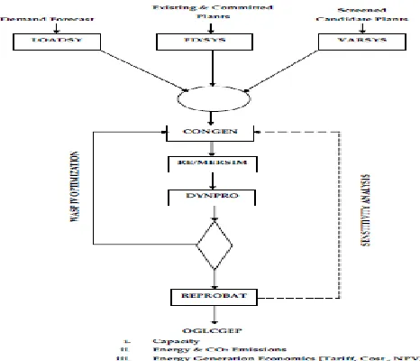
The Wien Automatic software package (WASP) is the most frequently used and best proven model for GEP analysis worldwide. It is developed and maintained by the International Atomic Energy Agency (IAEA) for free to its member states. WASP IV model is the fourth versions of WASP have been developed and distributed worldwide [19], [25]. It is systematic and modular consisting of various modules and associated files. Suitable batch files are provided in the model for executing different modules. However, correct input data should be provided for each module for creating input files prior to the execution process [19], [20]. The first three modules are for basic input data on the demand forecast, candidate generation plants as well as committed plants. These include; load system (LOADSY), fixed system (FIXSYS) and variable system (VARSYS) respectively. The three modules are executed independently of each other. The next four modules namely; configuration generator (CONGEN), merge and simulate (MERSIM), Re-merge and simulate (REMERSIM) and dynamic programming (DYNPRO) are executed after analyzing the first three. The WASP IV model is accomplished with powerful attributes to address new and emerging issues in the generation sector in late 1990s [19], [21]. The new features incorporated include: • Options for environmental emissions, fuel usage and energy generation constraints
• Representation of pumped-storage plants • Fixed maintenance schedule
• Environmental emission calculations
• Expanded capabilities for handling up to 90 plants types and
500 configurations per year. The model attributes designed in an enhanced dynamic programming (DP) algorithm incorporated with heuristic technique is capacable of deriving the optimal solution for generation capacity addition that meets the energy demand for at most 30 years. Fundamentally, the evaluation of the optimal solution is based on minimizing the objective cost function that represents the generation energy system’s cost that consists of the existing and candidate plants. The objective function is defined as the sum of the construction costs, operation & maintenance costs (including fuel costs) and the cost of energy not served, less the salvage value of the generation investment. These cost function is subject to reliability, tunnel (construction), fuel availability and emission constraints [16], [21], [25]. In the WASP IV model, the system’s costs are simulated through probablistic product cost (PPC) besides the generation costs, cost of energy not served and reliability (LOLP). The linear programming is used in establishing the optimal generation dispatch plan that fulfills environmental emissions, fuel availability and energy generation (by some plants) constraints. Subsequently, the enhanced DP optimization evaluates the costs of the alternative system expansion policies and derives the optimum solution [19]. The PPC technique is affirmed by [20], [22] as the best analytical framework that GENCOs use when evaluating generation cost taking risks into account. However, the generation projects are capital intensive and often stay for long hence their financial flows occur after some years. Hence, present valuing (discounting) of their costs and benefits to their PV enable proper project evaluation. A choice of a proper discount rate cushions inflation and other investment
uncertainties [5], [21], [25], [26]. As a matter of fact, discounting (time value of money) has featured widely in literature for evaluating power generation projects. In this way, reliable financial techniques such as the net present value (NPV), future worth value (FWV) and internal rate of return (IRR) are applied extensively. The NPV is the most effective financial project evaluation technique [14], [23], [26]. Additionally, the economics of system generation reliability often strike a balance between cost and quality of service. Typically, the long-run marginal cost (LRMC) is the levelised cost where the marginal utility for the extra reliability enhancement to the consumer equals the marginal cost spent by the power supplier. In this way, the LRMC serves as the basis for establishing the electricity tariffs [5], [26], [24]. Therefore, the impressive simulation and optimization features in WASP IV model has made it a popular tool for solving many GEP problems in various countries around the world [25], [21], [26].
2.2MODELING THE OGLCGEP
Figure 1: WASP IV GEP Methodology
The optimization process minimized certain cost components in the objective cost function in DYNPRO discounting the energy system’s cost at an 8% discount rate subject to capacity, technology and operational constraints. The objective function (Bj) represented by the equation (1) is composed of:
capital investment costs (I), fuel costs (F), operation and maintenance (O&M) costs (M), fuel inventory costs (L), salvage value of investments (S) and cost of energy demand not served (ø). The planning period of time (t) was given in years while T (22) was the length of the study period in years.
(1)
2.3OGLCGEPCO2EMISSIONS
The CO2 emissions for the OGLCGEP in the RDFS and the HDFS were determined using the emission factors from the 2014 US Climate Registry. In each scenario, the energy technologies considered varied in the emission factors based on their environmental pollution extents. Table 1 displays the emission factors for the energy generation technologies considered in the study.
Table 1: Emission Factors for Energy Generation Technologies
SNo. Energy Technology TonCO2/GWh
1 Baggase 301.8014
2 Kerosene 246.8583
3 HFO 249.7988
4 Natural gas 181.2356
5 Geothermal 25.6918
The annual CO2 emission for the given energy technology in the planning period was computed using equation (1).
(2) The total CO2 emission for each technology in the period was
established as the sum of the annual emissions in each scenario.
2.4OGLCGEPGENERATION ECONOMICS
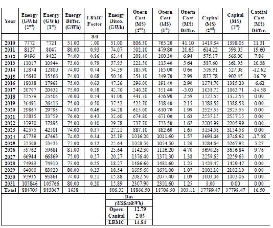
Most economic costs of generation for the OGLCGEP were directly in the energy system’s cost function in equstion 1. However, the average cost per unit generated was determined indirectly using the long-run marginal cost (LRMC); the most convenient approach for calculating power tariffs recognized by IES, (2004). In the LRMC, two optimal generation programs were considered in the WASP IV. The first program was essentially the OGLCGEP derived for the given demand forecast (RDFS or HDFS) while the second under an incremental load on the demand forecast. The REPROBAT results on the energy, operation cost and capital cost for each program was utilized to generate a LRMC model in Microsoft Excel for the planning period. Additionally, the corresponding energy, operation cost & capital cost differences; LRMC factors (0.20 to 1.00) and energy discounts comprised essential LRMC model constituents. Fig 2 shows the LRMC model for the OGLCGEP.
Figure 2: LRMC Model for the OGLCGEP
The energy discount was computed using equations (3). Additionally, the operation and capital cost differences were crucial in the LRMC calculation at the bus as shown in equations (4).
(3)
(4)
Consequently, the PV inflows were calculated using equation (5) and the net present value (NPV) as the long-term future revenues for the OGLCGEP determined using equation (6).
(5)
(6)
2.5OGLCGEPSENSITIVITY ANALYSES
OGLCGEP. Therefore, the study involved varying each of the given economic factors in DYNPRO at definite steps for the RDFS and the HDFS. Thus, the discount rate was varied from 8% to 12% in steps of 2%; the fuel cost from 10% to 30% in steps of 10% and finally the capital cost from 5% to 15% in steps of 5%. A re-run of DYNAPRO was undertaken where the variations retained the OGLCGEP within its initial CONGEN tunnel boundaries. However, in cases where the changes blew the tunnel boundaries, few CONGEN iterations and CONGEN-MERSIM-DYNPRO re-runs were executed to attain a new unconstrained OGLCGEP.
3.0
R
ESULTS3.1REFERENCE DEMAND FORECAST SCENARIO(RDFS)
3.1.1CAPACITY MIX
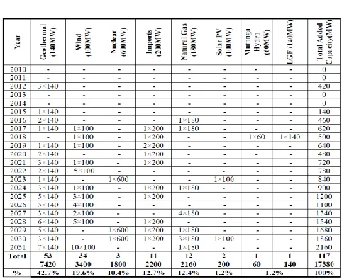
The optimal solution of adding new capacities annually for the selected RE candidate plants was obtained for the 2011-2031 planning period. The capacity additions were derived taking into account the technical, economic and environmental constraints that directly influenced availability of candidates for capacity addition. Table 2 presents the RE capacity addition schedule in the RDFS. The results show that the initial capacity addition will be 420MW from geothermal. This will be increased gradually to17380MW by 2031. In total, geothermal will have the highest additions at 42.7%. The least will be from hydro and solar PV each at 1.2%.
Table 2: OGLCGEP RE Capacity Addition Schedule (MW) – RDFS
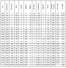
When the RE capacity additions were integrated in the exiting generation system; the OGLCGEP capacity in the RDFS was derived as shown in table 3 and fig 3. The results show that the generation capacity was 1382MW at a peak demand of 1227MW in the base year. This was predominated by hydropower (55%) and HFO (24%). In comparison to the rest of the planning period, the generation system had the least reserve capacity hence the highest LOLP of 23.3%. The rising RE capacity additions at an average rate of 901MW per annum projected to vary the system’s capacity in the base year to 19828MW at 16905MW peak demand in 2031. The generation capacities would be characterized by low LOLPs averaged at 1.94%. By 2031, the generation capacity would be
78% green and dominated by geothermal (40.8%) wind (19.2%).
Table 3: OGLCGEP Capacity (MW) – RDFS
Figure 3: OGLCGEP Capacity (MW) – RDFS
3.1.2ENERGY AND CO2EMISSIONS
Figure 4: OGLCGEP Energy Mix (GWh) – RDFS
Consequently, the energy system would emit some CO2 emissions over the planning period. Fig 5 illustrates the profile for the CO2 emissions for the OGLCGEP in the RDFS. The results show that the annual emissions would grow from 0.73 Mt CO2 in the base year to 2 Mt CO2 in 2031. In the base year, HFO would be the highest emitter at about 77.8% of the total. However the trend would depart to majorly geothermal with increasing annual RE supply additions over the planning period by 2031. By the end of the planning period, a cumulative total of 18Mt CO2 at the average rate of 0.82 Mt CO2 per year would be emitted. Geothermal will be the highest emitter at 77% of the total. Other RE such as hydropower, wind and solar PV will have any emissions.
Figure 5: OGLCGEP CO2 Emission – RDFS
3.1.3GENERATION ECONOMICS
The average power tariff per unit generated for the OGLCGEP
was determined as US$cts 14.84/kWh. Table 4 shows the OGLCGEP long-run marginal cost (LRMC) in the RDFS. The generation companies (GENCOs) would use the LRMC as an average tariff for selling power to the power distribution company. The rate would determine their present value (PV) inflows from power generation.
Table 4: OGLCGEP LRMC – RDFS
On the other hand, the optimal energy system’s cost for the OGLCGEP was determined as US$ 14.62 billion with a salvage value of US$ 1.09 billion by 2031. This would be the minimum possible generation system’s cost minimized in the overall objective cost function in the WASP IV model. Subsequently, the net present value (NPV) for the OGLCGEP was determined as US$ 2.16 billion at the optimal energy system’s cost. Table 5 present the financial flows of the OGLCGEP for the RDFS. The results show that the NPV would grow towards positive as the system tends towards 2031. In fact, it would break even around 2029-2030.
3.2HIGHER DEMAND FORECAST SCENARIO (HDFS)
3.2.1CAPACITY MIX
The optimal solution in the HDFS was obtained with higher proportions of RE capacity additions in comparison to the RDFS. Table 6 presents the annual RE capacity addition schedule in the HDFS. The results in table show that all candidate plants except imports and hydropower will increase with reference to the RDFS during the planning period. The RE generation capacities will be added as follows relative to the RDFS; geothermal 7420MW to 9940MW; wind 3400MW to 4500MW; nuclear doubled from 1800MW; natural gas from 2160MW to 3780MW and solar PV 200MW to 300MW. In consequence, the total RE capacity additions of 17380MW (RDFS) will increase to 24520MW (HDFS). On aggregate, geothermal at 40.5% will account for the highest total capacity additions while hydropower at 0.8% the least.
Table 6: OGLCGEP RE Capacity Addition Schedule (MW) – HDFS
The OGLCGEP capacity in the HDFS was derived as shown in table 7. The results show that the generation capacities were entirely the same as the RDFS for the base year. However, the rising annual RE capacity additions at an average rate of 1226MW would vary the generation capacity to 26968MW at peak demand of 22985MW in 2031. This would be relatively higher than the corresponding 19828MW capacity at 16905MW peak demand in the RDFS. The capacities in the HDFS would demonstrate higher annual LOLPs averaged at 3.02% as opposed to 1.94% for the RDFS. By 2031, the generation capacity would 71% green and dominated by geothermal (39.4%) and wind (18.5%) of the total.
Table 7: OGLCGEP Capacity (MW) – HDFS
3.2.2ENERGY MIX AND CO2EMISSIONS
The OGLCGEP energy for the HDFS would be capable of meeting the prevailing demand over the planning horizon. Fig 6 presents the OGLCGEP energy mix in the HDFS. The results show that the energy mix would increase from 7721 GWh in the base year to 143830GWh in 2031. This will be higher than the corresponding system’s energy of 105766GWh in the RDFS.
Figure 6: OGLCGEP Energy (GWh) – HDFS
0.73 Mt CO2 in the base year same as in the RDFS to 2.9 Mt CO2 in 2031. However, the varying RE supply additions from the RDFS resulted in a cumulative total of 23.6Mt CO2; 5.6 Mt CO2 higher than the RDFS to be emitted by 2031. Similarly, geothermal would be the highest emitter at 73.7% of the total as in the HDFS. Moreover, like in the RDFS, Other RE such as hydropower, wind and solar PV would have no emissions at all.
Figure 7: OGLCGEP CO2 Emission – HDFS
3.2.3GENERATION ECONOMICS
The average power tariff per unit generated was determined as US$cts 17.85/kWh /kWh. Table 8 shows the OGLCGEP LRMC in the HDFS. The results GENCOs would sell power to power distributing companies at an average of US$cts 3.01/kWh higher in the HDFS than in the RDFS. As a result, the rate would depict higher present value (PV) inflows from power generation than in the RDFS.
Table 8: OGLCGEP LRMC – HDFS
Conversely, the optimal energy system’s cost for the OGLCGEP was determined as US$ 19.96 billion at a salvage
value of US$ 1.37 billion by 2031 in the HDFS. In this case, the system’s cost was US$ 5.34 billion higher than the RDFS. Subsequently, the NPV for the OGLCGEP was US$ 7.08 billion at the optimal energy system’s cost; US$ 4.92 billion higher than the RDFS. Table 9 present the financial flows of the OGLCGEP for the HDFS. The results show that the NPV would grow towards positive as the system tends towards 2031 similar to the RDFS. In fact, it would break even around 2027-2028 but a year earlier than the RDFS.
Table 9: OGLCGEP Financial Inflows & Outflows – HDFS
3.3THE OGLCGEPSENSITIVITY ANALYSES
3.3.1VARIATIONS IN DISCOUNT RATE ON SYSTEM’S COST AND
NPV OF THE OGLCGEP
When the discount rate was varied between 8% and 12%; the energy system’s cost of the OGLCGEP decreased while NPV increased in the RDFS and HDFS. Table 10 shows the variations in the discount rate on system’s cost and NPV of the OGLCGEP. The results show that the system’s cost will decrease at the rate of US$ 0.97 to US$ 1.34 billion per % discount rate increase in the RDFS and HDFS respectively. Conversely, the NPV will increase at a lower rate of US$ 0.82 to US$ 1.15 billion per % discount rate increase in the RDFS and HDFS respectively. Despite these discount rate variations, the total number of generation plants remained unchanged in both scenarios.
Table 10: Variations in Discount Rate on System’s Cost and NPV of the OGLCGEP
3.3.2VARIATION IN FUEL COST ON SYSTEM’S COST AND NPV OF THE OGLCGEP
increased slightly whereas the NPV reduced marginally. Table 11 shows variations in fuel cost on system’s cost and NPV of the OGLCGEP. The results show that the system’s cost will increase at the rate of US$ 0.03 to US$ 0.07 billion per % fuel cost increase in the RDFS and the HDFS respectively. Similarly at the same rate as the above system’s cost increase, the NPV will decrease in both scenarios. In spite of these fuel cost variations, the total number of plants remained constant in both scenarios.
Table 11: Variations in Fuel-Cost on System’s Cost and NPV of the OGLCGEP
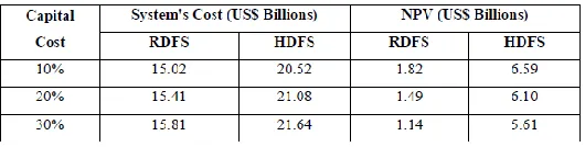
3.3.3VARIATIONS IN CAPITAL COST ON SYSTEM’S COST AND NPV
OF THE OGLCGEP
When the capital cost was increased by 5% to 15%, the energy system’s cost of the OGLCGEP narrowly increased while the NPV decreased slightly in each scenario. Table 12 shows the variations in capital cost on system’s cost and NPV of the OGLCGEP. The results show that the capital cost will increase at the rate of US$ 0.2 to US$ 0.28 billion per % increase in the RDFS and the HDFS respectively. On the contrary, the NPV will decrease at a lower rate of US$ 0.17 to US$ 0.25 billion per % increase in the RDFS and the HDFS respectively. Despite these capital cost variations, the total number of plants remained the same in both scenarios.
Table 12: Variations in Capital Cost on System’s Cost and NPV of the OGLCGEP
4.0
D
ISCUSSIONSThe OGLCGEP generation capacity was projected to grow from 1382MW at 1227MW peak demand in the base year to 19828MW at a peak demand of 16905MW in the RDFS and 26968MW capacity at a peak demand of 22985MW in the HDFS. In the base year, the generation capacity was predominantly hydropower in both scenarios. It was 55% hydropower and 24% HFO with the least reserve capacity hence the highest LOLP of 23.3%. However, the RES capacity additions over the planning horizon changed the entire generation portfolio. In the RDFS, the generation capacities would be 78% green and dominated by geothermal (40.8%) wind (19.2%) by 2031. Additionally, the capacities would characterized by low annual LOLPs averaged at 1.94% over the planning horizon. In the HDFS, the generation capacities would 71% green and predominantly geothermal (39.4%) and wind (18.5%) by 2031. However, the capacities would be characterized by relatively higher annual LOLPs of 3.02% on average. According to [5] and [20]; high LOLP(s) portrayed low generation reliability to meet the requisite demand.
fuel cost showed unique effect on the system’s cost and NPV. In this case, an increase in the fuel cost showed that the energy system’s cost would increase at the rate of US$ 0.03 to US$ 0.07 billion per % fuel cost increase in the RDFS and the HDFS respectively. By way of contrast, the NPV robustly decreased at exactly the same rate as the above system’s cost increase in each scenario. Yet, an increase in fuel cost would significantly escalate the energy system’s cost over the NPV as remarked by [25], [26]. Contrastingly, the OGLCGEP was less sensitive to fuel cost rise because of its majorly fuel-free RE power generation similar to those indicated in [4]. Despite the discount rate, fuel cost and capital cost variations; the total number of plants remained constant in both scenarios. This was another striking indicator of the RE system’s stability to variation in economic parameters.
5.0
C
ONCLUSIONS ANDR
ECOMMENDATIONThe derived optimal green least cost generation expansion plan (OGLCGEP) will have the generation capacity of 1382MW at 1227MW peak demand in the base year to 19828MW at a peak demand of 16905MW in the RDFS and 26968MW capacity at a peak demand of 22985MW in the HDFS by 2031. In the RDFS, the generation capacities would be 78% green and dominated by geothermal (40.8%) wind (19.2%) by 2031 and characterized by a modest annual reliability averaged at 1.94% LOLP. In the HDFS, the generation capacities would 71% green and predominantly geothermal (39.4%) and wind (18.5%) by 2031 with relatively higher annual LOLPs of 3.02% on average. On the contrary, the planned energy system for the OGLCGEP would supply 7721GWh in the base year to 105766 GWh in the RDFS and 143830GWh in the HDFS by 2031. Consequently, the energy system’s cumulative total of 18 and 23.6Mt CO2 emissions in the RDFS and HDFS respectively presenting a business opportunity from carbon credits tradable as market revenues for green generation growth in Kenya through the clean management mechanisms (CDM). In addition , the planned energy system’s cost consisting of the existing and the candidate generation plants for the OGLCGEP was projected to be US$ 14.62 billion in the RDFS; US$ 5.34 billion higher in the HDFS by 2031. Subsequently, the energy system’s NPV would be US$ +2.16 billion in the RDFS; US$ +4.92 billion higher in the HDFS by 2031 besides potential carbon credits. For this reasons, the envisaged energy system would be a viable generation investment hence the future for higher RE grid integration for Kenya. Therefore, the research recommends future studies to focus on modeling of the Kenya national-grid reliability and stability with high penetration of variable renewable energy sources.
A
CKNOWLEDGMENTI would like to thank Dr. Oliver Johnson of the Stockholm Environmental Institute (SEI); Nairobi for his mentorship during the preparation of this paper. I also acknowledge the support provided by the SEI Write-shop to Support Developing of Country Publications on Transitions to Modern Energy Systems in which this paper was chosen. I declare that there was not conflict of interest in this research.
R
EFERENCES[1] IPCC. (2013). Working Group I Contribution to the IPCC Fifth Assessment Report, Climate Change
2013: Physical Science Basis, Summary for Policy Makers. Online at:http://www.ipcc.ch/
[2] IPCC. (2011). Renewable Energy Sources and Climate Change Mitigation; Summary for PolicyMakers and Technical Summary. Online
at:http://www.ipcc.ch/pdf/special-reports/srren/SRREN_FD_SPM_final.pdf
[3] Mejía Giraldo, Diego Adolfo, López Lezama, Jesús María, Gallego Pareja, Luis Alfonso. (2012). Power System Capacity Expansion Planning Model Considering Carbon Emissions Constraints; Revista Facultad de Ingeniería Universidad de Antioquia.
Online at:
http://www.redalyc.org/articulo.oa?id=43025115012 ISSN 0120-6230
[4] REN21. (2014). Renewables 2014 Global Status Report. Renewable Energy Policy Network forthe 21st
Century. Online at:
http://www.ren21.net/Portals/o/documents/
/Resources/GSR/2014/GSR2014_full%20report_low %20res.pdf
[5] Kathib, H. (2003). Economic Evaluation of Projects in Electricity Supply Industry. The Institution of Electrical Engineers, London, UK.
[6] Maslyuk, S and Dharmaratna. (2013). Renewable Electricity Generation, CO2 Emissions and Economic Growth: Evidence from Middle-Income Countries in Asia. Estudios De Economia Aplicada. Vol. 31 – 1 pp. 217 – 244.
[7] Gupta, Yuvika. (2011). Carbon Credit: A Step towards Green Environment. Global Journal of Management & Business Research, 11(5)1.0, April 2011.
[8] Shende, B.R. and Jadhao, R.S. (2014). Carbon Credit Science and Business. Science Reviews & Chemical Communications, 4(2),pg. 80-90. Online atwww.sadgurupublications.com
[9] Sukumaran, A.K.S. (2014). Carbon Trading and Green House Gas Emission - An Analysis. Asian Journal of Scientific Research, 7(3), pg. 405-411.
Online at
http://scialert.net/abstract/?doi=ajsr.2014.405.411
[10]UNEP. (2008). Green Jobs; Towards Decent Work in a Sustainable, Low-Carbon World. Online at http://www.unep.org/PDF/UNEPGreenjobs_report08.p df
[11]UNEP. (2011). Towards Green Economy; Pathways to Sustainable Development and Poverty Eradication – A Synthesis for Policy Makers. Online at http://www.unep.org/greeneconomy/Portals/88/docum ents/ger/GER_synthesis_en.pdf
[13]MEWNR. (2014). National Climate Change Framework Policy. Nairobi: Ministry of Environment, Water & Natural Resources.
[14]MOE. (2013). National Energy Policy. Nairobi: Ministry of Energy.
[15]Kengen. (2013). 61st Annual Report & Financial Statements; Financial Year Ended 30th June 2013, Nairobi: Kenya Generation Company.
[16]Ondracnek, J. (2014). Are we there yet? Improving Solar PV Economics and Power Planning in Developing Countries: A Case-Study of Kenya. Renewable & Sustainable Energy Reviews 30: 604 – 615.
[17]SWERA. (2008). Kenya Country Report; Solar and Wind Energy Resource Assessment. Nairobi. Online at:
http://www.unep.org/eou/Portals/52/Reports/SWERA_ TE_Final Report.pdf
[18]Simiyu, Patrobers. (2015). Screening Power Plants for Green-Based Generation Expansion Planning for Kenya. On line at http://www.iosrjournals.org/iosr-jeee/pages/check-paper-status.html (submitted for publication)
[19]IAEA. (2006). Wien Automatic System Planning (WASP) Package: A Computer Code for Power Generating System Expansion Planning, Version WASP-IV with User Interface User’s Manual. Vienna.
[20]IAEA. (1984). Technical Reports Series No. 241; Expansion Planning for Electrical Generating Systems: A Guidebook, International Atomic energy
Agency. Online at:
http://www.energycommunity.org/documents/IAEATR S241.pdf
[21]Elkarmi, F. and Abu-Shikhah, N. (2012). Power System Planning Technologies & Applications: Concepts, Solutions and Management . Engineering Science Reference (IGI Global). ISBN 978-1-4666-0174-1 (ebook). Online athttp://www.igi-global.com
[22]Fabien A. R, Nuttal, W.J., Newbery D. M. (2006). Using Probabilistic Analysis to Value Power Generation Investments Under Uncertainty. Electricity Policy Research Group, University of Cambridge, England.
[23]Stoft, S. (2002). Power System Economics; Designing Markets for Electricity. IEEE Press & Wiley-Interscience. ISBN 0-471-15040-1
[24]Intelligent Energy Systems (IES). (2004). The LRMC of Electricity Generation in New South Wales. A Report to the Independent Pricing & Regulatory Tribunal. Online at: http://www.ipart.nsw.gov.au
[25]Bhattachryya S.C and Tamilsna, G. (2010). A Review
of Energy Systems Models. International Journal for Energy Sector Management Vol 4, No.4. Emerald Group Publishing Ltd. Online at: http://www.ewp.rpi.edu/hartford/~ernesto/S2013/MME
ES/Readings/W01/Bhattacharyya2010-ReviewEnergySystemModels.pdf
[26]Bhattacharyya, S.C. (2011). Energy Economics Concepts Issues, Market & Governance. Springer Verlag London Ltd. UK (e-ISBN 978-0-85729-268-1)
---
AUTHOR