Single image super-resolution by directionally structured coupled dictionary learning

R E S E A R C H

Open Access

Single image super-resolution by

directionally structured coupled

dictionary learning

Junaid Ahmed

and Madad Ali Shah

Abstract

In this paper, a new algorithm is proposed based on coupled dictionary learning with mapping function for the problem of single-image super-resolution. Dictionaries are designed for a set of clustered data. Data is classified into directional clusters by correlation criterion. The training data is structured into nine clusters based on correlation between the data patches and already developed directional templates. The invariance of the sparse representations is assumed for the task of super-resolution. For each cluster, a pair of high-resolution and low-resolution dictionaries are designed along with their mapping functions. This coupled dictionary learning with a mapping function helps in strengthening the invariance of sparse representation coefficients for different resolution levels. During the

reconstruction phase, for a given low-resolution patch a set of directional clustered dictionaries are used, and the cluster is selected which gives the least sparse representation error. Then, a pair of dictionaries with mapping functions of that cluster are used for the high-resolution patch approximation. The proposed algorithm is compared with earlier work including the currently top-ranked super-resolution algorithm. By the proposed mechanism, the recovery of directional fine features becomes prominent.

Keywords: Coupled dictionary learning, Compact directional dictionaries, Sparse representations

1 Introduction

Super-resolution (SR) is the goal in image data presenta-tion which is already an active area of research for some years due to the interest in high-resolution (HR) images in many applications. Of course, HR images can easily be generated by using a high-definition (HD) camera. For some applications, it is still not yet practical to install such a camera (e.g., due to limitations of the capacity of the data channel), or simply not cost-efficient in a particular context of computer vision, medical imaging, or satellite imaging.

Recently proposed image representation approaches use sometimes sparse representation models for storage or transmission reasons. According to the so-called Sparse-land model [1], a set of signals called the dictionary is created for linearly representing the signals of inter-est. These dictionaries are designed by selecting image

*Correspondence: [email protected] Sukkur Institute of Business Administration, Sukkur, Pakistan

patches from a natural set of images and iteratively min-imizing the representation error. Sparsity is used as the regularizing technique (for achieving SR image represen-tations) by enforcing the concept that low-resolution (LR) projections are preserved in linear relations of their HR counterparts [2].

Earlier dictionary learning algorithms for super-resolution were focused on learning the separate HR and LR dictionaries for super-resolution. In [3], authors propose a joint dictionary learning mechanism for learning HR and LR dictionaries in a joint feature space, thus enforcing the similarity between HR and LR sparse coefficients. At the image reconstruction, stage authors proposed the invariance of sparse coefficients for HR and LR patches. In [4], authors propose a multi-scale dictio-nary learning approach where wavelets were used for analysis of the LR images and dictionaries were learned at different resolution levels. By doing so, authors designed compact dictionaries at different resolution levels achiev-ing reduced computational cost. In [5], authors propose multi-scale dictionary learning by introducing local

and non-local priors for the task of single-image super-resolution. These priors are used to recover SR images by suppressing artifacts and estimating the required HR image pixels. However, in the recent work, authors propose the use of classification of training data based on scale invariant features and learn the class-dependent dictionaries instead of a single universal one or on multi-scales.

Related work includes Dong et al. [6] where authors proposed to divide the training data by k-means algo-rithm and clustered data into different sets and then applied the dictionary learning to get the compact dictio-naries. In [7], Feng et al. use k-subspace clustering and divided the data into different subspaces and then dic-tionaries were learned from those subspaces in a shared bases manner. More recently, Yu et al. [8] consider the design of structural dictionaries. In [8], authors consid-ered the orthogonal bases for the dictionary atoms and designed structured dictionaries from those orthogonal bases. Yang et al. [9] propose the use of multiple patches based clustered dictionaries instead of a single universal one. In this mechanism, the authors studied the geomet-ric properties of the image patches. Patches were clustered into different clusters depending on their geometric prop-erty. Dictionaries were obtained from training the image patches from these clusters. In [10], authors designed nine LR directional dictionaries for solving the single-image SR problem. Here, the LR dictionaries were learned by the K-SVD algorithm [1] and HR dictionaries were obtained by solving a pseudo-inverse problem. An important thing to note here is that despite clustering the data into the direc-tional templates, in the dictionary learning process there is no coupling between the HR and LR sparse represen-tation coefficients. Because the SISR problem depends on the invariance of the sparse coefficients. The idea of single dictionary learning with no coupling between the sparse coefficients has already been superseded by [11, 12].

In [12], the authors proposed a coupled dictionary learning mechanism for training of HR and LR dictionar-ies. In this setup, an alternate mechanism is applied to the sparse coefficients of HR and LR patches; for each itera-tion, one sparse coefficient is chosen either the HR or LR and it is used to update both the HR and LR dictionar-ies. In doing so, authors achieved a slight improvement in forcing the sparse coefficients of HR and LR to be the same and thus produced results on par with the state-of-the-art algorithm published in [11].

In this paper, for the task of SISR, the basic idea of Yang et al.’s [11], the approach is assumed that the HR and LR have the same sparse coefficients. Instead of using a sin-gle pair of dictionaries as done in [11] and [12], multiple directional dictionaries are proposed as done in [10]. The training data is divided into eight directional clusters and a non-directional one. The training data is clustered by

correlating the training patches with already developed directional templates. These templates have directional structure. It is shown that these are helpful in creating compact and directional dictionaries.

Now for each cluster, a pair of directional and compact dictionaries are designed along with their mapping func-tions. In the image recovery stage, each patch at hand is recovered with each cluster dictionary by calculating the sparse representations and using the already designed HR dictionary and mapping functions. Then, based on the sparse representation error, a proper dictionary pair is selected along with a mapping matrix. Sparse coefficients are calculated for the LR patch using the selected LR dic-tionary and mapping matrix. Then, HR patches are recon-structed by using the sparse representation along with the corresponding HR dictionary and mapping matrix. This clustering mechanism, along with the mapping function paradigm, allows us to super-resolve patches with high-frequency components. Experiment results show that the proposed algorithm is on par with the existing state-of-the-art algorithms and shows improvement in recovering images with directional fine features.

The rest of the paper is structured as follows. Section 2 presents the super-resolution via sparse representations. Section 3 describes the proposed algorithm. Section 4 reports simulations. Section 5 concludes. Section 5.1 gives future recommendations.

2 Image super-resolution

Achieving SISR is a type of problem that is ill-posed. Researchers tried to regularize the solution process. Recently, authors proposed a very effective method called sparsity, for regularization. Sparsity has a very nice prop-erty of scale invariance (to some extent) due to resolution blur [11]. Using sparsity as a regularizer, one can find HR from LR images using the scale invariance of sparse coefficients.

LetxH be the HR signal vector extracted from an HR

image in the form of the 2−Dpatch, then vectorized into column form. Let DH be the corresponding HR

dictio-nary whose columns represent atoms. We can represent this signal vectorxH by using the sparse representations

asxH ≈ DHαH, where αH is a sparse coefficient matrix

for the HR signal vector with only very few non-zero elements.

LetxL be the corresponding LR signal vector extracted

in the same manner after performing blurring and down-sampling operation on the HR images. The sparse repre-sentation of this vector LR signal can be given as xL ≈ DLαL, where DL represents the dictionary for the LR

signal vector and αL represents the sparse coefficient matrix for the LR signal vector.

down-sampling operator applied on HR images to gener-ate the LR signal vectors. Using this operator we can relgener-ate the HR and LR signal vectors. This operation is expressed in Eq. 1. This concept also extends to the sparse repre-sentation of HR and LR signal vectors. Considering the invariance of the sparse coefficients due to resolution blur, we can also relate the HR and LR dictionaries by the same operator. This operation is expressed in Eq. 2.

xL≈ψxH, (1)

DL≈ψDH. (2)

See [11]. It follows that

xL≈ψxH≈ψDHαH ≈DLαL. (3)

From Eq. 3, it is concluded thatαH ≈αL.

This is the background of a key idea for solving the problem of SISR by sparse representations. If xL,DL,

and DH are given, then one can calculate αL by using

some vector selection algorithm either by greedy meth-ods or relaxation methmeth-ods. Finally, the HR patches can be estimated by

xH ≈DHαL. (4)

3 The proposed method

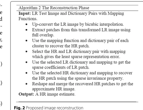
This proposal addresses dictionary learning and image reconstruction by multiple dictionary learning and selec-tive sparse coding, and it is outlined in the algorithms presented in Figs. 1 and 2. During the dictionary learn-ing process, a set of directionally structured dictionar-ies is learned along with a non-directional one. These learned dictionaries along with their inherent mapping functions are used for the reconstruction of the desired images.

Fig. 1Proposed dictionary learning algorithm

Fig. 2Proposed image reconstruction

3.1 The proposed dictionary learning algorithm

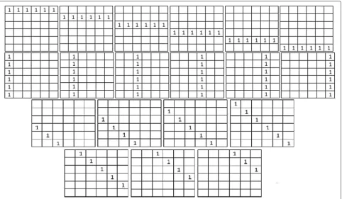
In the training phase, patches are extracted from a num-ber of natural images. These images are taken from the set provided by Yang et al. [11]. These sets of natural images are very rich in high-frequency content and are suitable for the training of dictionaries. To obtain the training set first, the LR counterparts of the HR images are obtained by down-sampling and blurring. These LR images are then interpolated by bicubic interpolation to match the dimensions of the HR images for conve-nience and called those images the mid-resolution (MR) images. Patches are extracted from HR and MR images from the same spatial locations and classified into nine clusters. The patch templates for clustering are designed with the eight different directional orientations to cover the two-dimensional image space and are given asy = {0◦, 22.5◦, 45◦, 67.5◦, 90◦, 112.5◦, 135◦, 157.5◦}. Each clus-ter template created has a specific direction with all pos-sible shifts. These directional orientations given inywere selected after performing various tests and experiments for the optimum performance. The current directional spacing between the templates is 22.5◦. If this value was increased, the number of clusters will be less and so will be the performance of the algorithm. On the con-trary, if this value was less the number of clusters will increase thereby increasing the computation cost at the image recovery stage. Some of the directional templates are shown in Fig. 3 along with their shifted versions. For all the eight directions, we have considered all possible shifts.

Fig. 3Samples of some directional templates showing 0◦, 90◦, and 45◦orientations

on different patch sizes and number of samples of train-ing data, the threshold value 0.69 was selected for the optimum performance of the algorithm. Next, a coupled dictionary learning problem is formulated and solved to obtain the clustered dictionary pairs and their mapping functions.

LetW_Hy andW_Lybe the HR and LR training data, respec-tively. The following energy function is proposed and minimized (approximately); by solving, the corresponding compact directional dictionaries along with the needed mapping function are obtained [13].

min{Dy_H,Dy_L,f(·)}Edata(DyH,W y

H)+Edata(DyL,W y L) +γEmap(f(α_Hy),α_Ly)+λEreg(α_Hy,α_Ly,f(·),Dy_H,Dy_L),

(5)

where Edata(·,·)is the data fidelity term,Emap(·,·) is the mapping fidelity, andEregis the regularizer. The coupling between the sparse coefficients of HR and LR data over dictionaries is related by the mapping functionf(·). The HR and LR dictionaries are optimized concurrently with the mapping function.

The problem in Eq. 5 can be converted into a ridge regression and dictionary learning problem considering the mapping to be a linear function as:

min{Dy_H,Dy_L,f(·)}W_Hy −D_Hyαy_H2_F+ W_Ly−Dy_Lαy_L2_F +γαy

L−Myα y H2F+λ

y Hα

y

H1+λyLα y

L1+λymMy2F s.t.Dy_H,il2 ≤1∧ D

y

L,il2 ≤1 , for alli,

(6)

where γ,λy_H,λym, and λyL represent the regularization

terms for the optimum performance, andDy_H,iandDy_L,iare the atoms ofDy_HandDy_L, respectively.

The problem formulated by Eq. (6) can be solved by optimizing one parameter at a time while considering the others as being constant. As the mapping function (matrix)Myis linear, bi-directional transforms are learned fromα_Hy toαy_Land vice versa.

After initializing matrixM and dictionaryD, one can find the sparse coefficientsαby applying:

min{αy_H}W_Hy −Dy_Hαy_H2_F+γα_Ly−My_Hα_Hy_F2+λy_Hα_Hy1

min{α_Ly}W_Ly−D_Lyα_Ly2_F+γα_Hy −M_Lyα_Ly2_F+λy_Lαy_L1. (7)

The problem in Eq. 7 can easily be solved by apply-ing l1norm minimization algorithm such as least-angle regression (LARS) [14].

min{Dy_H,Dy_L}W_Hy −Dy_Hαy_H2_F+ W_Ly−Dy_Lα_Ly2_F s.t. for alli,D_Hy_,il2 ≤1∧ D

y

L,il2 ≤1. (8)

Now the problem in Eq. 8 is calledquadratically con-strained quadratic program (QCQP). It can be easily solved as done in [11]. Finally by keeping the dictionary and the sparse coefficients fixed, the matrix M can be updated as:

min{My}αy_L−Myα_Hy2_F+(λym/γ )My2_F. (9)

The problem in Eq. 9 is called the ridge regression problem and can be solved as:

My=αy_L(α_Hy)T(α_Hy(α_Hy)T +(λym/γ )·I)−1, (10)

where I represents the identity matrix. By this strategy, a set of directional dictionaries is developed along with their mapping function (matrix). The proposed training algorithm is summarized in Algorithm 1.

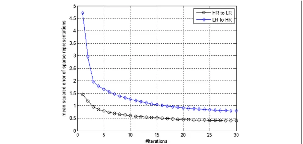
Figure 4 shows the convergence curves of the proposed algorithm. Here mean squared error is calculated from HR to LR and then LR to HR sparse representations of the training patch pairs after updating the HR and LR map-ping matrices in each iteration. The mapmap-ping functions are initialized as the identity matrices and our proposed algorithm converges stably.

3.2 The proposed image reconstruction algorithm During the reconstruction stage, a set of test images is selected from different datasets [15, 16], and also, some benchmark images are selected for testing proposed algo-rithm. Figure 5 shows the images used in the testing phase.

Care has been taken in selecting the images. It was made sure to take the images different from the training set. At the image recovery stage, a given LR image is first up-converted into the MR level by bicubic interpolation. This is done for matching the size of the HR and the (now transformed) LR image. Patches and features are extracted from this up-converted image by applying a full overlap selection scheme. This is followed by a selective sparse coding step. It needs to be identified which dictionary pair along with its mapping function gives the least sparse representation error.

This corresponds to a model selection scenario. We need to find which dictionary pair among the nine clusters will give the least sparse representation error and hence the best HR patch recovery. This is done by recovering HR patch from LR patch at hand using each directional dictionary pair and its mapping function. For patch-based sparse recovery, first the sparse coefficients of the LR patch are calculated by [14] using the LR patch and LR dictionary. Then HR dictionary is used along with map-ping functions to recover the HR patch assuming the invariance property of the sparse coefficients. The dic-tionary and mapping pair which gives the least sparse representation error is chosen for the HR patch estima-tion. Here a very basic approach is presented to show the need and effect of directional clustering. By using all dictionaries for HR, patch recovery serves as a per-fect model selection (PMS) which can be used as a ref-erence while designing different cluster selection mod-els. In this case, the results show peak signal to noise ratio (PSNR) improvements of 1 dB over the baseline algorithms.

Fig. 5Images used in testing phase. Fromlefttorightandtoptobottomcorrespond toAnnieYukiTim,Barbara,BooksCIMAT,Butterfly,Fence,

ForbiddenCity,HowMany,Kodak-05,Kodak-08,Michoacan,MissionBay,NuRegions,Peppers,Rocio,Starfish,Yan

Finally, those approximated HR vector patches are reshaped into two-dimensional form. As we know, patches were extracted with full-overlap, and the overlap-add method of [11] is employed at the end to get the approx-imate HR image. The reconstruction process is summa-rized in Algorithm 2.

4 Results and discussion

The proposed algorithm is compared with the algorithm of Yang et al. [11], algorithm of Xu et al. [12], and Bicubic technique (Bic.).

Tables 1 and 2 list the PSNR, structural similarity index measurement (SSIM) [17], Sharpness and contrast [18] measures for the compared algorithms on different scale parameters. Table 1 shows the results for scale parameter 2. Table 2 shows the results for scale parameters 3 and 4. The proposed algorithm uses a patch size of 6×6 with 216 dictionary atoms for each directional cluster. The base-line algorithm of Yang et al. [11] and the algorithm of Xu et al. [12] use a patch size of 6×6 with 216 dictionary atoms in the spatial domain. The algorithms being com-pared are of different nature and care has been taken to use the values that give optimum performance of the algo-rithms, being compared. Full overlapping is employed for all the algorithm to achieve the best performance. A sin-gle data set of training images used by [11] is selected here for patch extraction and around 10,000 patches were extracted for each cluster for the proposed algorithm and around 100,000 patches were extracted for the spatial domain algorithm of Yang et al. [11] and Xu et al. [12]. The simulation was carried out by setting all other param-eters same. Images for all algorithms are super-resolved by different scale parameters. For the implementation of the Bicubic technique Matlab’s (imresize) function is used. The baseline algorithm of Yang et al. [11] uses a single uni-versal dictionary for the task of SISR as well as [12] does. The proposed algorithm uses nine compact dictionaries covering eight different orientations of the image feature space.

4.1 Quantitative experimentation

LR images are reconstructed by the three algorithms and bicubic technique to their original sizes. The PSNR and SSIM as given in [11] and [17] are used along with sharp-ness and contrast measures used by Liu et al. [18] for the quantitative performance evaluation.

The PSNR measure for a reconstructed image is calcu-lated as follows:

MPSNR(x,xˆ)=10 log10 2552 EMSE(x,xˆ)

, (11)

wherexis the original HR image having size ofM×N,xˆ

is the estimation, andEMSE(x,xˆ)is the mean square error (MSE) given forxandxˆas follows:

EMSE(x,xˆ)= 1 MN

M

i=1 N

j=1

(xij− ˆxij)2. (12)

The SSIM [17] is used as a perceptual quality met-ric, which is more compatible with human image quality perception than the PSNR measure. The sharpness and contrast measures, as introduced by Liu et al. [18], are at first calculated as s(i,j) and c(i,j), respectively, for each pixel position(i,j)and then averaged for the whole image. Regarding s(i,j) and c(i,j), consider an image I and A(i,j) as being the 8-adjacent pixels “around” (i,j) (not including(i,j)); then

s(i,j)= I(i,j)−μA(i,j)1 (13)

wheres(i,j)is the sharpness value of imageIat(i,j), and

μA(i,j)the mean value ofIat pixel locations inA(i,j). For the contrast, let

c(i,j)= 1 MN

M

x=1 N

y=1

I(i,j)−I(x,y)1, (14)

Table 1PSNR (top left), sharpness (top right), SSIM (bottom left) and contrast (bottom right), scale factor 2 comparison of the bicubic (Bic.) technique, algorithm of Yang et al.’s [11], algorithm of Xu et al.’s [12] and proposed algorithm

Images Bic. [11] [12] Proposed(PMS) Proposed

AnnieYukiTim 31.42 0.5709 32.79 0.3824 32.76 0.3848 33.83 0.3659 32.86 0.3789

0.9064 0.3280 0.9375 0.1879 0.9376 0.1865 0.9338 0.2038 0.9221 0.1961

Barbara 25.34 0.7400 25.34 0.5531 25.81 0.5555 26.46 0.5439 25.91 0.5438

0.7929 0.5890 0.8356 0.4199 0.8330 0.4207 0.8563 0.4274 0.8360 0.4249

BooksCIMAT 24.89 0.6176 26.02 0.3940 27.17 0.4075 26.62 0.3916 26.21 0.3987

0.8271 0.4075 0.8826 0.2047 0.9039 0.2176 0.8941 0.2272 0.8829 0.2151

Butterfly 27.45 0.4541 30.07 0.2174 29.85 0.2182 31.77 0.1961 30.53 0.1965

0.8984 0.1633 0.9445 0.0145 0.9430 0.0101 0.9508 0.0569 0.9460 0.0356

Fence 25.04 0.6432 26.32 0.4563 27.85 0.4693 27.31 0.4414 26.36 0.4483

0.7448 0.5281 0.8158 0.3271 0.8496 0.3395 0.8332 0.3379 0.8210 0.3289

ForbiddenCity 24.06 0.7143 24.66 0.5559 25.90 0.5718 25.58 0.5465 24.75 0.5569

0.6767 0.5759 0.7549 0.3974 0.7925 0.4078 0.7930 0.4062 0.7899 0.4062

HowMany 27.98 0.5739 29.19 0.3735 29.16 0.3750 30.04 0.3586 29.17 0.3599

0.8686 0.3038 0.9126 0.1571 0.9120 0.1545 0.9000 0.1708 0.8843 0.1637

Kodak-05 23.97 0.7055 24.78 0.5372 25.89 0.5483 25.60 0.5256 25.56 0.5256

0.7235 0.5015 0.7898 0.3365 0.8239 0.3444 0.8154 0.3510 0.8101 0.3449

Kodak-08 22.12 0.7182 22.81 0.5638 23.48 0.5723 23.83 0.5461 22.90 0.5539

0.6995 0.5183 0.7672 0.3569 0.7950 0.3592 0.8027 0.3633 0.7570 0.3602

Michoacan 22.19 0.6614 23.85 0.4851 24.96 0.4992 24.76 0.4702 24.32 0.4729

0.7877 0.4506 0.8388 0.2879 0.8627 0.2979 0.8508 0.3000 0.8346 0.2943

MissionBay 26.67 0.6174 27.90 0.4294 27.86 0.4295 29.27 0.4003 28.89 0.4092

0.8459 0.3475 0.8883 0.1928 0.8868 0.1899 0.9040 0.2129 0.9010 0.2047

NuRegions 19.81 0.5326 21.30 0.3413 22.09 0.3536 22.14 0.3255 21.35 0.3266

0.8469 0.2749 0.9047 0.0780 0.9182 0.0875 0.9207 0.0898 0.9046 0.0848

Peppers 29.95 0.5459 31.22 0.3545 31.94 0.3781 31.91 0.3253 31.56 0.3261

0.9045 0.2395 0.9422 0.1113 0.9583 0.1270 0.9608 0.1382 0.9596 0.1248

Rocio 36.63 0.4019 39.19 0.1816 39.01 0.1821 40.38 0.1516 38.98 0.1674

0.9612 0.1640 0.9778 0.0515 0.9773 0.0455 0.9745 0.0660 0.9799 0.0530

Starfish 30.22 0.5101 32.12 0.2880 32.04 0.2895 33.09 0.2765 32.89 0.2846

0.8923 0.2779 0.9358 0.1239 0.9354 0.1208 0.9365 0.1380 0.9332 0.1331

Yan 26.96 0.6346 28.01 0.4579 27.94 0.4590 29.16 0.4346 28.15 0.4411

0.8276 0.3878 0.8743 0.2268 0.8729 0.2227 0.8795 0.2447 0.8898 0.2357

Average 26.54 0.6026 27.85 0.4107 28.36 0.4184 28.86 0.3937 28.15 0.3994

0.8253 0.3786 0.8752 0.2171 0.8876 0.2207 0.8879 0.2334 0.8783 0.2254

The data in boldface signifies highest value in comparison

with those of the original images. The table shows abso-lute errors (i.e., the absoabso-lute difference in contrast or sharpness from the original value, divided by the origi-nal value). Smaller values indicate less deviation from true contrast and sharpness.

Tables 1 and 2 indicate that images reconstructed by the proposed algorithm have less deviation in terms of sharpness from the original value. This corresponds to the

observation that the proposed algorithm is well able to recover high-frequency components better than the other algorithms. Also, there is slightly more deviation from the original contrast value when compared with the other algorithms.

Table 2PSNR (top left), sharpness (bottom left), SSIM (top right), and contrast (bottom right), for each image first row (scale factor 3) and second row (scale factor 4) comparison of the bicubic (Bic.) technique, algorithm of Yang et al.’s [11], algorithm of Xu et al.’s [12], and the proposed algorithm

Images Bic. [11] [12] Proposed (PMS)

AnnieYukiTim 26.04 0.7870 30.66 0.8957 30.64 0.8950 31.3 0.8990

0.6800 0.3932 0.5118 0.2493 0.5118 0.2463 0.4868 0.2533

26.94 0.7600 27.62 0.8174 27.62 0.8169 28.10 0.8211

0.8059 0.5246 0.6938 0.3900 0.6935 0.3891 0.6719 0.3904

Barbara 24.52 0.7111 25.24 0.7490 24.60 0.7254 25.62 0.7727

0.8606 0.6644 0.7807 0.5842 0.7791 0.5820 0.7629 0.5834

23.60 0.6570 23.82 0.6744 23.82 0.6743 24.15 0.7018

0.9102 0.7360 0.8631 0.6765 0.8628 0.6756 0.8429 0.6732

BooksCIMAT 22.20 0.6360 24.72 0.8102 24.69 0.8087 24.77 0.8210

0.7883 0.5292 0.6059 0.3423 0.6078 0.3417 0.5867 0.3353

21.62 0.5863 22.94 0.7007 22.94 0.7007 23.30 0.7104

0.8585 0.5998 0.7459 0.4505 0.7462 0.4502 0.7310 0.4517

Butterfly 20.99 0.7329 25.89 0.8627 25.83 0.8600 26.65 0.8652

0.6085 0.2283 0.4148 0.0736 0.4119 0.0679 0.3824 0.0876

22.14 0.6990 23.00 0.7564 23.00 0.7550 23.75 0.7655

0.7362 0.3279 0.5921 0.1543 0.5874 0.1520 0.5567 0.1616

Fence 22.20 0.5741 22.70 0.6494 22.69 0.6488 23.84 0.6894

0.8202 0.6847 0.6854 0.5192 0.6793 0.5234 0.6740 0.5378

21.49 0.4885 21.87 0.5547 21.89 0.5545 22.13 0.5692

0.9082 0.7965 0.8420 0.7037 0.8425 0.7033 0.8243 0.7014

ForbiddenCity 22.38 0.4415 24.02 0.6123 24.06 0.6140 24.20 0.6294

0.8500 0.7079 0.7470 0.5722 0.7482 0.5717 0.7185 0.5572

22.06 0.3498 22.73 0.4615 22.74 0.4625 23.23 0.4976

0.9151 0.7982 0.8411 0.6791 0.8426 0.6794 0.8204 0.6733

HowMany 23.56 0.6774 27.15 0.8396 27.12 0.8384 27.71 0.8432

0.6947 0.3788 0.5326 0.2429 0.5338 0.2413 0.5068 0.2460

22.96 0.6048 24.85 0.7303 24.85 0.7295 25.30 0.7995

0.7996 0.4872 0.6855 0.3499 0.6842 0.3493 0.6611 0.3505

Kodak-05 23.05 0.6121 24.28 0.7147 24.25 0.7136 24.81 0.7381

0.8003 0.5698 0.6708 0.4227 0.6716 0.4212 0.6503 0.4251

20.80 0.4341 22.60 0.5945 22.58 0.5936 23.95 0.6320

0.8862 0.6848 0.8120 0.5702 0.8114 0.5691 0.7886 0.5623

Kodak-08 20.72 0.5695 21.84 0.6723 21.84 0.6724 22.50 0.7070

0.8180 0.5988 0.7058 0.4691 0.7065 0.4673 0.6818 0.4688

18.70 0.3914 20.61 0.5493 20.60 0.5497 21.71 0.6603

0.8971 0.7025 0.8349 0.6098 0.8357 0.6080 0.8072 0.6035

Michoacan 21.22 0.6522 22.64 0.7446 22.61 0.7429 23.23 0.7605

0.7766 0.5345 0.6365 0.3887 0.6357 0.3870 0.6112 0.3900

18.76 0.4721 20.84 0.6253 20.81 0.6235 21.10 0.6758

0.8715 0.6503 0.7878 0.5359 0.7886 0.5346 0.7630 0.5290

MissionBay 24.13 0.7399 25.52 0.8019 25.50 0.8021 26.35 0.8167

Table 2PSNR (top left), sharpness (bottom left), SSIM (top right), and contrast (bottom right), for each image first row (scale factor 3) and second row (scale factor 4) comparison of the bicubic (Bic.) technique, algorithm of Yang et al.’s [11], algorithm of Xu et al.’s [12], and the proposed algorithm (Continued)

21.77 0.6162 24.05 0.7309 24.06 0.7305 24.93 0.8129

0.8149 0.5062 0.6985 0.3702 0.6980 0.3704 0.6697 0.3707

NuRegions 15.08 0.5079 18.22 0.7765 18.24 0.7765 18.84 0.7840

0.7198 0.4805 0.5369 0.2410 0.5419 0.2402 0.5176 0.2395

13.39 0.2408 15.70 0.5647 15.72 0.5657 16.21 0.6836

0.8503 0.6714 0.7069 0.4420 0.7091 0.4416 0.6907 0.4369

Peppers 24.00 0.7678 28.58 0.9013 28.52 0.8993 28.99 0.9810

0.6997 0.3360 0.5512 0.2168 0.5502 0.2153 0.5100 0.2160

25.34 0.7786 26.63 0.8377 26.56 0.8355 27.30 0.9130

0.7447 0.3731 0.6059 0.2406 0.6061 0.2382 0.5710 0.2425

Rocio 30.27 0.8704 33.77 0.9376 33.70 0.9327 34.42 0.9390

0.5753 0.2492 0.3732 0.1271 0.3739 0.1237 0.3374 0.1335

29.27 0.8407 31.22 0.8926 31.22 0.8917 32.77 0.9010

0.6694 0.3241 0.5114 0.1975 0.5110 0.1964 0.4725 0.1991

Starfish 24.38 0.7056 28.67 0.8643 28.61 0.8625 29.24 0.8720

0.6675 0.3748 0.4815 0.2229 0.4835 0.2220 0.4580 0.2238

25.18 0.6960 25.79 0.7595 25.78 0.7584 26.34 0.8020

0.7960 0.5033 0.6746 0.3647 0.6734 0.3634 0.6517 0.3616

Yan 24.27 0.6847 26.42 0.8061 26.41 0.8057 27.30 0.8121

0.7470 0.4719 0.5922 0.3134 0.5933 0.3123 0.5640 0.3188

22.74 0.6047 24.12 0.6907 24.14 0.6910 25.71 0.7019

0.8496 0.5864 0.7534 0.4532 0.7527 0.4529 0.7246 0.4526

Average 23.06 0.6669 25.65 0.7899 25.58 0.7874 26.24 0.8081

0.7414 0.4781 0.5900 0.3307 0.5902 0.3293 0.5644 0.3330

22.30 0.5763 23.65 0.6838 23.65 0.6833 24.37 0.7280

0.8321 0.5795 0.7281 0.4493 0.7278 0.4483 0.7030 0.4475

The data in boldface signifies highest value in comparison

algorithm produces better results when compared with Yang et al.’s [11], due to the directional clustered dictio-nary learning. The proposed algorithm gives an average PSNR raise of 1.01, 0.59, and 0.72 dB for scale parame-ters 2, 3, and 4 over the state of the algorithm of Yang et al. [11] with SSIM improvement of 0.0127, 0.0182, and 0.0442 for scale parameters 2, 3, and 4 when tested on [15, 16] data sets and some other benchmark images. The improvements over the coupled K-SVD algorithm of Xu et al. [12] is 0.5, 0.66, and 0.72 dB in terms of PSNR for scale parameters 2, 3, and 4. The improvements in SSIM values are 0.0002, 0.0207, and 0.0447 for scale parameters 2, 3, and 4. The improvements over the bicubic technique over this set of test images is 2.32, 3.18, and 2.07 dB in terms of PSNR for scale parameters 2, 3, and 4 and 0.0623, 0.1412, and 0.1017 in terms of SSIM for scale parameters 2, 3, and 4, respectively. This justifies the fact that direc-tional clustered dictionaries better recover some of the high-frequency components of the LR image.

From Table 1, one can see that the average PSNR and SSIM results of the proposed algorithm are less than the algorithm of [12] for scale parameter 2. This is due to the fact that the algorithm by [12] uses a coupled K-SVD approach for the dictionary update stage, also after recovering the HR patches a geometric mean algorithm is implemented to get the HR image estimate which serves as an additional post processing. However, the proposed (PMS) clearly outperforms the compared algorithms for all scale parameters.

Table 3PSNR (top) and SSIM (bottom), comparison of the bicubic (Bic.) technique, algorithm of Yang et al.’s [11], algorithm of Xu et al.’s [12], and the proposed algorithm

Images Bic. [11] [12] Proposed

Baboon 24.66 25.28 25.30 26.05

0.6359 0.7594 0.7602 0.7746

Boat 32.35 33.71 33.66 35.03

0.8989 0.9292 0.9291 0.9375

Bridge 26.49 27.46 27.46 28.36

0.7922 0.8445 0.8446 0.8725

Cameraman 26.32 27.63 27.61 28.73

0.8629 0.8918 0.8912 0.9132

Coala 33.40 36.26 36.26 37.83

0.8958 0.9513 0.9513 0.9697

Coastguard 29.13 30.47 30.47 31.61

0.7725 0.8495 0.8501 0.8731

Comic 26.05 28.33 28.28 28.78

0.8419 0.9105 0.9092 0.9255

Elaine 31.04 31.31 31.32 31.83

0.6531 0.7123 0.7131 0.7214

Face 34.74 36.53 36.53 36.90

0.8041 0.9095 0.9097 0.9432

Fingerprint 31.92 34.43 34.43 35.14

0.9513 0.9729 0.9730 0.9765

Flowers 30.41 32.19 32.10 33.47

0.8828 0.9270 0.9264 0.9496

Foreman 35.35 37.39 37.20 38.76

0.8928 0.9594 0.9586 0.9686

House 32.76 34.25 34.13 35.72

0.8928 0.9099 0.9092 0.9279

Lena 34.71 36.21 36.18 37.14

0.8507 0.9259 0.9260 0.9737

Man 29.25 30.38 30.33 31.40

0.8314 0.8782 0.8779 0.8905

Parrot 26.91 28.57 28.63 29.75

0.8931 0.9185 0.9186 0.9340

Average 30.34 31.90 31.87 32.91

0.8345 0.8906 0.8905 0.9095

The data in boldface signifies highest value in comparison

It is noted here that the computational cost of the pro-posed algorithm increases nine times as compared to the algorithms of [11] and [12]. It is well known that the most expensive stage in the dictionary learning pro-cess is the sparse representation stage which is a vector selection process. Using each directional dictionary along with mapping to recover the HR patch increases the

computational cost given that the proposed algorithm is using the same number of dictionary atoms and patch size. However, in some applications, one can compromise the number of computations given that the improvement margin in quality is considerable.

We also tested other dictionary model selection approaches which can reduce the computational cost. One approach that we used during the testing phase of the proposed algorithm for cluster selection was only the cor-relation of the LR patch at hand with each directional cluster and then using that dictionary pair for HR patch reconstruction. Using this very simple approach on aver-age using the same test imaver-ages and scale parameter 2, the PSNR improvements were 0.3 dB over the algorithm of [11] and SSIM improvement of 0.0031. These results are given in Table 1 last column. In this case, the computa-tional cost is same as the baseline algorithms with only additional correlation computation. In this scenario, the only extra cost is the correlation computation for cluster decision when comparing with the baseline algorithms. In the same way, one can use different probabilistic models for deciding which cluster to use during the reconstruc-tion phase given that the clustering is carried out by correlation with designed templates. One can also exploit hidden Markov trees (HMT) between the HR and LR training data and develop suitable models.

4.2 Qualitative experimentation

Here, the zoomed versions of the reconstructed images for scale parameter 3 are shown for the comparison. Figure 6 shows the zoomed original image and the recon-structed images by the algorithms used for comparison. Images are zoomed to further clarify the comparisons. Looking into Fig. 6, one can see that the reconstruc-tion by bicubic technique shows a significant amount of blur; however, the reconstructed images by the algo-rithm of Yang et al. [11] are slightly clearer than the bicubic technique. Looking at the zoomed Barbaraand Kodak-05image, it is clear that the reconstruction by the proposed algorithm is much sharper around the edges and more clear in terms of sharpness best viewed on HD device. The proposed algorithm is able to recover the sharper patches more efficiently than the baseline algorithm.

5 Conclusions

Fig. 6Visual comparison ofBarbara,Kodak-05,Starfish,Yan, fromlefttorightcorrespond to: original, bicubic, [11, 12], and proposed method

Xu et al. [12] due to clustering and coupled dictionary learning with mapping functions.

From the results, it can be seen that the proposed idea of clustering-based coupled dictionary learning and map-ping functions can produce better results when compared with the state-of-the-art algorithms.

For scale parameter 2 compared to the bicubic interpo-lation, the proposed algorithm gives 2.32 dB improvement as tested over the set of benchmark images. The proposed algorithm provides a 1.01 dB improvement over the base-line algorithm of Yang et al. [11], and 0.5 dB improvement over the algorithm of Xu et al. [12] as tested over the image data sets [15, 16]. Visual results also verify those quantitative results.

5.1 Future recommendations

Considering the possibilities of the extension of this work, it is suggested that in the process of designing dictionar-ies, one can employ the model selection from LR to HR by learning hidden Markov models [19]. Moreover, to gener-ate the LR images, the blur filter is assumed as the bicubic filter. This work can be extended to include and compare the accurate camera blur models as in [20].

Authors’ contributions

Both the authors have contributed equally to the text, while JA has implemented the algorithms and performed most of the tests. Both authors read and approved the final manuscript.

Competing interests

The authors declare that they have no competing interests.

Received: 18 April 2016 Accepted: 7 October 2016

References

1. M Elad, M Aharon, Image denoising via sparse and redundant representations over learned dictionaries. IEEE Trans. Image Process. (TIP).15, 3736–3745 (2006)

2. DL Donoho, Compressed sensing. IEEE Trans. Inf. Theory.52, 1289–1306 (2006)

3. J Yang, J Wright, T Huang, Y Ma, Image super-resolution via sparse representation. IEEE Trans. Image Process.19(11), 2861–2873 (2010) 4. B Ophir, M Lustig, M Elad, Multiscale dictionary learning using wavelets.

IEEE J. Sel. Topics in Signal Process.5(5), 1014–1024 (2011)

5. K Zhang, X Gao, D Tao, X Li, inProceedings of International Conference on Computer Vision and Pattern Recognition (CVPR’12). Multi-scale dictionary for single image super-resolution (IEEE Providence, RI, USA, 2012), pp. 1114–1121

6. W Dong, L Zhang, G Shi, X Wu, Image deblurring and super-resolution by adaptive sparse doamin selection and adaptive regularization. IEEE Trans. Image Process.20, 1838–1857 (2011)

7. J Feng, L Song, X Yang, W Zhang, inProceedings of the IEEE International Conference on Image Processing, (ICIP’11). Learning dictionaries via subspace segmentation for sparse representation (IEEE Brussels, Belgium, 2011), pp. 1245–1248

8. G Yu, G Sapiro, S Mallat, inPreceedings of IEEE International Conference on Image Processing, (ICIP’10). Image modelling and enhancement via structured sparse model selection (IEEE, Hong Kong, 2010), pp. 1641–1644 9. S Yang, M Wang, Y Chen, Y Sun, Single image super-resolution

reconstruction via learned geometric dictionaries and clustered sparse coding. IEEE Trans. Image Process.21, 4016–4028 (2012)

image super-resolution based on sparse representation via directionally structured dictionaries (IEEE Trabzon, Turkey, 2014), pp. 1718–1721 11. J Yang, Z Wang, Z Lin, S Cohen, T Huang, Coupled dictionary training for

image super-resolution. IEEE Trans. Image Process.21, 3467–3478 (2012) 12. J Xu, C Qi, Z Chang, inProceedings of IEEE International Conference on

Image Processing (ICIP’14). Coupled K-SVD dictionary training for super-resolution (IEEE, Paris, France, 2014), pp. 3910–3914

13. S Wang, L Zhang, Y Liang, Q Pan, inProceedings of International Conference on Computer Vision and Pattern Recognition (CVPR’12). Semi-coupled dictionary learning with applications to image super-resolution and photo-sketch synthesis (IEEE Providence, RI, USA, 2012), pp. 2216–2223 14. B Efron, T Hastie, I Johnstone, R Tibshirani, Least angle regression. Ann.

Stat.32, 407–499 (2004)

15. R Franzen, Kodak lossless true color image suite (2014). onliner0k.us/ graphics/kodak/index.html. accessed 20 January 2016

16. R Klette,Concise computer vision. (Springer, London, 2014). Single images. online:ccv.wordpress.fos.auckland.ac.nz/data/single-images/. accessed 20 Jan 2016

17. Z Wang, AC Bovik, HR Sheikh, EP Simoncelli, Image quality assessment: from error visibility to structural similarity. IEEE Trans. Image Process.

13(4), 600–612 (2004)

18. D Liu, R Klette, inProceedings of International Conference on Image Vision Computing New Zealand (IVCNZ’15). Sharpness and contrast measures on videos (IEEE Auckland, New Zealand, 2015). IEEE online

19. RK Lama, MR Choi, GR Kwon, Image interpolation for high-resolution display based on the complex dual tree wavelet transform and hidden markov. Multimedia Tools Appl. online, 1–12 (2016)

20. N Efrat, D Glasner, A Apartsin, B Nadler, A Levin, inProceedings of IEEE International Conference on Computer Vision (ICCV’13). Accurate blur models vs. image priors in single image super-resolution (IEEE Sydney, Australia, 2013), pp. 2832–2839

Submit your manuscript to a

journal and benefi t from:

7Convenient online submission

7Rigorous peer review

7Immediate publication on acceptance

7Open access: articles freely available online

7High visibility within the fi eld

7Retaining the copyright to your article