R E S E A R C H
Open Access
Sequential Monte Carlo filter based on
multiple strategies for a scene specialization
classifier
Houda Maâmatou
1,2,3*, Thierry Chateau
1, Sami Gazzah
2, Yann Goyat
3and Najoua Essoukri Ben Amara
2Abstract
Transfer learning approaches have shown interesting results by using knowledge from source domains to learn a specialized classifier/detector for a target domain containing unlabeled data or only a few labeled samples. In this paper, we present a new transductive transfer learning framework based on a sequential Monte Carlo filter to specialize a generic classifier towards a specific scene. The proposed framework utilizes different strategies and approximates iteratively the hidden target distribution as a set of samples in order to learn a specialized classifier. These training samples are selected from both source and target domains according to their weight importance, which indicates that they belong to the target distribution. The resulting classifier is applied to pedestrian and car detection on several challenging traffic scenes. The experiments have demonstrated that our solution improves and outperforms several state of the art’s specialization algorithms on public datasets.
Keywords: Generic and specialized classifier, Sequential Monte Carlo filter, Sample-proposal and observation strategies, Specialization, Transductive transfer learning
1 Introduction
The object detection in an image or in video frames is the first task to perform and the most interesting one in several computer vision applications. A lot of work has focused on pedestrian and vehicle detection for the intel-ligent development of the transportation system and the video-surveillance traffic-scene analysis [1–13]. Most of these papers have proposed object-appearance detectors to improve the performance of the detection task and to avoid—or at least reduce—problems relative to a simple background subtraction algorithm, such as merging and splitting blobs, detecting mobile background objects, and detecting moving shadows. Some researchers [9, 10, 14] have focused on presenting relevant features that drop the false positive rate and raise the detection accuracy, though often leading to a increase in the computational costs of multi-scale detection tasks. Other researchers, like Dollár et al. [11, 12], have been interested in reducing
*Correspondence: [email protected] 1Institut Pascal, Blaise Pascal University, 24 Avenue des Landais, Clermont-Ferrand, France
2SAGE ENISo, University of Sousse, BP 264 Sousse Erriadh, Sousse, Tunisia Full list of author information is available at the end of the article
the time needed to compute features at each scale of sampled image pyramids without adding complexity or particular hardware requirements to allow fast multi-scale detection.
However, a key point of learning appearance-based detectors is the building of a training dataset, where thou-sands of manual labeled samples are needed. This dataset should cover a large variety of scales, view points, light conditions, and image resolutions. In addition, training a single object detector to deal with various urban scenarios is a very hard task because there can be much variabil-ity in traffic scenes like several object categories, different road infrastructures, weather influence on video quality, and time of scene recording (rush hours or off-peak hours, day or night).
The diversity of both positive and negative samples can be very restricted in a video surveillance scene recorded by one static camera. Nevertheless, it was demonstrated in [15–20] that the accuracy of a generic (pedestrian or vehi-cle) detector would drop-off quickly when it was applied to a specific traffic scene, in which the available data would mismatch the training source one.
An intuitive solution is to build a scene-specialized detector that provides a higher performance than a generic detector using labeled samples from the target scene. On the other hand, labeling data manually for each scene and repeating the training process several times, according to the number of object classes in the target scene, are arduous and time-consuming tasks. A functional solution to keep away from these tasks is to automatically label samples from the target scene and to transfer only a set of useful samples from the labeled source dataset to the target specialized one. Our work moves along this direction. We suggest an original formal-ization of transductive transfer learning (TTL) based on a sequential Monte Carlo (SMC) filter [21] to specialize a generic classifier to a target scene. In the proposed for-malization, we estimate a hidden target distribution using a source distribution in which we have a set of annotated samples, in order to give an estimated target distribu-tion as an output. We consider samples of the training dataset as realizations of the joint probability distribution between samples’ features and object classes.
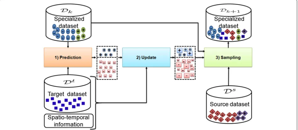
The distribution approximation is solved by a recursive process. A synthetic block diagram corresponding to one iteration is illustrated in Fig. 1. Algorithm 1 describes the process of the suggested approach. In this algorithm, we start with a prediction step that applies sample-proposal strategies on a set of frames extracted from the target scene to search and suggest target samples. Then, we determine the relevance of the proposals in the update step using observation strategies that assign a weight to each proposal sample. The sampling step uses a sampling importance resampling (SIR) algorithm to select target
samples with a high weight and to pick out source sam-ples that are visually close to the selected target ones. The selected samples from both the target and source datasets are combined to create a new specialized dataset for the next iteration. When the stopping criterion is reached, we provide the last specialized classifier and the associated specialized dataset as outputs.
Our major contribution in this paper concerns the use of the Monte Carlo filter in a context of transfer learning:
(1) Original formalization of TTL for classifier spe-cialization based on SMC filter:This formalization is inspired from particle filters, mostly used to solve the problems of object tracking and robot localization [22–24]. We propose to approximate an unknown target distribution as a set of samples that compose the specialized dataset. The aim of our formalization is to automatically label the target data, to attribute weights to samples of both source and target datasets reflecting their relevance, to select relevant samples for the training according to their weights, and to train a scene specialized classifier. Importantly, this formalization is general and can be applied to special-ize any classifier.
Moreover, we propose different strategies for the three steps of the Monte Carlo filter:
(2) Strategies of sample proposal: In order to use infor-mative samples for training a scene-specialized clas-sifier, we put forward two sample-proposal strategies. The letter gives a set of suggestions composed by true
positive samples, false positive ones known as “hard examples,” and samples from background models. These strategies accelerate the specialization process by avoiding handling all the samples of the target database.
(3) Strategies of observation: We also suggest two obser-vation strategies to select the correct proposed target samples and to avoid the distortion of the special-ized dataset with mislabeled samples. These strategies utilize prior information, extracted from the target video sequence, and visual context cues to assign a weight for each sample returned by the proposal strategies. Our suggested visual cues do not incorpo-rate the score returned by the classifier, which can make the training of the specialized classifier drift, as some previous work did [25–28].
(4) Strategy of sampling: In general, the properly classi-fied target samples are not enough to build an effi-cient target classifier. However, the source dataset may contain some samples that are close to the target ones, which helps training a specialized clas-sifier. Therefore, we put forward a sampling strat-egy that selects useful samples from both target and source datasets according to their weight impor-tance, reflecting the likelihood that they belong to the target distribution. Differently from the work devel-oped in [25–28], which treated equally the dataset samples, or from the work of Wang et al. [16, 17], which integrated the confidence-score associated to the sample in the training function of the classifier, we utilize the SIR algorithm. The latter transforms the weight of a sample on a number of repetitions, through replacing the samples associated to a high weight by numerous ones and replacing the sam-ples linked to a low weight by few ones, thus giving them identical weights. This makes our approach applicable to specialize any classifier, while treating training samples according to the importance of their weights without modifying the training function as Wang et al. [16, 17] did.
The remainder of the paper is organized as follows. First, some related work is described in Section 2. Then, the proposed approach is presented in Section 3: We describe the general SMC scene specialization framework in Section 3.1 and the several proposed strategies for each filter step in Section 3.2. After that, our experimen-tal results are provided in Section 4. Finally, the paper is summarized in Section 5.
2 Related work
The literature has proven that the transfer learning meth-ods have been successfully utilized in various real-world applications like object recognition and classification.
These methods propose to use available annotated data and knowledge acquired through some previous tasks rel-ative to source domains so as to improve a learning system of a target task in a target domain [29]. In this section, we are interested in the work that suggests to develop auto-matically or with less human effort-specific classifiers or detectors to a target scene.
Mainly three categories of transfer learning methods, related to the suggested approach, were described in [20]. The first category would modify the parameters of a source learning model to improve its accuracy in a target domain [30, 31]. The second one would reduce the differ-ence between the source and target distributions to adapt the classifier to the target domain [32, 33]. The last one would automatically select the training samples that could give a better model for the target task [34, 35]. Except [18, 36], which presented classifiers based on the Convo-lutional Neural Networks (CNN), most of the work cited above was presented as variants of the Support Vector Machine (SVM).
Futhermore, some solutions concatenated the source dataset with new samples, which increased the dataset size during iterations [30–33]. Others were limited only to the use of samples extracted from the target domain [28], which resulted in losing pertinent information of source samples. Ali et al. [37] presented an approach that learned a specific model by propagating a sparsely labeled training video based on object tracking. Inspired from this, Mao and Yin [19] opted for chains of tracked samples (track-lets) to automatically label target data. They linked detec-tion samples returned by an appearance-object detector into tracklets and propagated labels to uncertain tracklets based on a comparison between their features and those of labeled tracklets. The method used a lot of parameters, which should be determined or estimated empirically, and several sequential thresholding rules, causing an ineffi-cient adaptation of a scene-specific detector.
Another solution was proposed in [15–18, 20, 35, 36]. It collected new samples from the target domain and selected only the useful ones from the source dataset. Wang et al. [17] used different contextual cues such as pedestrian motion, road model (pedestrians, cars ...), loca-tion, size, and objects’ visual appearances to select positive and negative samples of the target domain. In fact, their method was based on a new SVM variant to select only source samples that were good for the classification in the target scene. The limit of their method was that it can be applied only onto an SVM classifier.
Recently, we have noticed an emergence of work based on deep learning, which presents high performances on classification and detection tasks. Yet, it is known that this type of model requires large datasets and has various parameters to train. In order to take advantage of these classifiers, some work has proposed to transfer the CNN trained on a large source dataset to a target domain with a small dataset. Oquab et al. [38] copied the weight from a CNN trained on the ImageNet dataset to a target net-work with additional layers for image classification on the Pascal VOC dataset. In [18], Li et al. suggested adapt-ing a generic ConvNet vehicle detector to a scene-specific one by reserving shared filters between source and tar-get data and updating the non-shared filters. In contrary with [18, 38], which needed several labeled data in the tar-get domain, Zeng et al. [36] learnt the distribution of the target domain by opting for Wang’s approach [17] as an input to their deep model to re-weight samples from both domains without manual data labeling from the target scene.
Most of the specialization algorithms cited above are based on hard-thresholding rules and can drift quickly during training [17], or they are applied only to few classifiers. Nevertheless, our proposed framework over-comes the risk of drifting by propagating a subset of specialized dataset through iterations. It can be used to
specialize any classifier while utilizing the same function as a generic classifier and may be applied using several strategies on each step of the filter. Some preliminary results of the work presented in this paper were published in [20]. In this paper, we put forward an extension of our original TTL approach based on an SMC (TTL-SMC) filter by other sample proposal and observation strate-gies and more experiments. The TTL-SMC approximates iteratively the joint probability distribution between the samples and the object classes of the target scene by com-bining only relevant source and target data as a specialized dataset. The latter is used to train a specialized classifier for the target scene.
3 Our proposed approach
This section presents the proposed approach. We describe in Section 3.1 the core of the general specialization frame-work based on the SMC filter. Then, we suggest in Section 3.2 different strategies that can be used for each filter step.
3.1 SMC scene specialization framework
This subsection introduces the context and gives a detailed description of the proposed framework.
3.1.1 Context
In our work, we assume that the unknown joint distribu-tion between the target samples and the associated labels can be approximated by a set of representative samples. The block diagram of the suggested specialization, at a given iterationk, is illustrated in Fig. 1. Algorithm 1 gives a summary of its process.
Given a source dataset, a generic classifier, which can be learnt from this source dataset, and a video sequence of a target scene, then a specialized classifier and an associated specialized dataset are to be generated. The two latter are the outputs of the distribution approximation provided by the SMC filter.
LetDk = {. X(kn)}n=1,..,N be a specialized dataset of size N at an iterationk, whereX(kn) =. (x(n),y)is the sample numbern, withxbeing its feature vector andyits label, wherey∈ Y. Basically,Y = {−1; 1}, where 1 represents
the object and −1 represents the background (or non-object class). In addition,Dk is a specialized classifier at
an iterationk, which is trained on the previous specialized datasetDk−1. We use a generic classifier g at the first
iteration.
A source datasetDs= {. Xs(n)}
n=1,..,NsofNslabeled
Algorithm 1SMC scene specialization algorithm
Input: Source datasetDs
Generic classifierg
Target video scene and associated datasetDt Number of source samplesNs.
Parameterαs.
Output: Last specialized datasetD Last classifierD
________________________________________
k←0
stop←false
while stop=truedo
/* Prediction step */
if(Dk =∅)then Learn(g,Ds)∗ else
Learn(Dk,Dk)∗ end if
˜ Dk+1←
˜
X(kn+)1
n=1,..,N˜k+1
if(| ˜Dk+1|/| ˜Dk|>=αs)then stop←true
Break end if
/* Update step */ ˘
Dk+1←
˘
Xk(n+)1,π˘k(n+)1
n=1,..,N˘k+1
/* Sampling step */ Dk+1←
X∗k(+n1)
n=1,..,Ns k←k+1
end while
∗Learn(,D)is a function that learns a classifieron
the datasetD.
3.1.2 Classifier specialization based on SMC filter
We define Xk as a hidden random state vector
associ-ated to a joint distribution between features and labels of dataset samples at an iterationkandZka random measure
vector associated to information extracted from the tar-get video sequence. Based on our assumption, fixed above, the target distribution can be approximated iteratively by applying Eq. 1:
pXk+1|Z0:k+1
=
C.pZk+1|Xk+1
Xk
pXk+1|Xk
p(Xk|Z0:k)dXk
(1)
withC=1/p(Zk+1|Z0:k+1).
The SMC filter approximates the posterior distribution
p(Xk|Zk) by a set ofN particles (samples in this case),
according to Eq. 2:
p(Xk|Zk)≈
1
N N
n=1 δX(kn)
≈X(kn)
n=1,..,N (2)
Therefore, the SMC filter is used to estimate the unknown joint distribution between the features of the target samples and the associated class labels by a set of samples that are initially unknown. We suppose that the recursion process selects relevant samples for the spe-cialized dataset from one iteration to another, leads to converge to the right target distribution, and makes the resulting classifiers more and more efficient.
The resolution of Eq. 1 is done in three steps: prediction, update, and sampling. The following paragraphs describe the details of each one.
Prediction step: The prediction step consists in applying the Chapman-Kolmogorov (Eq. 3):
pXk+1|Z0:k
=
Xk
pXk+1|Xk
p(Xk|Z0:k)dXk (3)
Equation 3 uses the term p(Xk+1|Xk) of the system
dynamics between two iterations in order to propose a specialized dataset Dk =.
X(kn)
n=1,..,Ns producing the
approximation (4):
pXk+1|Z0:k
≈X˜(kn+)1
n=1,..,N˜k+1
(4)
We note D˜k+1 =.
˜
X(kn+)1
n=1,..,N˜k+1
the specialized
dataset predicted for an iteration(k+1)whereN˜k+1is its
number of samples andX˜(kn+)1is thenthpredicted sample. Update step: This step defines the likelihood term (5) by using a set of observation strategies. These latter help to assign a weightπ˘k(n+)1to each sampleX˘(kn+)1returned by the classifier at the prediction step.
pZk+1|Xk+1= ˘X(kn+)1
∝ ˘π(n)
k+1 (5)
The observation strategies employ visual contextual cues and prior information extracted from the target video sequence, like object motion, a KLT feature tracker, a background subtraction algorithm, and/or an object path model, to favor a proposition with a correct label. These observation strategies are detailed in Section 3.2.2. The output of this step is a set of weighted target samples, which will be referred to as “the weighted target dataset,” hereafter (6):
˘
X(kn+)1,π˘k(n+)1
n=1,..,N˘k+1
where (X˘(kn+)1,π˘k(n+)1) represents a target sample with its associated weight and N˘k+1 is the number of weighted
samples.
Sampling step: The goal of this step is to build a new specialized dataset by deciding, according to a sampling strategy, which samples will be included in the produced dataset. This latter approximates the posterior distribu-tionp(Xk+1|Z0:k+1)according to (7):
pXk+1|Z0:k+1
≈X∗k(+n1)
n=1,..,Ns (7)
X∗k+(n1)is a selected samplento be in the next specialized dataset Dk+1; a sample can be selected either from the target dataset or from the source one.
It is to note that in this step we apply the SIR algorithm to approximate the conditional distributionp(X˘k+1|Zk+1)
of the target samples given by the observations. Further-more, we propose to extend this target set by transferring samples from the source dataset, which mostly resemble those of the target scene, without changing the posterior distribution.
The specialization process stops when the ratio
(| ˜Dk+1|/| ˜Dk|)exceeds a previously fixed thresholdαs.| • |
represents the dataset cardinality. The output classifier will be based only on appearance to detect the interest object (pedestrian or car) on the target scene.
3.2 The different proposed strategies
In this subsection, we propose several strategies in each filter’s step. This filter aims to specialize a classifier to a target scene surveilled by a static camera.
In the description below, we consider a pedestrian as our interest object, but the strategies can be applied for any other objects, e.g., cars and motorbikes.
3.2.1 Sample proposal strategies
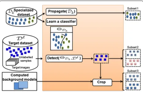
The sample proposal strategies consist in suggesting a set of target samples to be added in the specialized dataset.
Fig. 2Processing details of sample proposal strategies
Figure 2 shows an overview of the processing at a given iteration.
In our case, the proposal dataset is composed of three subsets:
• Subset 1: It corresponds to sub-sampling the spe-cialized dataset resulting from the previous iteration to propagate the distribution from one iteration to another. The ratio between the positive and negative classes (typically the same as the one of the source dataset) should be respected. This subset approxi-mates the termp(Xk|Z0:k)in Eq. 1, according to Eq. 8:
p(Xk|Z0:k)≈
X∗k(+n1)
n=1,..,N∗ (8)
whereX∗k(+n1) is the sample n selected fromDk to be in the dataset of the next iteration(k+1)andN∗is the number of samples in this subset withN∗=αtNs, where αt ∈[ 0, 1]. The parameterαt determines the number of samples to be propagated from the previous dataset.
• Subset 2: To get this subset, we train a new specialized classifierθDk onDk and use it to detect a pedestrian on a set of frames extracted uniformly from the target video-sequence, using a multi-scale sliding window technique. This technique covers a pedestrian by sev-eral bounding boxes, so a spatial mean-shift grouping function is opted for to merge the closest bounding boxes. Moreover, it provides a set of samples classified as a pedestrian, but there are true and false detections. Herein, we suppose that each detection can be either a positive sample or a negative one. Thus, each detec-tion is duplicated: one sample is labeled positively and the other one is labeled negatively. This subset is returned by Eq. 9:
˘
X(kn+)1 n=1,..,N˘k
. =
x(n),y
y∈Y;x(n)∈Dt/ Dk(x(
n))>0
(9)
˘
X(kn+)1is thenthtarget sample proposed to be included in the dataset of the next iteration(k+1).
• Subset 3: In some cases, the previous specialized clas-sifier would rather miss detections than give false positive ones; and it is difficult to favor a label for sev-eral samples in subset 2. This means that we cannot select enough negative target samples to specialize the classifier from subset 2.
according to Eq. 10.
˘
Xk(+n)1
n=1,..,M˘k
. =
∪
bjin{b1,...,bm}
(x(n),−1)
x(n)∈bj
(10)
where (x(n),−1) is a sample cropped from a target background model and labeled negatively.M˘k =m∗
˘
Nkis the number of all background samples.
We crop a sample from each computed background model, at the same position and with the same size of each selected sample returned by the classifier.
Figure 3 shows an illustration of the proposal strategy to crop samples of subsets 2 and 3 from a target frame. At the first iteration, subset 1 is empty and the proposals composing subsets 2 and 3 are given by using a generic detector trained on the INRIA person dataset, in a similar way to the one proposed by Dalal and Triggs in [9].
3.2.2 Observation strategies
As depicted in Fig. 3, some target samples are misclas-sified, which are known as “hard examples.” It is unre-liable to directly use these samples according to their predicted labels or not to utilize them in the specializa-tion process because they are probably informative. In what follows, we present several strategies of the weight-ing samples of subset 2 in order to choose the correct
Table 1Functions and notations used in Algorithm 2
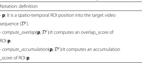
Notation: definition
-p: It is a spatio-temporal ROI position into the target video
sequence (Dt).
-compute_overlap(p,Dt):It computes an overlap_score of
ROIp.
-compute_accumulation(p,Dt):It computes an accumulation
_score of ROIp.
proposal using the information extracted from the target scene.
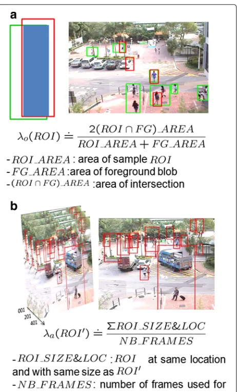
1 - Overlap accumulation scores: Our first strategy, called overlap accumulation scores (OAS), is based on two simple spatio-temporal cues: a background extraction overlap score and a temporal accumulation one.
In a traffic scene, it is rare for pedestrians to stay stable for a long time, and a good detection occurs on a foreground blob; whereas, false positive background detections provide some region of interests (ROIs) that appear over time at the same location and with almost the same size.
Considering this, favoring automatically the sample associated to the right label becomes easier and is done by applying Algorithm 2. Table 1 outlines some notations used in Algorithm 2.
Algorithm 2Observation strategy 1: OAS
Input: Subset 2
˘ X(kn+)1
n=1,..,N˘ with associated ROI
position and size {pi}i=1,..,N˘ into the target
video-sequence
Target video sequence and associated datasetDt αp: overlap threshold
Output: Set{πi}i=1..,N˘ of weights associated to samples
_________________________________________ for i=1toN˘ do
πi←0
/* Visual contextual cues computation */
λo←compute_overlap(pi,Dt)
λa←compute_accumulation(pi,Dt)
/* Weight assignment */
if(˘yi=pedestrian)then
if(λo>=αp)then πi ←λo
end if else
if((λo=0.0)&(λa>0.0))then πi ←λa
end if end if end for
To assign a weight for each sample, we compute an overlap score λo that compares the ROI associated to
one sample with the output of a binary foreground extraction algorithm and an accumulation score λa that
measures the rate of finding detections at the same loca-tion across frames. Figure 4a, b gives the details about the computation ofλoandλa, respectively.
A positive sample will be linked to a weight equal to its overlap score ifλoexceeds a fixed thresholdαp, which is
determined empirically. Otherwise, it will be associated to zero. A similar thinking is used in the case of a negative sample; it will have its accumulation_score as a weight if itsλo is null and itsλa is greater than zero. Otherwise,
it will be related to a weight equal to zero. Any sample associated to a null weight will be rejected.
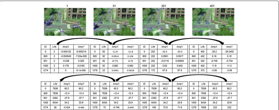
2 - KLT feature tracker: We propose a second strategy that uses the KLT feature tracker [39, 40]. This latter aims to find for each feature point (called also interest point), detected on the video frame(i), a corresponding feature point, detected on the video frame(i+1).
First, we utilize correspondence information between consecutive frames to attribute an identifier for each feature point, detected and tracked on the frame(i), and to save three parameters: Life, AmpX, and AmpY. The three latter respectively describe the number of frames until
Fig. 4Computation of OAS. Example ofaan overlap_score andban accumulation_score
reachingi, the magnitude of the displacement onx, and the magnitude of the displacement ony. In addition, once all the video is processed, we re-propagate, for each point, the values of its parameters from the last frame to the first one. These parameters allow us to classify the feature point as a foreground feature point or a background one. A feature point will be considered a foreground feature point if it has a “Life” parameter in [minlife,maxlife] and “AmpX” or “AmpY” parameters in [minamp,maxamp], whereminlife,maxlife,minamp, andmaxampare given as inputs. Otherwise, it will be a background feature point. Figure 5 illustrates the main idea of this strategy.
Fig. 5KLT feature tracker strategy. Agreen feature pointis detected on both current and previous frames with a very small movement, and ablue pointmoves at least a distance equal to 0.1 between two consecutive frames
negative one if its ROI contains only background feature points or a very limited number of foreground ones.
To use this strategy, we apply Algorithm 3, which takes into account the feature point type in the sample ROI and its predicted label to assign a weight for each sam-ple of subset 2. Table 2 presents the notations utilized in Algorithm 3.
Algorithm 3Observation strategy 2: KLT feature tracker
Input: Subset 2
˘
X(kn+)1
n=1,..,N˘ with associated ROI
posi-tion and size{pi}i=1,..,N˘ into target video-sequence
Target video sequence and associated datasetDt List of parameters:minlife,maxlife,minampand max-amp
List of feature points {FPtsj} relative to each frame j,{FPtsj}j=1..,L
Output: Set{πi}i=1..,N˘ of weights associated to samples
________________________________________
for i=1 toN˘ do πi←0
/* Feature point classification */ FR_FPts←compute_FRPts(pi,{FPtsj}j=1..,L) BK_FPts←compute_BKPts(pi,{FPtsj}j=1..,L) /* Weight assignment */
if((y˘i=pedestrian)&(FR_FPts>BK_FPts))then πi←
FR_FPts FR_FPts+BK_FPts
else if((y˘i = pedestrian)&(FR_FPts < BK_FPts)) then
πi←
BK_FPts FR_FPts+BK_FPts end if
end for
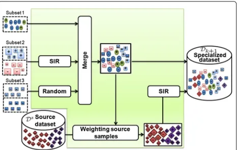
3.2.3 Sampling strategy
This strategy aims to select the samples composing the specialized dataset. Figure 6 depicts the details of its processing. Herein, we present an alternative to previ-ous work, which treated equally the training samples or integrated the sample confidence score in the learning function of the classifier. Our strategy selects the train-ing samples ustrain-ing the SIR algorithm. This latter gives an unweighted set of samples reflecting an input’s weighted set which allows us to consider the associated weights of the training samples without changing the learning function of the classifier.
We approximate, according to (11), the conditional dis-tributionp(X˘k+1|Zk+1)by merging an unweighted target
dataset from subset 2 and a random selection from subset 3. The unweighted target dataset is generated by applying the SIR algorithm on the weighted target dataset provided by the update step.
pX˘k+1|Zk+1
≈X˘∗k(+n1)
n=1,..,N˘k∗+1
∪X˘∗k+(n1)
n=1,..,M˘k∗+1
(11)
Table 2Functions and notations used in Algorithm 3
Notation: definition
-p: It is a spatio-temporal ROI position into the target video
sequence (Dt).
-compute_FRPts(pi,{FPtsj}j=1..,L): It computes the
fore-ground feature points of ROIp.
-compute_BKPts(pi,{FPtsj}j=1..,L): It computes the
Fig. 6Processing details of sampling strategy
whereX˘∗k(+n1)andX˘∗k+(n1)are the selected target samples for the next iteration(k+1)from subsets 2 and 3, respectively. At this level, the posterior distributionp(Xk+1|Z0:k+1)is
approximated according to Eq. 12:
pXk+1|Z0:k+1
≈X∗k(+n1)
n=1,..,N∗
∪X˘∗k(+n1)
n=1,..,N˘k∗+1∪
˘
X∗k+(n1)
n=1,..,M˘k∗+1
(12)
In general, these selected-target samples may contain ones with false labels because they are automati-cally weighted. In addition, they are insufficient to generate an efficient classifier to the target scene. However, the source dataset contains labeled sam-ples that are similar to the target ones and which should be beneficial to the specialization of the classifier.
Thus, we propose to utilize the source distribution to improve the estimation of the target one by select-ing only the source samples that derive from the same target distribution (12). The probability π˘ks(+n1) (weight) that each source sample belongs to the target distribu-tionp(Xk+1|Z0:k+1)is computed using a non-parametric
method based on the KNN algorithm (utilizing the FLANN1library and an L2 distance on features). Based on these probabilities, we apply the SIR algorithm to select the source samples that approximate p(Xk+1|Z0:k+1)
according to Eq. 13:
pXk+1|Z0:k+1
≈Xsk∗+(n1)
n=1,..,N˘ks∗+1 (13)
whereXsk∗+(n1)is the source samplenselected to be in the specialized dataset at the iteration(k+1)andN˘ks∗+1is the
number of the selected source samples. This number is determined using Eq. 14:
˘
Nks∗+1=Ns−N∗+ ˘Nk∗+1+ ˘M∗k+1 (14)
At the end of this step, the new specialized datasetDk+1 is built from both source and target samples (15), and it is used to start the next iteration.
Dk+1=.
X∗k(+n1)
n=1,..,N∗∪
˘
X∗k(+n1)
n=1,..,N˘k∗+1
∪X˘∗k+(n1)
n=1,..,M˘∗k+1∪
Xsk∗+(n1)
n=1,..,N˘s∗ k+1
(15)
The specialization process stops when the ratio between the cardinality of two predicted datasets related to two consecutive iterations exceedsαs(αs= 0.80 fixed
empir-ically in our case). Once the specialization is finished, the obtained classifier can be used for pedestrians’ detection and classification in the target scene based only on their appearance.
4 Experimental results
In this section, we present and discuss the different exper-iments achieved in order to evaluate the performance of our specialization algorithm.
We tested our method on two public traffic videos, the CUHK_Square dataset [16] and the MIT traffic dataset [41], using the same settings as in [15–17, 36]. Also, we have illustrated the results on our Logiroad traffic dataset. Figure 7 shows examples of the three used datasets.
We used the HOG descriptor as a feature vector and we trained the generic and specialized classifiers utilizing the SVMLight2, for both car and pedestrian cases.
4.1 Datasets
- CUHK_Square dataset [16] : It is a video surveillance sequence of 60 min, recording a road traffic scene by a stationary camera. We uniformly extracted (as described in [16]) 452 frames from this video, of which the first 352 frames were used for the specialization and the last 100 frames were utilized for the test. - MIT traffic dataset [41] : A static camera was used to
Fig. 7Three traffic datasets.aCUHK_Square dataset.bMIT traffic dataset.cLogiroad traffic dataset
- Logiroad traffic dataset: It is a record of a traffic scene, which was done by a stationary camera, of almost 20 min. The same reasoning was applied. We uni-formly extracted 700 frames from this video, of which the first 600 frames were used for the specialization and the last 100 frames were utilized for the test.
In our evaluation, we opted for the ground truth pro-vided by Wang and Wang in [15] (noted MIT_P) and by Wang et al. (noted CUHK_P) in [16], to test the detec-tion results of pedestrians on the MIT traffic dataset and on the CUHK_Square dataset, respectively. As there was no available car-annotated database to test the detection results, we proposed annotations relative to cars on both MIT and Logiroad traffic datasets. We note these latter MIT_C and LOG_C, respectively.
We applied the PASCAL rule [42] to compute the true positive rate and the receiver operating charac-teristic (ROC) curve, so as to compare the detectors’ performances. A detection will be accepted if the over-lap area between the detection window and the blob of the ground truth exceeds 0.5 of the union area. A ROC curve presents the pedestrian detection rate for a given false positive rate per image. It is to note that we use the term “specialized classifier” when the con-clusion is true for all classifiers provided by our frame-work independently from the used strategies. Moreover, we apply the specialized classifier based only on object appearance without prior information at the test stage. In addition, the indication of a detection’s rate here-after is always relative to one false positive per image (FPPI = 1).
We collected samples for our source car database from different sets of video sequences3and trained our own car detector. Each sample contained a car in the center. All the samples were normalized into the size of 64×64 pixels and flipped horizontally. The negative samples were cropped randomly from video frames and from the INRIA Person dataset [9] and the INRIA car dataset [43]. We trained and respected the ratio between positive (2100) and negative (12,000) samples, as used in [9] at the initial dataset. Then,
we performed a bootstrap step on the negative images of the INRIA Person dataset. Figure 8a, b illustrates the detections done by our source car detector on the UIUC car dataset [44] and the Caltech cars 2001 (Rear) dataset [45], respectively.
4.2 Convergence evaluation
The comparison of the performances of the specialized classifier at several iterations to that of the generic one demonstrates that our TTL-SMC generates an increase in the detection rate since the first iteration. Figure 9a shows that the specialized classifier performance improves from 26.6 to 60% at the first iteration and from 60% to more than 70% at the fourth iteration on the CUHK_Square dataset. The experiments prove that the performance has improved weakly for the next five iterations. For clarity reasons, we have limited the visualization of the ROC at the tenth iteration.
The Kullback–Leibler divergence (KLD) was another metric evaluation used to measure the convergence of the estimated distribution towards the true target one. We computed the KLD between a set of pedestrians cropped manually from the specialization frames and positive sam-ples of the specialized dataset produced at each iteration.
Fig. 9Evaluation of specialized detector convergence.aDetection performance ROC curves andbKullback–Leibler divergence
The KLD between two sets of realizations was computed as in the work of Boltz et al. [46]. Figure 9b indicates that the KLD decreases until having a minimal variation starting from iteration 4 (corresponding to the stopping iteration) on the CUHK_Square dataset. The same inter-pretation is noticed in the other datasets.
In practice, the convergence of our specialization will be determined when the parameterαs reaches the value
0.8. The parameterαsreflects the ratio between the
num-ber of sample proposals returned at the current iteration and the number of sample proposals in the previous iter-ation. Figure 10 demonstrates that the number of sample proposals stabilizes from iteration 4, which marks the validation of the stopping criterion.
4.3 Effect of sample proposal strategies
To evaluate the effect of sample-proposal strategies, we tested two strategies: one based on three subsets, as described in Section 3.2.1 (noted as SMC_B), and another one, where we were limited to samples of the two first subsets without using background models (noted as SMC_WB). Figure 11 reports the results of our specialization algorithm according to the sample proposal strategies while using the OAS strategy as an observation one. The results of the specialized detector at the first and last iterations are reported.
Although the specialization process converges with the same number of iterations in most of the cases, we notice that the strategy SMC_B needs a little extra time at one iteration on the CUHK_Square dataset and the MIT traf-fic dataset. However, the use of samples extracted from background models leads to an improvement of 6% in the pedestrian detection rate on both datasets. For the case of car detection, we record that both strategies give comparable results on the MIT traffic dataset. Never-theless, the ROC curves of the detection rate on the
Fig. 11Comparison of sample-proposal strategies. Pedestrian detection:aCUHK_Square dataset andbMIT traffic dataset. Car detection:cMIT traffic dataset anddLogiroad traffic dataset
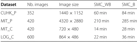
Logiroad traffic dataset show that while the two strategies have the same performance at an FPPI = 1 at the first iteration, the SMC_B strategy improves by 19% in per-formance compared to the SMC_WB at the convergence iteration. Table 3 reports the average time of a specializa-tion’s iteration (sample selection and detector training) on an Intel(R) Core(TM) i7- 3630QM 2.4G CPU machine on each tested dataset with a designed number and size of images.
4.4 Effect of observation strategies
We make a comparison between two observation strate-gies: the OAS and the KLT feature tracker in several cases. This comparison aims to prove the performance of the specialized detector compared to the generic one and to
Table 3Average duration of a specialization’s iteration on several datasets
Dataset Nb. images Image size SMC_WB SMC_B
CUHK_P 352 1440×1152 60 min 84 min
MIT_P 420 4320×2880 210 min 285 min
MIT_C 420 720×480 14 min 28 min
LOG_C 600 864×486 22 min 36 min
show that our proposed specialization is a general frame-work. It can be applied by combining or substituting many algorithms that extract visual context cues from a video recorded by a static camera.
To correctly evaluate the effect of the observation strate-gies, we adopt the SMC_B proposal strategy, which has given the best performance in the tests of Section 4.3 for all the experiments. We note SMC_B_OAS a special-ized detector trained by applying our framework using the SMC_B as a proposal strategy and the OAS as an observation strategy. Also, SMC_B_KLT is noted when the SMC_B and KLT strategies are used.
Fig. 12Comparison of sample-proposal strategies. Pedestrian detection:aCUHK_Square dataset andbMIT traffic dataset. Car detection:cMIT traffic dataset anddLogiroad traffic dataset
detector exceeds that of the generic one by more than 27%. In addition, the curves show that the specialization con-verges after four iterations with a rate of true positives equal to 81%. On the other hand, the SMC_B_KLT detec-tor improves the detection rate by 34%, compared to the generic one.
On the MIT traffic dataset, in the case of pedestrians, our SMC_B_OAS detector ameliorates the detection rate from 10 to 24% at the first iteration and it starts converg-ing from the fourth iteration with 49% of true positive detections. However, the SMC_B_KLT detector converges by a rise of 22% compared to the performance of the generic detector. In the case of cars, we record for both SMC_B_OAS and SMC_B_KLT detectors a raise in the detection rate by 5% at the first iteration, compared to the one of the generic detector. Then, the detection rate of the SMC_B_OAS moves to about 30% at the fourth iter-ation against an increase from 9 to 24% recorded by the SMC_B_KLT detector. We notice that the performance goes up weakly after the fourth iteration corresponding to the stopping iteration in our experiments.
In particular, on the Logiroad traffic dataset, the generic detector presents a detection rate equal to 32%. Nevertheless, our specialized SMC_B_OAS detector gives a detection rate equal to 20% at the first iteration and
then converges with 45% from the fourth iteration. The performance of the SMC_B_KLT detector decreases to 16% at the first iteration and then goes up to 47% at the stopping iteration. We explain the decline at the first iteration by injecting an interest object (failed to be weighted correctly by the spatio-temporal scores because it is temporarily stationary) as a negative sample in the specialized dataset. This means that this sample is detected by the detector but misclassified by the obser-vation strategy, which may disturb the specialization process.
On the other hand, we record a slight fall in most of the final detection rates of the SMC_B_KLT detector, com-pared to those reached by the SMC_B_OAS detector. We can clearly see an improvement generated by our pro-posed specialization framework independently from the strategies used on each step.
Fig. 13Illustration of car detection results. Specialized detector (blue) and generic detector (red). Overlap-accumulation score strategy (2top rows) and KLT feature tracker strategy (2bottom rows). (1 and 3 rows) detections on MIT traffic dataset and (2 and 4 rows) detections on Logiroad traffic dataset
of car detection results to compare the generic and the specialized detectors according to the two observation strategies on both MIT traffic dataset and Logiroad traffic dataset.
4.5 Combination of both observation strategies
In this subsection, we simultaneously apply both observa-tion strategies on the set of proposals returned by the pre-diction step. After that, we combine the weighted datasets as a single one to be an input to the sampling step. Table 4 compares the true detection rates of several specialized detectors with the one given by the generic detector at one false positive per image. It is to note that OAS, KLT, and Fusion refer to the OAS strategy, the KLT feature tracker strategy, and the combination of both strategies, respec-tively. Also, we use it_f and it_c to denote the first iteration and the convergence one.
Table 4 demonstrates again that our framework can be applied utilizing any observation strategy and shows that the combination of the two observation strategies gen-erally improves the classifier performance a bit, but in some cases one strategy gives a better detection rate than Fusion.
4.6 Comparison with state-of-the-art algorithms
In our proposed application, we assume that the target scene is monitored by a static camera. This assumption helps us to extract our visual context cues; however, if other context information is able to be extracted with a mobile camera, our approach may be used.
Considering the fixed assumption, we need annotated video sequences, which are recorded by a stationary
Table 4Detection performance (in percent) of several detectors according to observation strategy used (at FPPI=1)
Specialised detector Generic OAS KLT Fusion
Pedestrian
CUHK it_f 26.6 53.7 46.5 66.5
it_c 81.3 59.6 76.7
MIT it_f 10 24.2 22 26.3
it_c 49 44.1 45.8
Car
MIT it_f 9 15.8 14.7 17.2
it_c 28.7 23.8 31.5
Logiroad it_f 33.5 20.8 16 25.8
camera, in order to compare our proposed approach to the state-of-the-art algorithms. Nevertheless, most of the datasets used specially for car detection or multi-object detection are composed of only still images or video sequences recorded by a moving camera. Hence, we evalu-ate the overall performance of the suggested specialization approach on the CUHK_square and MIT trafic datasets with the following state-of-the-art methods in the case of pedestrian detection.
• Generic [9]: A HOG-SVM detector was built and trained on the INRIA dataset, as proposed in [9] by Dalal and Triggs.
• Manual labeling: A target detector was trained on a set of target labeled samples. This latter was composed by all the pedestrians of the specialization images (pos-itive samples), from which a negative set of samples was extracted randomly taking into account that there was no overlap with pedestrian bounding boxes.
• Nair 2004 [26]: It was a HOG-SVM detector that was created in a similar way to the one suggested in [26], but the HOG descriptor was used as a feature vec-tor and the SVM instead of the Winnow classifier. An automatic adaptation approach picked out the target samples to be added in the initial training dataset using the output of the background subtraction method.
• Wang 2014 [17]: A specific target scene detector was trained on both INRIA samples and samples extracted and labeled automatically from the target scene. The target and the source samples that had a high confi-dence score were selected. The scores were calculated using several contextual cues and the selection was done by a method called “confidence-encoded SVM,” which would favor samples with a high score and would integrate the confidence score in the objective function of the classifier.
• Mao 2015 [19]: A detector was trained on target samples labeled automatically by using tracklets and by information propagation from labeled tracklets to uncertain ones.
Figure 14a shows that the specialized SMC_B_OAS detector significantly exceeds the generic one on the CUHK_Square dataset. The performance soars from 26.6 to 81%. The SMC_B_OAS outperforms the detector trained on target samples, which are labeled manually, by about 31% at an FFPI = 1. However, the target detector with manual labeling slightly exceeds the spe-cialized detector for an FPPI that is less than 0.2. Our SMC_B_OAS CUHK detector also exceeds the three other specialized detectors of Nair (2004), Wang (2014), and Mao (2015) respectively by 45.57, 23.25, and 20%. It is to note that Mao (2015) fairly exceeds our specialized SMC_B_OAS detector for an FFPI less than 0.4.
Fig. 14Overall performance. Comparison of specialized detector with other methods of state-of-art methods:aCUHK_Square dataset andbMIT traffic dataset
On the MIT traffic dataset (Fig. 14b), the detection rate improves from 10 to 47%. The MIT specialized SMC_B_OAS detector exceeds the detector trained on the labeled target samples by about 21%. Compared to Nair 2004’s detector, our specialized SMC_B_OAS detector gives a better detection rate than the one proposed by Nair and Clark for an FPPI less than 1. Otherwise, Nair’s (2004) detector somewhat exceeds our SMC_B_OAS detector. The ROC curves display that our specialized detector gives a comparative detection rate to Wang (2014) detec-tor. It is necessary to mention that shadows, on the MIT video, affect the weighting and the selection of correct positive samples.
Fig. 15Overall performance of same method across datasets
on three methods for a clarity reason. We summarize in Table 5 the pedestrian detection rate of several state-of-the-art detectors related to the CUHK_Square dataset and the MIT traffic dataset for an FPPI = 1. Moreover, we give the gain between our specialized SMC_B_OAS detec-tor and the generic one on the last line. Figure 15 shows that the generic detector has a much better performance on the CUHK_Square dataset than its performance on the MIT traffic dataset and so does our SMC_B_OAS detector. However, Wang (2014) gives practically the same performance on both datasets. This means that the bet-ter generic detector we use in our approach, the betbet-ter specialized detector we get.
It is shown that our SMC specialization process con-verges after only a few iterations on four cases: two for pedestrian detection and two for car detection. In our experiments, we have used different strategies at each step of our filter, which confirms the generalization of our approach.
We notice that the OAS strategy rejects any positive sample having a weight less than the fixed thresholdαp,
Table 5Comparison of detection performance with state-of-the-art detectors at FPPI=1
Detector Dataset
CUHK (%) MIT (%)
Generic [9] 26.60 9.80
Manual labeling 50.36 22.01
Nair 2004 [26] 28.80 42.70
Wang 2014[17] 51.12 49.00
Mao 2015 [19] 61.50
-Our SMC_B_OAS 81.35 48.97
Gain (SMC_B_OAS / generic) 205.82 399.63
which reduces the number of positive samples. Other-wise, a static pedestrian, associated to a negative label, can have a high weight because he/she is detected by the detector at the same location in some frames with a null overlap_score and a high accumulation_score. The KLT feature tracker allows us to select more positive samples but may reduce the negative ones. We note also that the co-execution of both strategies and the combination of outputs (as we did in the test “combination of both strate-gies”) slightly change the performance of the specialized SMC_B_OAS classifier.
Although the proposed observation strategies validate our general framework, the use of other strategies and the combination with other spatio-temporal information can enhance the performance provided by our approach and accelerate the convergence of the specialization process.
5 Conclusions
The suggested TTL-SMC filter automatically specializes a generic detector towards a specific scene. It estimates the unknown target distribution by selecting relevant samples from both source and target datasets. These samples are used to learn a specialized classifier that ameliorates much better the detection rate in the target scene.
Indeed, we have validated the suggested method on sev-eral challenging datasets, applied it on a pedestrian and car detection, and tested it with different strategies. The experiments have demonstrated that the proposed spe-cialization gives a good performance starting from the first iteration. Besides, the results have illustrated that our method gives a comparable performance to Wang’s approach on the MIT traffic dataset and exceeds the state-of-the-art performance on two public datasets.
As a future work, we are going to aggregate our frame-work with fast feature computation techniques to acceler-ate the specialization process, and we are going to extend the proposed approach to a multi-object framework. In addition, we will ameliorate the observation strate-gies with more spatio-temporal information combined together, and we may apply our algorithm to specialize a CNN classifier.
Endnotes
1http://www.cs.ubc.ca/research/flann/
2http://svmlight.joachims.org
3Video sequences provided by Logiroad company
Acknowledgements
Authors’ contributions
HM carried out the studies about transfer learning approaches and theory of the sequential Monte Carlo filter, proposed the general framework and observation strategies, performed the whole experiments, and drafted the manuscript. TC validated the proposed framework in a context of transfer learning approach, supervised and participated in the design of the work, and helped to draft the manuscript. SG participated in the validation of theory and experiments. YG offered the Logiroad videos and helped to formalize the experiments. NEBA supervised the whole work and helped to draft the manuscript. All authors read and approved the final manuscript
Competing interests
The authors declare that they have no competing interests.
Author details
1Institut Pascal, Blaise Pascal University, 24 Avenue des Landais,
Clermont-Ferrand, France.2SAGE ENISo, University of Sousse, BP 264 Sousse
Erriadh, Sousse, Tunisia.3Logiroad, 2 Rue Robert Schuman, Nantes, France.
Received: 9 May 2016 Accepted: 8 November 2016
References
1. S Alvarez, M Sotelo, I Parra, D Llorca, M Gavilán, inProceedings of the World Congress on Engineering and Computer Science (WCECS). Vehicle and pedestrian detection in esafety applications, vol. 2, (2009), pp. 1–6 2. R Danescu, F Oniga, S Nedevschi, Modeling and tracking the driving
environment with a particle-based occupancy grid. ITS.12(4), 1331–1342 (2011)
3. F Han, Y Shan, R Cekander, HS Sawhney, R Kumar, inPerformance Metrics for Intelligent Systems (PMIS) 2006 Workshop. A two-stage approach to people and vehicle detection with hog-based SVM (Citeseer, 2006), pp. 133–140
4. B-F Lin, Y-M Chan, L-C Fu, P-Y Hsiao, L-A Chuang, S-S Huang, M-F Lo, Integrating appearance and edge features for sedan vehicle detection in the blind-spot area. ITS.13(2), 737–747 (2012)
5. S Sivaraman, MM Trivedi, Vehicle detection by independent parts for urban driver assistance. ITS.14(4), 1597–1608 (2013)
6. D Sun, J Watada, inIntelligent Signal Processing (WISP), 9th International Symposium on. Detecting pedestrians and vehicles in traffic scene based on boosted HOG features and SVM (IEEE, 2015), pp. 1–4
7. Q Yuan, A Thangali, V Ablavsky, S Sclaroff, Learning a family of detectors via multiplicative kernels. PAMI.33(3), 514–530 (2011)
8. X Zhang, N Zheng, inIntelligent Transportation Systems (ITSC), 13th International IEEE Conference on. Vehicle detection under varying poses using conditional random fields (IEEE, 2010), pp. 875–880
9. N Dalal, B Triggs, in2005 IEEE Computer Society Conference on Computer Vision and Pattern Recognition (CVPR). Histograms of oriented gradients for human detection, vol. 1 (IEEE, 2005), pp. 886–893
10. P Dollár, Z Tu, P Perona, S Belongie, inBritish Machine Vision Conference, BMVC 2009, Proceedings. Integral channel features (British Machine Vision Association, 2009), pp. 1–11
11. P Dollár, S Belongie, P Perona, inBritish Machine Vision Conference, BMVC 2010, Proceedings, vol. 2, issue 3. The fastest pedestrian detector in the west (British Machine Vision Association, 2010), pp. 1–11
12. P Dollár, R Appel, S Belongie, P Perona, Fast feature pyramids for object detection. PAMI.36(8), 1532–1545 (2014)
13. PF Felzenszwalb, RB Girshick, D McAllester, inThe Twenty-Third IEEE Conference on Computer Vision and Pattern Recognition, CVPR 2010. Cascade object detection with deformable part models (IEEE, 2010), pp. 2241–2248 14. P Felzenszwalb, D McAllester, D Ramanan, inComputer Vision and Pattern
Recognition, CVPR 2008, IEEE Conference on. A discriminatively trained, multiscale, deformable part model (IEEE, 2008), pp. 1–8
15. M Wang, X Wang, inComputer Vision and Pattern Recognition (CVPR), 2011 IEEE Conference on. Automatic adaptation of a generic pedestrian detector to a specific traffic scene (IEEE, 2011), pp. 3401–3408
16. M Wang, W Li, X Wang, inComputer Vision and Pattern Recognition (CVPR), 2012 IEEE Conference on. Transferring a generic pedestrian detector towards specific scenes (IEEE, 2012), pp. 3274–3281
17. X Wang, M Wang, W Li, Scene-specific pedestrian detection for static video surveillance. PAMI.36(2), 361–374 (2014)
18. X Li, M Ye, M Fu, P Xu, T Li, Domain adaption of vehicle detector based on convolutional neural networks. IJCAS.13(4), 1020–1031 (2015) 19. Y Mao, Z Yin, in2015 IEEE Winter Conference on Applications of Computer
Vision (WCACV). Training a scene-specific pedestrian detector using tracklets (IEEE, 2015), pp. 170–176
20. H Maâmatou, T Chateau, S Gazzah, Y Goyat, N Essoukri Ben Amara, in Proceedings of the 11th Joint Conference on Computer Vision, Imaging and Computer Graphics Theory and Applications (VISIGRAPP 2016) - Volume 4: VISAPP. Transductive transfer learning to specialize a generic classifier towards a specific scene (SciTePress, 2016), pp. 411–422
21. A Doucet, N De Freitas, N Gordon,Sequential Monte Carlo methods in practice. (Springer Science + Business Media, New York, 2001) 22. M Isard, A Blake, Condensation—conditional density propagation for
visual tracking. IJCV.29(1), 5–28 (1998)
23. I Smal, W Niessen, E Meijering, in4th IEEE International Symposium on Biomedical Imaging: From Nano to Macro. Advanced particle filtering for multiple object tracking in dynamic fluorescence microscopy images (IEEE, 2007), pp. 1048–1051
24. X Mei, H Ling, Robust visual tracking and vehicle classification via sparse representation. PAMI.33(11), 2259–2272 (2011)
25. C Rosenberg, M Hebert, H Schneiderman, inApplication of Computer Vision, 2005. WACV/MOTIONS ’05 Volume 1. Seventh IEEE Workshops on. Semi-supervised self-training of object detection models (IEEE Press, 2005), pp. 29–36
26. V Nair, JJ Clark, inComputer Vision and Pattern Recognition (CVPR), Proceedings of the 2004 IEEE Conference on. An unsupervised, online learning framework for moving object detection, vol. 2 (IEEE, 2004), pp. II–317
27. A Levin, P Viola, Y Freund, inComputer Vision, 2003. Proceedings. Ninth IEEE International Conference on (ICCV). Unsupervised improvement of visual detectors using cotraining (IEEE, 2003), pp. 626–633
28. T Chesnais, N Allezard, Y Dhome, T Chateau, inVISAPP 2012 - Proceedings of the International Conference on Computer Vision Theory and Applications, Volume 1. Automatic process to build a contextualized detector (SciTePress, 2012), pp. 513–520
29. SJ Pan, Q Yang, A survey on transfer learning. KDE.22(10), 1345–1359 (2010)
30. T Tommasi, F Orabona, B Caputo, inComputer Vision and Pattern Recognition (CVPR), 2010 IEEE Conference on. Safety in numbers: learning categories from few examples with multi model knowledge transfer (IEEE, 2010), pp. 3081–3088
31. Y Aytar, A Zisserman, in2011 International Conference on Computer Vision (ICCV). Tabula rasa: model transfer for object category detection (IEEE, 2011), pp. 2252–2259
32. SJ Pan, IW Tsang, JT Kwok, Q Yang, Domain adaptation via transfer component analysis. NN.22(2), 199–210 (2011)
33. B Quanz, J Huan, M Mishra, Knowledge transfer with low-quality data: a feature extraction issue. KDE.24(10), 1789–1802 (2012)
34. JJ Lim, R Salakhutdinov, A Torralba, inAdvances in Neural Information Processing Systems (NIPS). Transfer learning by borrowing examples for multiclass object detection, (2011), pp. 118–126
35. K Tang, V Ramanathan, L Fei-Fei, D Koller, inAdvances in Neural Information Processing Systems (NIPS). Shifting weights: adapting object detectors from image to video, (2012), pp. 638–646
36. X Zeng, W Ouyang, M Wang, X Wang, inEuropean Conference on Computer Vision (ECCV). Deep learning of scene-specific classifier for pedestrian detection (Springer, 2014), pp. 472–487
37. K Ali, D Hasler, F Fleuret, inComputer Vision and Pattern Recognition (CVPR), 2011 IEEE Conference on. Flowboost–appearance learning from sparsely annotated video (IEEE, 2011), pp. 1433–1440
38. M Oquab, L Bottou, I Laptev, J Sivic, inProceedings of the IEEE conference on Computer Vision and Pattern Recognition (CVPR). Learning and transferring mid-level image representations using convolutional neural networks (IEEE, 2014), pp. 1717–1724
39. C Tomasi, T Kanade,Detection and tracking of point features. (School of Computer Science, Carnegie Mellon Univ. Pittsburgh, Pittsburgh, 1991) 40. J Shi, C Tomasi, inComputer Vision and Pattern Recognition (CVPR), 1994
IEEE Conference on. Good features to track (IEEE, 1994), pp. 593–600 41. X Wang, X Ma, WEL Grimson, Unsupervised activity perception in
42. M Everingham, L Van Gool, CK Williams, J Winn, A Zisserman, The pascal visual object classes (VOC) challenge. IJCV.88(2), 303–338 (2010) 43. P Carbonetto, Dorkó, C Schmid, H Kück, N De Freitas, Learning to
recognize objects with little supervision. IJCV.77(1-3), 219–237 (2008) 44. S Agarwal, A Awan, D Roth, Learning to detect objects in images via a
sparse, part-based representation. PAMI.26(11), 1475–1490 (2004) 45. B Philip, P Updike, Caltech Computational Vision Caltech Cars 2001 (Rear).
http://www.vision.caltech.edu/archive.html
46. S Boltz, E Debreuve, M Barlaud, High-dimensional statistical measure for region-of-interest tracking. IP.18(6), 1266–1283 (2009)
Submit your manuscript to a
journal and benefi t from:
7Convenient online submission
7Rigorous peer review
7Immediate publication on acceptance
7Open access: articles freely available online
7High visibility within the fi eld
7Retaining the copyright to your article