Interest rate dynamics and monetary policy implementation in Switzerland

© Swiss Society of Economics and Statistics 2010, Vol. 146 (1) 313–340 a We would like to thank Katrin Assenmacher-Wesche, Sebastien Kraenzlin, Antoine Martin,

Dewet Moser, Angelo Ranaldo, participants of an internal SNB seminar and in particu-lar Martin Schlegel for support and helpful comments. This research was supported by the Deutsche Forschungsgemeinschaft through the CRC 649 “Economic Risk”. Contact: puriya. abbassi@uni-mainz.de, dieter.nautz@fu-berlin.de, christian.offermanns@fu-berlin.de. 1 The London Interbank Offered Rate (Libor) is an indicative interest rate at which an individual

contributor panel bank could borrow funds, were it to do so by asking for and then accepting interbank offers in reasonable market size, just prior to 12 a. m. CET. It serves as the main instrument for benchmarking short-term rates and is used as the basis for settlement of inter-est rate contracts on many of the world’s major futures and options exchanges. For further details see www.bbalibor.com.

Implementation in Switzerland

Puriya Abbassi, Dieter Nautz and Christian J. Offermanns

JEL-Classification: E52, E58

Keywords: Implementation of Monetary Policy, Operational Targets of Monetary Policy, Three-Month Rate Targeting, Financial Crisis

1. Introduction

The way monetary policy is implemented by the Swiss National Bank (SNB) dif-fers from the procedures of most other central banks. Since the introduction of the SNB’s new monetary policy framework in 1999, the maturity of the opera-tional target of monetary policy has been a distinguishing feature of the SNB’s operational framework. While other central banks use more or less explicit tar-gets for the overnight rate to signal the policy-intended interest rate level, the SNB announces a target range for the three-month (3M) Libor.1 This paper investigates the working and the consequences of the SNB’s unique operational framework for the behavior of Swiss money market rates before and during the financial crisis.

three-month rate targeting might lead to similar outcomes in normal times, when large shocks are absent and spreads between interbank money market rates are low and stable. During the financial crisis, however, the behavior of Swiss interest rates suggests that the SNB’s three-month rate targeting might have some additional features that could make it even interesting for other central banks.

The SNB manages the 3M Libor through both, words and deeds. First of all, the announced target rate itself should have an influence on the Libor. Moreo-ver, since the current Libor will also depend on the expected path of the target range, the management of market expectations via e.g. interviews and speeches is of particular importance for the SNB, see e.g. Schlegel (2009). The SNB’s communication of current and future target rates is substantiated by a very active liquidity management. The most important policy instrument are daily repo auctions with one-week maturity. The repo volume allotted in these auc-tions determines the level of reserves and, in addition, the pre-announced repo rate governs the one-week repo rate in the interbank money market. As a result, the repo rate can be seen as the SNB’s intermediate policy rate to manage the 3M Libor.

In accordance with the central role of the 1W repo rate and the 3M Libor in the SNB’s operational framework, our empirical analysis focuses on how these inter-est rates respond to various policy-relevant factors including e.g. deviations of the Libor from the target, changes in risk premia, market expectations, and the SNB’s supply of reserves. In order to capture a possible change in interest rate dynamics and the SNB’s monetary policy, both interest rate equations are estimated for the period before and after the outbreak of the financial crisis separately.

Our paper builds on earlier empirical contributions on the implementation of Swiss monetary policy. The closest reference to our work is Jordan and Kugler (2004), who also employ error-correction-type equations to explore the adjust-ment of Libor rates to deviations from the target. Jordan, Ranaldo, and Söder-lind (2009) propose a regime-dependent model to allow for a different response of the Libor before and during the financial crisis. Their findings confirm that repo operations and changes in the target rate are instrumental for the imple-mentation of the SNB’s monetary policy.

2 Exceptionally, the SNB deviated from this rule due to technical reasons. In 6 March, 2003, for instance, the SNB temporary narrowed down the target range from 100 to 75 basis points and intended to keep the 3M Libor rate at around 0.25%, i.e. at the lower end of the new target range.

3 Starting in 8 October 2008, the 3M Libor topped its upper bound for a period of roughly 10 days. With the unexpected 50 basis point change on 6 November 2008, and the 100 basis point change on 20 November 2008, the 3M Libor again exceeded the ceiling of its corridor each for a single day. This is (at least for the two latter cases) due to the timing of the Libor fixing which has been prior to the decision announcements.

2. Three-Month Rate Targeting

In this section, we will have a first look at the implementation of the SNB’s three-month rate targeting. Section 2.1 describes how targets for the three-three-month rate are set and provides a preliminary assessment of their empirical performance. In Section 2.2 we discuss the specific role of interest rate expectations and the SNB’s target corridor. Section 2.3 describes how the SNB uses regular open market operations to steer the three-month rate within the corridor. Section 2.4 compares the interest rate management of the SNB and the ECB during the financial crisis.

2.1 A First Look at the Data

At each Thursday in the third week of March, June, September and December the SNB provides an assessment and addresses its decisions, concerns, views and outlook about monetary and economic developments. In particular, a target cor-ridor of about 100 basis points is announced for the 3M Libor where the aimed level is typically determined by the middle of the corridor.2 Target changes have always been communicated with an immediate effect.

Although both mean and standard deviation of the spread have increased, pre-liminary data analysis already indicates that the SNB’s three-month rate target-ing even worked durtarget-ing the financial crisis.

2.2 Rate Expectations and the Target Corridor

If policy is implemented via a target for a particular interest rate, large and persist-ent deviations of that rate from its target must be avoided since those lead either to wrong signals about the intended rate or question the ability of the central

Figure 1: The Target Range of the SNB

0 1 2 3 4 5

2000 01 02 03 04 05 06 07 08 09

3M Libor (r) target rate (r*) target range

Notes: The shaded area refers to the crisis period as of 9 August, 2007.

Table 1: Libor Spread: Descriptive Statistics

r − r*

sample mean median SD obs. # out

3 Jan 2000–8 Aug 2007 0.02 0.01 0.10 1982 0

9 Aug 2007–30 Jun 2009 0.10 0.06 0.14 495 12

bank to keep interest rates on track, see e.g. Hassler and Nautz (2008). Typi-cally, central banks augment point targets for interest rates by a target corridor in order to deemphasize small and irrelevant deviations from the target. In case of overnight rate targeting, the corridor is often defined by the rates of standing facilities which bound the volatility of the overnight rate in a very simple and effi-cient way. In particular, with standing facilities the overnight rate will not leave its corridor simply due to arbitrage reasons. At first glance, the implementation of monetary policy via overnight rate and three-month rate targeting seem to be very similar since both approaches involve interest rate targets and corridors. However, if the emphasis of monetary policy is shifted from the overnight rate to a longer-term interest rate, this is not the whole story. For the SNB’s opera-tional framework, the role of rate expectations and the raopera-tionale of an interest rate corridor are different.

Consider, for example, the deviations of the 3M Libor from the target in 2006 displayed in Figure 2. Obviously, these marked and persistent target deviations do not indicate bad communication or a failure of interest rate control. In con-trast, it is a direct consequence of the expectations hypothesis of the term struc-ture that an anticipated and well-communicated change of the three-month rate target must lead to expectations-driven target deviations. In contrast to overnight rates, the three-month rate cannot simply stay on the old target level until the day of the rate change.4

This distinguishing feature of three-month rate targeting has two important implications. First, it provides a further rationale for the announcement and the width of a target corridor. Provided that target rate changes do not exceed 50 basis points, a corridor of 100 basis points guarantees that the three-month rate will be on target even immediately before an anticipated rate change. Second, in case of overnight rates, expected changes of the target rate can only be important several days before the implementation of the interest rate change. In contrast, as long as regular central bank meetings are scheduled at least every three months, rate expectations influence Swiss’ three-month rates permanently, at each day between two meetings. Therefore, deviations of the three-month rate from the current target are not a feasible measure to evaluate the current interest rate level and the success of the targeting efforts by the central bank.

5 See appendix for the complete picture of the expectations-adjusted three-month rate target.

A more appropriate measure for the policy intended three-month rate, rt ,

∗

is a convex combination of the current and the expected future target rate:

= ( ),

t t t t t

r∗ r∗+w f −r∗

(1)

where f_t denotes the expected future target rate, and w_t represents a weighting factor. This weight increases (linearly) from zero to one as the expected sub-sequent target rate becomes more relevant over time. In the following, we use the interest rate on the (three-month) next future to proxy the expected future target rate. Using the future rate to calculate the implicit policy intended level of the three-month rate assumes that market expectations are generally in line with the plans of the SNB. Figure 2 shows the expectations-adjusted three-month rate target and the actual three-three-month rate for the time period from 2006 until the beginning of the financial crisis.5 _{The small deviations between}

Figure 2: Target Deviations in Times of Rate Change Expectations

0.4 0.8 1.2 1.6 2.0 2.4 2.8

2006Q2 2006Q3 2006Q4

3M Libor (r) target range target rate (r*)

expectation adjusted target

6 See Kraenzlin and Schlegel (2009) for a comprehensive survey of the SNB’s operational framework and an empirical analysis of banks’ bidding behavior in repo auctions.

7 From 2001 to 2003 one-week repo auctions were used in 27% of the auctions, the SNB has used this maturity in approximately 90% of the cases ever since 2004, see Schlegel (2009).

both interest rates reveal that three-month rate targeting worked particulary well in this period.

Shifting the focus of monetary policy from overnight rates to longer-term rates increases the role of rate expectations and, thus, the importance of the central bank’s expectations management. The SNB governs market expecta-tions on upcoming target changes in several ways, including speeches and inter-views, see e.g. Schlegel (2009). Yet, the assumption of perfect anticipation of interest rate changes might be too strong. Following Jordan, Ranaldo, and Söderlind (2009), we therefore include a measure of interest surprises into our empirical analysis. According to Hamilton (2009), daily three-month future rates capture daily changes in markets expectations of central banks near-term policy rate. Therefore, our surprise variable, surpr, is defined as the change in the three-month future on the day of SNB’s regular monetary policy assessment meetings and zero otherwise.

2.3 The Repo Auctions of the SNB and the Repo Rate

In addition to the management of interest rate expectations, repo auctions are the SNB’s main instrument to steer the 3M Libor.6 _{The results and refinancing} con-ditions in these auctions determine the liquidity situation and, thus, the interest rates in the interbank money market. Probably reflecting both, the SNB’s greater flexibility in the short-term money market (compare Baltensperger, Hilde-brand, and Jordan, 2007) and the more ambitious operational target, the SNB is rather active in the money market. In the last years repo transactions with vari-ous maturities have been conducted on a daily basis. The most prevalent auction format are fixed rate tenders with a maturity of one week.7

8 For instance, in the period after 6 October 2008, the widened spread between the 1W repo rate and the SNB’s repo rate as depicted in Figure 3 reflects the impact of such additional measures.

monetary transmission process. In the following empirical analysis of Swiss inter-est rate dynamics, we will use the repo rate rather than the auction rate as the SNB’s policy rate because the secondary market rate repo also reflects the impact of other monetary policy actions including the volume of allotted reserves or additional fine-tuning operations.8

The SNB’s Supply of Reserves

If banks’ total bids exceed the SNB’s intended supply of reserves, the SNB rations all bids above a minimum amount proportionally. Following Jordan and Kugler (2004), our empirical analysis of the SNB’s interest rate management considers the possible impact of the SNB’s allotment decisions.

Data on the SNB refinancing auctions is available from 8 January 2001 onwards. The upper part of Figure 4 depicts the aggregate allotment volume

Figure 3: The SNB’s Policy Instrument

–.4 –.2 .0 .2 .4

0 1 2 3 4

2001 02 03 04 05 06 07 08 09

1W repo rate SNB repo rate

1W repo rate - SNB repo rate

9 On some few occasions, the SNB did not perform a one-week repo auction. In all these cases, we filled the data with the repo rate of the prevailing maturity. Following Jordan and Kugler (2004), there is no difference in the impact of repo auctions with different maturities.

and the total bid amount of all repo operations with one week maturity.9 _Since 2004, the bid volumes have become larger because of the increased importance of one-week repo auctions in the set of the SNB’s policy instruments. During the financial crisis, bids decreased because banks anticipated the full allotment policy of the SNB. In the lower part of the Figure, we displayed the resulting cover to bid ratio, cbr, defined as the ratio between total allotment and total bids. Note that this ratio is far from constant and, typically, not easy to predict from the perspective of a single bank. In particular, there is no obvious upward trend in the cover-to-bid ratio. In contrast to the ECB, the SNB did not experience that

Figure 4: Bids and Allotments in Repo Auctions

0.0 0.2 0.4 0.6 0.8

1.0 0

50,000 100,000 150,000 200,000

01 02 03 04 05 06 07 08 09

cover to bid ratio total allotment total amount of bids

10 Before the crisis, even target deviations of only a few basis points lead to discussions about the ECB’s monetary setup, see e.g. Linzert and Schmidt (2008).

banks started to increasingly exaggerate their bids in order to circumvent the rationing, see Nautz and Oechssler (2006). One explanation for the working of the SNB’s fixed rate tender format is suggested by the time series of the spread between the fixed rate and the related market rate (repo), see Schlegel (2009). Figure 3 shows that the spread between both interest rates has been small but rather volatile and with changing sign. Therefore, overbidding in SNB’s repo auc-tions might have been avoided because banks could not be sure to make profits by reselling excess reserves on the secondary market.

2.4 Interest Rate Targeting in the Financial Crisis: SNB and ECB

Since August 2007, the environment of an extreme nervousness among money market players started to have a great impact on global money markets. As a result, the concerns about liquidity, market and credit risk exposure – as reflected by the spread between the 3M Libor and the overnight index swap (OIS) rate – skyrocketed for major currencies, see Figure 5.

During the financial crisis many central banks experienced unusual difficulties in implementing the policy-intended levels of short-term interest rates. For example, before the crisis the spread between the ECB’s operational target, i.e. the overnight rate Eonia, and the policy rate, i.e. the minimum bid rate of the main refinancing operation, has been very small and to a large extent under the ECB’s control.10 _In this calm period, risk premia were small and future short-term rates rather easy to predict. The spread between the 3M Euribor and the Eonia was under control and in line with policy intentions. This picture changed dramatically in the course of the financial crisis, see Figure 6. The massive liquidity injections of the ECB cer-tainly helped to stabilize the banking sector but decoupled the Eonia from the min-imum bid rate. Since the Lehman breakdown, banks have used the ECB’s deposit facility on a large scale to deposit excess reserves. As a result, the deposit rate has become the new reference rate for the Eonia. Although the ECB did not officially announce a new interest rate targeting regime, there is certainly an increased con-cern about the level of longer-term money market rates. The observed change in the ECB’s interest rate management might have led to some confusion of market participants about the policy intended interest rate level.

abandon its operational target. Mean and volatility of the spread between the 3M Libor and its target have only slightly increased during the financial crisis, see Section 2.1. Figure 6 shows that the SNB decreased its repo rate dramatically in order to keep the 3M Libor close to its target. The transparency of the SNB’s interest rate policy might have contributed to keep the risk premia revealed by the Libor-OIS spreads relatively low, see Figure 5.

3. Monetary Policy Implementation and Interest Rate Dynamics:

Empirical Results

In accordance with the SNB’s operational framework of monetary policy, the following empirical analysis focusses on the dynamics and adjustment processes of the 1W repo rate and the 3M Libor. For both interest rates, error-correction type equations are employed to estimate how the interest rates respond to various policy-relevant factors, see Jordan and Kugler (2004). Due to data availability,

Figure 5: Risk Premia in the Financial Crisis

0.0 0.5 1.0 1.5 2.0 2.5 3.0 3.5 4.0

1/2007 7/07 1/08 7/08 1/09

CHF EUR USD

Figure 6: Swiss and Euro Area Interest Rates in the Crisis

0 1 2 3 4 5 6

Eonia deposit facility marginal lending facility

MRO’s minimum bid rate/fixed rate 3M Euribor

0.0 0.5 1.0 1.5 2.0 2.5 3.0 3.5

7/2007 1/08 7/08 1/09

7/2007 1/08 7/08 1/09

1W repo rate target range target rate 3M Libor

11 In fact, while unit root tests indicate that both interest rates are integrated of order one, the term spread can be assumed to be stationary. For similar results for euro area and U.S. inter-est rates, see e.g. Nautz and Offermanns (2007) and Sarno and Thornton (2003).

we use daily data ranging from 8 January 2001 until 30 June 2009. To control for the effects of the financial crisis on interest rate dynamics, both interest rate equa-tions are estimated for the period before and after 9 August, 2007 separately.

3.1 The Dynamics of the Policy Instrument

We begin with the estimation of the adjustment equation of the SNB’s policy rate, i.e. the 1W repo rate (of the secondary money market), which is specified as follows:

5

1 1

=1

5 5

=0 =1

= ( ) ( )

ln .

t t t j t j

j

j t j j t j t t t

j j

repo r r r repo risk

r repo cbr surpr u

α β γ

δ ϕ θ φ μ

∗

− − −

∗

− −

Δ − + − + Δ

+ Δ + Δ + + + +

∑

∑

∑

(2)

12 A complete presentation of the estimation results is shown in the Appendix.

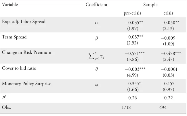
Table 2: The Adjustment Equation of the SNB’s Policy Instrument

Variable Coefficient Sample

pre-crisis crisis

Exp.-adj. Libor Spread _{α −0.035**}

(1.97)

−0.050** (2.13)

Term Spread _β 0.037**

(2.52) −0.009_(1.09)

Change in Risk Premium 5

1 j

j=γ

∑

Cover to bid ratio _{θ −0.003***}

(4.59)

−0.0001 (0.03)

Monetary Policy Surprise _φ 0.355*

(1.66)

0.157 (0.97)

R2

0.26 0.22

Obs. 1718 494

Notes: The table refers to Equation (2):

5

1 1

=1

= ( *) ( ) ln .

t t t j t j t t t

j

repo αr r − βr repo − γ risk− θ cbr φsurpr u

Δ − + − +

∑

Notes: ***,**,* indicate significance at the 1%, 5%, 10% level. Absolute t-statistics in parentheses are computed according to Newey and West (1987). The pre-crisis sample runs from 3 January 2000 to 8 August 2007, the crisis sample ends in 30 June 2009. The full set of estimation results for this equation can be found in Table 5 in the appendix.

By contrast, the adjustment coefficient of the term spread (β) clearly differs before and during the financial crisis. Before the crisis, the estimated response of the repo rate to the term spread is in line with the predictions of the expecta-tions theory of the term structure. During the crisis, however, the estimate of _βˆ is not significant and even implausibly signed. In the financial crisis, increases in the 3M Libor were certainly not due to expected future increases of the 1W repo rate but resulted from increases in risk premia. Therefore, the breakdown of the standard expectations-based equilibrium relation between the 1W repo rate and the 3M Libor reflects the SNB’s active interest rate management via the 1W repo rate.

In both periods there is a significant reaction of the repo rate to changes in the risk premium. Interestingly, the long-run effect of changes in risk on the repo rate, 5

=1 ,

j γj

∑ is largely unaffected by the crisis. In both periods, increases in the risk premium were followed by a decreasing repo rate. Given the structural stabil-ity of the SNB’s response to changes in risk, the large and persistent risk premia during the crisis explain a major part of the behavior of repo rates.

As expected, large cover-to-bid ratios indicate a generous liquidity supply and lead to decreasing repo rates in the pre-crisis sample. In the crisis, this plausible effect disappears because cover-to-bid ratios were typically one as a result of the full allotment policy of the SNB. Finally, we find no significant impact of the surprise variable on the repo rate. This can be partly explained by the maturity mismatch between the one week rate and the surprise measure which recurs to the three-month next future. However, it also shows that the one week rate car-ries only little information about the monetary policy stance, and thus, is little affected by the SNB’s longer-term assessments.

3.2 The Dynamics of the Operational Target

Let us now turn to the empirical analysis of the 3M Libor dynamics. Similar to Jordan and Kugler (2004) and the adjustment equation employed for the repo rate, the analysis of the 3M Libor dynamics is based on an error-correction-type adjustment equation:

1 1 1 1

5 5 5

=0 =1 =1

= ( ) ( )

.

t t t t t

j t j j t j j t j t t

j j j

r r r r repo

r repo r surpr v

α β

δ ϕ ψ φ μ

∗

− − − −

∗

− − −

Δ − + −

+

∑

∑

∑

The response of r_t to the error-correction terms reflects the two channels, words and deeds, of the SNB’s interest rate management. First, a successful expectations management of the SNB should imply that the 3M Libor adjusts significantly to the expectation-adjusted target rate rt .

∗

Second, if the SNB can actually influ-ence the 3M Libor via the repo rate, there should be a significant response of the 3M Libor to the repo rate via the term spread, (r − repo).

The SNB announces the conditions of the repo auction at 9 a. m. CET on each operation day and invites banks to submit their bids. The auction is closed at 9.10 a. m. CET and individual results are being announced at (roughly) 9.20 a. m. CET including both the total bid and total allotment. The Libor fixing occurs at 12 a. m. CET.

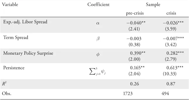
Table 3: The Adjustment Equation for the 3M Libor

Variable Coefficient Sample

pre-crisis crisis

Exp.-adj. Libor Spread _{α −0.040**}

(2.41)

−0.026*** (3.59)

Term Spread _{β −0.003}

(0.38)

−0.007*** (3.42)

Monetary Policy Surprise _φ 0.390**

(2.00)

0.282*** (2.79)

Persistence 5

1 j

j=ψ

∑

0.613*** (10.33)

R2

0.26 0.87

Obs. 1723 494

Notes: The table refers to Equation (3):

5

1 1

=1

= ( *) ( ) .

t t t j t j t t

j

r αr r ₋ βr repo ₋ ψ r₋ φsurpr v

Δ − + − +

∑

The full set of estimation results for this equation can be found in Table 6 in the Appendix. Note that the R2

in the crisis period is inflated by dummy variables capturing two outliers in November and December 2008. For further notes, see Table 2.

rate clearly indicates the existence of the “words channel” of monetary policy implementation. Remarkably, the size of the coefficient is almost the same in both periods. The channel of steering the three-month rate by signals about the current and future level of the target rate seems to be unaffected by the financial crisis. Focusing on the dynamics of the adjustment equation for the 3M Libor, the half-life period of a shock to the expectations-adjusted target rate r∗ is about 19 days before and 23 days during the crisis.

The adjustment coefficient β of the 3M Libor to the term spread is significantly negative in the crisis period and insignificant before. This suggests that the role of the 1W repo rate and, thus, of the “deeds channel’’ of monetary policy implemen-tation has increased in the crisis period. Note that the significant adjustment of the 3M Libor to the repo rate cannot be explained by simple expectations effects. In fact, a typical finding of the empirical literature on interest rate dynamics is that longer-term interest rates are weakly exogenous and do not adjust to interest rates with shorter maturities, see e.g. Sarno and Thornton (2003), and Has-sler and Wolters (2001).

Our empirical results suggest that the working of the SNB’s interest rate man-agement in the financial crisis can be illustrated as follows. Suppose that an increase in the risk premium (Δrisk > 0) had caused an unwished increase in the 3M Libor above its expectations-adjusted target, i.e. r− >r∗ 0. According to Table 2, the SNB responds to the equilibrium deviation with a decrease in the 1W repo rate which in turn will increase the term spread r − repo. Finally, Table 3 shows how the increased term spread helps to bring the 3M Libor back to target.

Two further results shown in Table 3 are worth noting. First, there has been a significant increase in the persistence of the 3M Libor during the crisis. Second, while the surprise variable played no role for the dynamics of the repo rate, our estimates show that monetary policy surprises have a significant impact on the three-month rate. This confirms the different functions of the two interest rates: it is the three-month rate through which the SNB’s monetary policy stance is transmitted, and not the one week rate.

3.3 The Interest Rate Management of the ECB

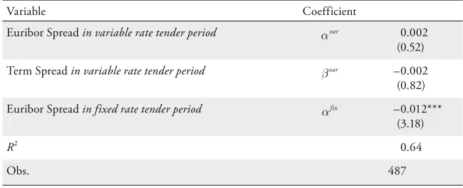
investigate to what extent the ECB’s monetary policy implementation has become equivalent to the three-month rate targeting approach of the SNB.

Since the beginning of the financial crisis in August 2007, the interest rate management of the ECB can be divided into two regimes. In the first year of the crisis, until the Lehman breakdown in September 2008, the ECB still tried to keep the Eonia close to its key policy rate, i.e. the minimum bid rate of its main refinancing operation (MRO). However, the ECB also began to be explic-itly concerned about stabilizing longer-term money market rates. To that aim, the ECB increased drastically the volume and frequency of its longer-term refi-nancing operations (LTROs). While the share of LTROs in total refirefi-nancing was 33% in the first half of 2007, it rose to more than 60% in the beginning of 2008, see European Central Bank (2009, p. 79). All these LTROs had been conducted as variable rate tenders. In contrast to MROs, however, the LTROs were performed without a minimum bid rate. Therefore, the ECB sent no signal about the intended longer-term repo rate and thus, its impact on Euribor rates has been limited.

Banks became more and more reluctant to lend to each other and the distri-bution of liquidity was severely impaired. Even solvent banks were observed to experience problems with refinancing through the interbank money market. As a result, banks increased their recourse to the ECB’s refinancing operations and the average MRO interest rate jumped to more than 70 basis points above the minimum bid rate. Moreover, Libor-OIS spreads revealed that particularly the 3M Euribor was inflated by a huge risk premium. In view of these extreme dis-turbances, the ECB partly abandoned the overnight rate Eonia as its operational target (see Section 2.4) and adjusted its operational framework in several ways, see European Central Bank (2009). In particular, the ECB switched from the variable rate to the fixed rate tender format with full allotment in all refinancing operations. Moreover, the repo rate set by the ECB was the same for all maturi-ties. Therefore, from 15 October 2008 onwards, by announcing a fixed rate for liquidity provision in the three-month horizon, the ECB basically published a target for the 3M Euribor.

terms show that the ECB’s impact on the 3M Euribor has been only weak in the variable rate tender regime. By contrast, the adjustment coefficient of the fixed rate regime is highly significant and plausibly signed. In contrast to the SNB, the ECB not only sends signals about the policy intended level of the 3M Euribor. Rather, using fixed rate tenders with full allotment, the ECB directly intervenes in the three-month money market segment. Apparently, the introduction of fixed rate tenders together with the commitment of full allotment at the target rate sig-nificantly improved the ECB’s control over longer-term money market rates.

4. Concluding Remarks

Over the last 10 years, a distinguishing feature of the SNB’s monetary policy framework has been the announcement of a target corridor for the 3M Libor. This paper investigated the empirical relevance of this target for the interest rate dynamics of the 3M Libor and 1W repo rate, i.e. the SNB’s main policy rate. Our empirical results show that the SNB controls the 3M Libor through

Table 4: The Adjustment of the 3M Euribor in the Crisis

Variable Coefficient Euribor Spread in variable rate tender period _αvar _0.002

(0.52) Term Spread in variable rate tender period _βvar _–0.002

(0.82) Euribor Spread in fixed rate tender period _αfix _–0.012***

(3.18)

R2

0.64 Obs. 487

Notes: The table summarizes the main estimation results of the adjustment equation for the 3M Euribor in the crisis period:

1 1 1

= var( *) (1 fix) var( ) (1 fix) fix( *) fix ,

t t t t t t t t

r α r r ₋ D β r repo ₋ D α r r ₋ D v

Δ − ⋅ − + − ⋅ − + − ⋅ + +…

where Dt fix

both, words and deeds. On the one hand, we find a significant response of the 3M Libor to deviations from its expectations-adjusted target rate. On the other hand, the repo rate had been actively used to counteract increases in the Libor caused by risk premia.

While standard overnight rate and three-month rate targeting should lead to similar results in normal times, the financial crisis showed that the SNB’s approach to monetary policy implementation might have some additional fea-tures. In particular, the transparency of the SNB’s interest rate policy during the crisis might have contributed to keep the risk premia revealed by the Libor-OIS spreads relatively low.

5. Figures

Figure 7: The Three-Month Next Future Rate

0 1 2 3 4 5

2000 01 02 03 04 05 06 07 08 09

3M Future target range target rate

Figure 8: The Expectation Adjusted Target

0 1 2 3 4 5

2000 01 02 03 04 05 06 07 08 09

expectation adjusted target target range

target rate

6. Tables

One-week Repo Rate Dynamics

5 1 1 =1 5 5 =0 =1 = ( ) ( ) ln .

t t t j t j

j

j t j j t j t t t

j j

repo r r r repo risk

r repo cbr surpr u

α β γ δ ϕ θ φ μ ∗ − − − ∗ − − Δ − + − + Δ + Δ + Δ + + + +

∑

∑

∑

Table 5: The Adjustment Equation of the SNB’s Policy Instrument

Variable Coefficient Sample

pre-crisis crisis

Exp.-adj. Libor Spread _{α −0.035**}

(1.97) −0.050**(2.13)

Term Spread _β 0.037**

(2.52) −0.009_(1.09) Change in Risk Premium _{γ1 −0.277***}

(5.34) −0.096(0.83)

γ2 −0.126***

(2.78)

−0.106 (1.33)

γ3 −0.122***

(2.97) −0.065(0.79)

γ4 −0.019

(0.43) −

0.173* (1.95)

γ5 −0.027

(0.49) −0.038(0.84)

Change in Target Rate _δ0 0.157***

(3.17) −0.040_(0.78)

δ1 0.246***

(4.49)

0.184* (1.87)

δ2 0.122***

(3.14)

0.185** (2.05)

δ3 0.053*

(1.65)

0.051 (1.05)

δ4 0.106***

(2.69)

Variable Coefficient Sample

pre-crisis crisis

δ5 0.106***

(2.97)

0.103 (1.40)

Persistence _{ϕ1 −}0.078

(1.42) −

0.025*** (3.17)

ϕ2 −0.065

(1.20) −0.020***(2.62)

ϕ3 −0.020

(0.61) −0.179(1.20)

ϕ4 −0.126***

(3.21) −0.124(1.41)

ϕ5 0.029

(0.65)

0.090 (1.17)

Cover to bid ratio _{θ −0.003***}

(4.59)

−0.0001 (0.03)

Monetary Policy Surprise _φ 0.355* (1.66)

0.157 (0.97)

Constant _{μ −0.011***}

(3.93)

0.005 (0.80)

R2

0.26 0.22

Obs. 1718 494

3M Libor Dynamics

1 1

5 5 5

=0 =1 =1

= ( ) ( )

.

t t t

j t j j t j j t j t t

j j j

r r r r repo

r repo r surpr v

α β

δ ϕ ψ φ μ

∗

− −

∗

− − −

Δ − + −

+

∑

∑

∑

Table 6: The Adjustment Equation of the 3M Libor

Variable Coefficient Sample

pre-crisis crisis Exp.-adj. Libor Spread _{α −}0.040**

(2.41) −

0.026*** (3.59)

Term Spread _{β −0.003}

(0.38) −0.007***(3.42)

Change in Target Rate _δ0 0.081*

(1.89) −0.001_(0.17)

δ1 −0.168***

(2.80)

0.191 (1.35)

δ2 −0.042**

(2.01) −0.052**(2.18)

δ3 −0.021

(1.17) −0.024*(1.93)

δ4 0.015

(0.61) −0.032**_(2.03)

δ5 −0.008

(0.55)

−0.027** (2.44)

Change in Repo Rate _ϕ1 0.026

(1.05) −0.071***_(2.75)

ϕ2 0.022

(0.73) −0.021_(1.05)

ϕ3 0.010

(0.40) −0.068***_(3.59)

ϕ4 0.038***

(1.51) −0.028_(1.17)

ϕ5 0.043**

Variable Coefficient Sample

pre-crisis crisis Monetary Policy Surprise _φ 0.390**

(2.00)

0.282*** (2.79)

Persistence _ψ1 0.116**

(2.41)

0.352*** (7.82)

ψ2 0.034

(0.87)

0.076*** (2.92)

ψ3 0.016

(0.41)

0.080*** (4.02)

ψ4 −0.016

(0.40)

0.074*** (3.51)

ψ5 0.014

(0.40)

0.031* (1.82)

Constant _{μ −0.002}

(0.98)

0.005*** (3.72)

R2

0.26 0.87

Obs. 1723 494

Notes: Estimated coefficients of Equation (3). Note that the R2

3M Euribor Dynamics

*

1 1

1

5 5 5

=0 =0 =1

= ( ) (1 ) ( )

( ) (1 )

.

var fix fix fix

t t t t t

var fix

t t

j t j j t j j t j t

j j j

r r r D r r D

r repo D

r repo r v

α α β δ ϕ ψ μ ∗ − − − ∗ − − − Δ − ⋅ − + − ⋅ + − ⋅ − +

∑

∑

∑

Table 7: The Adjustment Equation of the 3M Euribor in the Crisis

Variable Coefficient

Euribor Spread in variable rate tender period _αvar _0.002

(0.52)

Term Spread in variable rate tender period _βvar _−0.002

(0.82)

Euribor Spread in fixed rate tender period _αfix _−0.012***

(3.18)

Change in Target Rate _δ0 0.014

(1.00)

δ1 −0.013*

(1.67)

δ2 −0.002

(0.49)

δ3 −0.006

(1.31)

δ4 −0.002

(0.23)

δ5 −0.009

(1.44)

Change in Repo Rate _ϕ0 0.008

(0.29)

ϕ1 0.116***

(5.91)

ϕ2 0.001

(0.04)

ϕ3 0.019

(1.19)

ϕ4 0.022

Variable Coefficient

ϕ5 −0.047**

(2.30)

Persistence _ψ1 0.521***

(6.92)

ψ2 0.036

(0.51)

ψ3 0.104**

(1.98)

ψ4 0.082

(1.28)

ψ5 0.006

(0.13)

Constant _μ 0.001

(0.59)

R2

0.64

Obs. 487

Notes: Estimated coefficients of an equation analogously to (3) for the 3M Euribor. Note that the term spread in the fixed rate tender regime is identical to the Euribor spread during that period. For further notes, see Table 5.

References

Baltensperger, E., P. M. Hildebrand, and T. J. Jordan (2007), “The Swiss National Bank’s Monetary Policy Concept: An Example of a ‘Principle-Based’ Policy Framework”, Economic Study No. 3, Swiss National Bank.

European Central Bank (2009), “The Implementation of Monetary Policy since August 2007”, Monthly Bulletin, July.

Hamilton, James D. (2009), “Daily Changes in Fed Funds Futures Prices”, Journal of Money, Credit, and Banking, 41 (4), pp. 567–582.

Hassler, Uwe, and Dieter Nautz (2008), “On the Persistence of the Eonia Spread”, Economics Letters, 101 (3), pp. 184–187.

Hassler, Uwe, and Jürgen Wolters (2001), “Forecasting Money Market Rates in the Unified Germany”, in: Ralph Friedmann, Lothar Knüppel and Helmut Lütkepohl (eds), Econometric Studies: A Festschrift in Honour of Joachim Frohn, LIT Verlag, Münster, pp. 185–201.

Jordan, Thomas J., A. Ranaldo, and P. Söderlind (2009), “The Implemen-tation of SNB Monetary Policy”, Technical Report No. 4.

Kraenzlin, Sébasiten, and Martin Schlegel (2009), “Bidding Behavior in the SNB’s Repo Auctions”, in: Martin Schlegel, Implementation of Monetary Policy and Money Markets, mimeo, pp. 5–32.

Linzert, Tobias, and Sandra Schmidt (2008), “What Explains the Spread Between the Euro Overnight Rate and the ECB’s Policy Rate?”, Working Paper, 983, European Central Bank.

Nautz, Dieter, and Jörg Oechssler (2006), “Overbidding in Fixed Rate Ten-ders – An Empirical Assessment of Alternative Explanations”, European Eco-nomic Review, 50 (3), pp. 631–646.

Nautz, Dieter, and Christian J. Offermanns (2007), “The Dynamic Relationship between the Euro Overnight Rate, the ECB’s Policy Rate and the Term Spread”, International Journal of Finance and Economics, 12 (3), pp. 287–300.

Newey, Whitney K., and Kenneth D. West (1987), “A Simple, Positive Semi-Definite, Heteroskedasticity and Autocorrelation Consistent Covariance Matrix”, Econometrica, 55 (3), pp. 703–708.

Sarno, Lucio, and Daniel L. Thornton (2003), “The Dynamic Relationship between the Federal Funds Rate and the Treasury Bill Rate: An Empirical Investigation”, Journal of Banking and Finance, 27, pp. 1079–1110.

Schlegel, Martin (2009), Implementation of Monetary Policy and the Money Market, PhD thesis, WWZ University of Basel, 2009.

Swiss National Bank (2007), The Swiss National Bank, 1907–2007

Taylor, John B., and John C. Williams (2009), “A Black Swan in the Money Market”, American Economic Journal: Macroeconomics, 1 (1), pp. 58–83.

SUMMARY