Numerical Solution of Burger’s_Fisher Equation in One - Dimensional Using Finite Differences Methods

(1)

http://www.sciencepublishinggroup.com/j/fm doi: 10.11648/j.fm.20180401.13

ISSN: 2575-1808 (Print); ISSN: 2575-1816 (Online)

Numerical Solution of Burger’s_Fisher Equation in One -

Dimensional Using Finite Differences Methods

Abdulghafor M. Al-Rozbayani, Karam A. Al-Hayalie

Department of Mathematics, College of Computer Sciences and Mathematics, University of Mosul, Mosul, Iraq

Email address:

To cite this article:

Abdulghafor M. Al-Rozbayani, Karam A. Al-Hayalie. Numerical Solution of Burger’s_Fisher Equation in One - Dimensional Using Finite Differences Methods. Fluid Mechanics. Vol. 4, No. 1, 2018, pp. 20-26. doi: 10.11648/j.fm.20180401.13

Received: October 24, 2017; Accepted: January 4, 2018; Published: February 1, 2018

Abstract:

In this paper the Burger’s_Fisher equation inone dimension has been solved by using three finite differences methods which are the explicit method, exponential method and DuFort_Frankel method After comparing the numerical results of those methods with the exact solution for the equation, there has been found an excellent approximation between exact solution and Numerical solutions for those methods, the DuFort_Frankel method was the best method in one dimension.

Keywords:

Burger’s_Fisher Equation, Differential Equation, Finite Difference Method

1. Introduction

Nonlinear partial differential equations are encountered in the various field of science. Generalized Burger Fisher equation is of high importance for describing different mechanisms. Burgers-Fisher equation arises in field of financial mathematics, gas dynamics, traffic flow, applied mathematics and physics applications. This equation shows a prototypical model for describing the interaction between the reaction mechanisms, convection effect, and diffusion transport. [1].

Burgers-Fisher equation is a very important in fluid dynamic model and the study of this model has been considered by many authors both for conceptual understanding of physical flows and testing various numerical methods. Burgers- Fisher equation is a highly nonlinear equation because it is a combination of reaction, convection and diffusion mechanisms, this equation is called Burgers-Fisher because it has the properties of convective phenomenon from Burgers equation and having diffusion transport as well as reactions kind of characteristics from Fisher equation. [2]

The method of considered as differences is one of the most effective methods used to solve differential equations (normal or partial) numerically. The basic idea of the difference method is based on substituting the derivatives that appear in the differential equation and the boundary conditions by the appropriate finite close differences. In other

words, "each differential equation is converted into an algebraic equation applicable to a specific part of the field involving the differential equation. The resolution of the solution on the number of network points and the increase in the number of network points can increase the resolution of the solution to the desired degree [3].

In 2006, the researcher J. Javidi found a single-wave solution to the generalized Burger_Fisher equation, where he introduced a new way to solve the generalized equation using the spectral method of Chebyshev_Gauss_Lobatto point to reduce the error of approximation using the Precondtioning Method, which is a new conditional method applied to equation Burger_Fisher). The researcher also used the Runge_Kutta method for the numerical integration of the system of ordinary differential equations. The researcher compared the numerical results with the exact solution to show the efficiency of the method [4].

In 2005 Al-Mula, the researcher studied the solution of the equation (Fisher_ equation) Numerically and using two finite differences methods, respectively, the explicit method and Crank_Nicholson have been compared. Crank_Nicholson is more accurate than the explicit method [5].

(2)

methods, using four different schemes which are the Explicit scheme, Crank-Nicholson scheme, Fully Implicit scheme and Exponential finite differencescheme, because of the existence of the fourth derivative in the equation we suggested a treatment for the numerical solution of the four previous scheme by parting the mesh grid into five regions, the first region represents the first boundary condition, the second at the grid point x1, while the third

represents the grid points x2, x3,…xn-2, the fourth

represents the grid point xn-1 and the fifth is the second

boundary condition [6].

Both researchers (K. Pandey, Lajja Verma and Amit K. Verma) in 2013 were able to apply the DuFort_Frankel method, which is a variant of the Burger formula and solved three test issues. Numerical solutions using Mathematica 7.0 are calculated for several different values of viscosity. The smallest value for the wife was considered 10-4, and the researchers noted that the numerical solutions are closer to the exact solution [7].

In this paper numerical solutions were for the Burger_Fisher equation using the express method, the exponential method and the Dufort_Frankel method, and the results were compared with the exact solution.

2. Mathematical Model

The Burger_Fisher equation in one dimension is [8]:

1 (1)

The initial condition for Burger_Fisher is one-dimensional

, 0 (2) The one-dimensional Burger_Fisher boundary conditions are:

, (3) , (4) Where d, c is constant

And the exact solution is

, , (5)

3. Numerical Solution of Burger_Fisher

Equation

The Finite Differences Method is one of the most classical methods in the numerical analysis of differential equations. It is one of the most important applications, and the ending differences are the basis of numerical analysis as applied in other numerical methods such as numerical and numerical integration [9, 10].

4. Derivation of Explicit Scheme

Formula (Burger_Fisher)

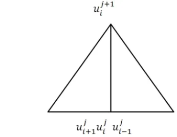
When the Explicit Scheme is used for the Burger_Fisher equation, the value of the non-defined function ui, j + 1 is specified at time tj + 1 in terms of function values defined at ui + 1, j, ui, j, ui-1, j, In Figure 1:

Figure 1. Shows the shape of the clamp used in the explicit method.

To start calculations from the first row t = t0 = 0, the solution

values are calculated from the initial condition of the problem

u x, 0 f x (6) Now take the Burger_Fisher formula of equation (1) and using the Forward Finite Difference equation and Central Finite Difference Equation (Central), Equation (1.1) is converted into a variance equation as follows:

!"#$% !"

& '

( !#$" % !)$"

* !#$

" _% ! "₊

!)$ "

* '

( ₁ ' (

(7)

'(+ '( ,&_* '( '+( ,&_* '( '%( -_*& '+( _*& '( _*& '%( . / '( / '( '( (8)

Let 0 _*&

(3)

5. Derivation of the Formula of the Exponential Scheme Method of the Equation

(Burger__Fisher)

Now the formula of the exponential differences will be derived to solve the Burger_Fisher equation as follows.

Assume that F (u) denotes any continuous and derivable function by multiplying equation (1) with a derivative F that yields to us:

3 ₄₅ _- _{1 −} _.

(10)

This leads to that

3_{= 4}₅ _- ₋ ₊ _{1 −} _.

(11)

Using the usual progressive differences and compensating for 3, found

4 _'(+ _{= 4}

'( + /45 '( '(− '( '(+ '( 1 − '( (12)

Assume that F (u) = ln (u) Produce

67 _'(+ _{= 67}

'( + &

!

" '(− '( '(+ '( 1 − '( (13)

And by taking the exp for the together Produce

'(+ = '(∗ exp &

!

" '(− '( ; '(+ '( 1 − '( < (14)

Now using the formula of the central differences by compensating in equation (1)

'(+ = '(∗ = > &

!

"? ? !#$ " _%

! "₊

!)$"

* @ − '( ? !#$

" _% !)$ "

* @ + '(@ 1 − '( (15)

Where Equation (15) is the equation used to solve using the exponential ending method.

6. Derivation of the DuFort_Frankel Formula for the Burger_Fisher Equation

This method by the world (DuFort_Frankel) in 1953 proposed a solution for the heat equation ut = uxx using the explicit

method, declaring that this method is a stable method unconditionally [11].

Now the DuFort_Frankel formula will be derived to solve the Burger_Fisher equation as follows.

Let's take the Burger_Fisher formula of equation (1) and use the equations of the Equation Difference (Central Equation) for (x) and using the central differences for time (t), equation (1) becomes a equation of differences as follows:

! "#$_%

! ")$

& = !#$

" _% !"+ !)$"

* − '( !#$

" _% !)$ "

* + '( 1 − '( (16)

According to method the (DuFort_Frankel) With compensation _'( !

"#$₊ ! ")$

!"#$% !")$

& = !

"#$ %-! "#$₊

!")$.+ !)$"

* + * − '( '+( + * '( '%( + '( 1 − '( (17)

By multiplying the ends of equation (17) in (2k) and converting _'(% to the right hand side produce

'(+ = '(% +_*& '+( − '(+ − '(% + '%( +&_* '( '%( − '+( + 2/ '( 1 − '( (18)

Assuming that 0 =_*&

1 + 20 '(+ = 1 − 20 '(% + 20 '+( + '%( + 0ℎ '( '%( − '+( + 2ℎ 0 '( 1 − '( (19)

(4)

7. Numerical Results

The Burger Fisher equation was taken in one dimension of equation (1) with the initial condition and boundary conditions of equation [4].

1 − (20)

In the interval 0 ≤ ≤ 1, ≥ 0 And the initial condition

, 0 = + tanh %,₊ G ₍₂₁₎

And boundary conditions

0, = + tanh ,₊ ,₊ +H +_, G ₍₂₂₎

1, = + tanh %,₊ 1 − ,₊ +H +_, G ₍₂₃₎

And the exact solution

, = + tanh %,₊ − ,₊ +H +_, G ₍₂₄₎

Then obtain the results shown in subsequent tables.

Table 1. The error value of the B_F equation in one dimension is illustrated using the three finite difference methods with the exact solution for interval (0.1) at time t = 0.0008 When µ = 1, β = 0.001, α = 5, I = 1.

(i, j) Absolute Error Of Explicit Method Absolute Error Of Exponential Method AbsoluteError Of DuFort_FrankelMethod

(9, 1) 0 0 0

(9, 2) 5.346351554524897e-008 1.530319240772293e-008 3.461619225986201e-008

(9, 3) 1.063982372206951e-007 3.111808165312535e-008 1.964031857981663e-008

(9, 4) 1.587900719246527e-007 4.745126878924477e-008 5.332554126047384e-008

(9, 5) 2.106254935047014e-007 6.430908744414765e-008 2.532872667160291e-008

(9, 6) 2.618915223573382e-007 8.169761385456997e-008 7.422385069066895e-008

(9, 7) 3.125757065264301e-007 9.962267565055694e-008 5.032264871474013e-008

(9, 8) 3.626661037314793e-007 1.180898601266245e-007 1.293377130673346e-007

(9, 9) 4.121512630766988e-007 1.371045230680323e-007 1.253528167932672e-007

(9, 10) 4.610202081478665e-007 1.566717966333675e-007 2.482499735084742e-007

(9, 11) 5.092624202479579e-007 1.767965972648833e-007 2.787933368469941e-007

Table 2. The error value of the B_F equation in one dimension is illustrated using the three finite differences methods with the exact solution for interval (0.1) at time t = 0.0009When µ = 1, β = 0.001, α = 5, δ =1.

(i, j) Absolute Error Of Explicit Method Absolute Error Of Exponential Method Absolute Error Of Du Fort_Frankel Method

(10, 1) 0 0 0

(10, 2) 1.109507649643682e-007 3.657658147193654e-008 2.048571144663836e-008

(10, 3) 2.201317535477365e-007 7.217126744840652e-008 8.241170747214088e-008

(10, 4) 3.275726286194880e-007 1.067982100949605e-007 9.420791101805159e-007

(10, 5) 4.333023178454409e-007 1.404712116070961e-007 1.610371151566925e-007

(10, 6) 5.373490347543308e-007 1.732037343965542e-007 1.469191355241151e-007

(10, 7) 6.397402978891575e-007 2.050089099731034e-007 1.445369626540405e-006

(10, 8) 7.405029505413996e-007 2.358995485340909e-007 2.300108626132613e-006

(10, 9) 8.396631787505049e-007 2.658881471523378e-007 4.673461453399974e-006

(10, 10) 9.372465303580935e-007 2.949868993656901e-007 6.337271046222281e-006

(10, 11) 1.033277931564158e-006 3.232077025461244e-007 9.462960673112253e-006

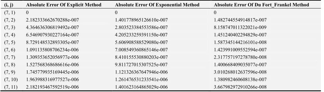
Table 3. The error value of the B_F equation in one dimension is illustrated using the three finite differences methods with the exact solution for interval (0.1) at time t = 0.0006 When µ=1, β=0.01, α=1, δ=2.

(7, 1) 0 0 0

(7, 2) 2.182333662670288e-007 1.401778965126610e-007 1.482744554914817e-007

(7, 3) 4.364636306819492e-007 2.803523384553586e-007 8.158747011322021e-009

(7, 4) 6.546907930227164e-007 4.205233259391150e-007 1.451240402294829e-007

(7, 5) 8.729148532893305e-007 5.606908588529080e-007 1.587345144216101e-008

(7, 6) 1.091135808706234e-006 7.008549360865146e-007 1.423991009552594e-007

(7, 7) 1.309353652056977e-006 8.410155530880203e-007 2.317757197278780e-008

(7, 8) 1.527568368686616e-006 9.811727015307525e-007 1.400668409035077e-007

(7, 9) 1.745779935169445e-006 1.121326367647946e-006 3.010268012637596e-008

(7, 10) 1.963988316977527e-006 1.261476531233541e-006 1.380982460608138e-007

(5)

Table 4. The error value of the B_F equation in one dimension is illustrated using the three finite differences methods with the exact solution for interval (0.1) at time t = 0.0008 When µ=1, β=0.01, α=1, δ=2.

(9, 1) 0 0 0

(9, 2) 2.457067078687203e-007 1.515046639255502e-007 1.462309786592897e-007

(9, 3) 4.914099231978497e-007 3.030058131070490e-007 8.320636846192997e-009

(9, 4) 7.370831806019496e-007 4.544878212664472e-007 1.433555391061603e-007

(9, 5) 9.827010725160790e-007 6.059356866261467e-007 1.447296826828648e-008

(9, 6) 1.228239213002524e-006 7.573350111478305e-007 1.408513496947705e-007

(9, 7) 1.473674201224462e-006 9.086719784390240e-007 2.207750859906099e-008

(9, 8) 1.718983587695178e-006 1.059933333436014e-006 1.421462273443197e-007

(9, 9) 1.964145840638309e-006 1.211106363308012e-006 3.447529173250530e-008

(9, 10) 2.209140313458313e-006 1.362178878139275e-006 1.504018364295590e-007

(9, 11) 2.453947213876262e-006 1.513139192277357e-006 5.474679409811500e-008

Figure 2. A comparison of the numerical solutions of the B_F equation in one dimension using the three finite differences methods with the solution determined in interval (0.1) at time t = 0.0008 and when 1, = 0.001, = 5, I = 1.

Figure 3. A comparison of the numerical solutions of the B_F equation in one dimension using the three finite differences methods with the solution determined in interval (0.1) at time t = 0.0009 When = 1, = 0.001, = 5, I = 1.

0 0.1 0.2 0.3 0.4 0.5 0.6 0.7 0.8 0.9 1

0.1192 0.1193 0.1194 0.1195 0.1196 0.1197 0.1198 0.1199 0.12

Comparsion Between Exact Solution and Three Numerical Method

X

T

Exact Solution Explicit Exponential DuFort - Frankel

0 0.1 0.2 0.3 0.4 0.5 0.6 0.7 0.8 0.9 1

0.0953 0.0954 0.0955 0.0956 0.0957 0.0958 0.0959 0.096

X

T

(6)

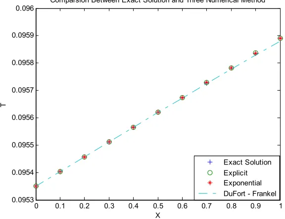
Figure 4. A comparison of the numerical solutions of the B_F equation in one dimension using the three finite differences ethods with the solution determined in interval (0.1) at time t = 0.0006 When 1, = 0.01, = 1, I = 2.

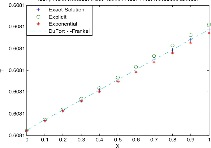
Figure 5. A comparison of the numerical solutions of the B_F equation in one dimension using the three finite differences methods with the solution determined in interval (0.1) at time t = 0.0008 When = 1, = 0.01, = 1, I = 2.

8. Conclusions

During the study of the equation B_F we noted that it is one of the important thermal equations in engineering and physical applications, and is a nonlinear equation.

Where the one-dimensional B_F equation was solved by three methods of ending difference methods and the closest

solution to the solution was found at different values of the parameters used in the equation.

When using the parameters = 1, = 0.001, = 5, I =

1 and at time t = 0.0008 we observed that the (DuFort_Frankel) method is closer to the solution determined by Table 1, and when using the parameters = 1, =

0.001, = 5, I = 1and at time t = 0.0009 Notes that the

0 0.1 0.2 0.3 0.4 0.5 0.6 0.7 0.8 0.9 1

0.6335 0.6335 0.6335 0.6335 0.6335 0.6335

X

T

Exact Solution Explicit Exponential DuFort - Frankel

0 0.1 0.2 0.3 0.4 0.5 0.6 0.7 0.8 0.9 1

0.6081 0.6081 0.6081 0.6081 0.6081 0.6081 0.6081

X

T

(7)

(exponential method) is closer to the solution determined in Table 2, and when using the parameters µ=1, β=0.01, α=1, δ=2 at time t = 0.0006 Notes that the (DuFort_Frankel) method is closer to the solution determined by Table 3, and when using the parameters µ=1, β=0.01, α=1, δ=2 at time t = 0.0008 Notes that the (DuFort_Frankel) method is the closest to the solution determined in Table 4.

References

[1] Vinay Chandraker Ashish Awasthi Simon Jayaraj, (2016) "Numerical Treatment of Burger-Fisher Equation" https://doi.org/10.1016/j.protcy.2016.08.210, Volume 25, Pages 1217-1225.

[2] Vinay Chandraker, Ashish Awasthi, Simon Jayaraj, (2016), “Numerical Treatment of Burger-Fisher equation”, Procedia Technology 25 (2016) 1217–1225.

[3] Ashok K. Singh And B. S. Bhadauria, (2009), “Finite Difference Formulae for Unequal Sub- Intervals Using Lagrange’s Interpolation Formula”, Department of Mathematics, Faculty of Science, Banaras Hindu University, Vol. 3, No. 17, pp. 815-827.

[4] M. Javidi, (2006), “Modified Pseudospectral Method For Generalized Burger’s_Fisher Equation” International Mathematical Forum, 1, No. 32, pp 1555-1564.

[5] Al-Mula, Ahmed F. K., (2005), “Stability analysis and numerical solution to Fisher Equation”, thesis master, University Mosul.

[6] Al-Naser, Shrooq, M. A., (2013), “Stability Analysis and the numericalsolution for kuramoto-sivashinsky equation”, thesis master, University Mosul.

[7] K. Pandey, Lajja Verma and Amit K. Verma, (2013), “Du Fort–Frankelfinite difference scheme for Burgers equation” Vol. 2, pp. 91-101, DOI: 10.1007/s40065-012-0050-1, published with open access at Springerlink.

[8] Jianying Zhang and Guangwu Yan, (2010), “A Lattice Boltzmann ModelFor the Burger’s_Fisher Equation”, College of Mathematics, Jilin University, Changchun 130012, People’s Republic of China.

[9] Grujic, Z., (2000), “Spatial Analyticity on the Global Attractor for the Kuramoto-Sivashinsky Equation”, J. of Dynamics and Differential Equations, Vol. 12, No. 1, PP. 217-228.

[10] Guo B. and Xiang M. X., (1997), “The Large Time Convergence of Spectral Method for Generalized kuramoto-Sivashinsky Equations”, J. of Computational Mathematics, Vol. 15, No. 1, PP. 1-13.