DOI10.1186/2190-8567-1-7
R E S E A R C H Open Access
Analysis of nonlinear noisy integrate & fire neuron
models: blow-up and steady states
María J Cáceres·José A Carrillo· Benoît Perthame
Received: 29 October 2010 / Accepted: 18 July 2011 / Published online: 18 July 2011
© 2011 Cáceres et al.; licensee Springer. This is an Open Access article distributed under the terms of the Creative Commons Attribution License
Abstract Nonlinear Noisy Leaky Integrate and Fire (NNLIF) models for neurons networks can be written as Fokker-Planck-Kolmogorov equations on the probability density of neurons, the main parameters in the model being the connectivity of the network and the noise. We analyse several aspects of the NNLIF model: the number of steady states,a prioriestimates, blow-up issues and convergence toward equilib-rium in the linear case. In particular, for excitatory networks, blow-up always occurs for initial data concentrated close to the firing potential. These results show how critical is the balance between noise and excitatory/inhibitory interactions to the con-nectivity parameter.
Keywords Leaky integrate and fire models·noise·blow-up·relaxation to steady state·neural networks
AMS Subject Classification 35K60·82C31·92B20
MJ Cáceres (
)Departamento de Matemática Aplicada, Universidad de Granada, E-18071 Granada, Spain e-mail:[email protected]
JA Carrillo
ICREA and Departament de Matemàtiques, Universitat Autònoma de Barcelona, E-08193 Bellaterra, Spain
e-mail:[email protected]
B Perthame
Laboratoire Jacques-Louis Lions, UPMC, CNRS UMR 7598 and INRIA-Bang, F-75005, Paris, France 2 - Institut Universitaire de France
1 Introduction
The classical description of the dynamics of a large set of neurons is based on de-terministic/stochastic differential systems for the excitatory-inhibitory neuron net-work [1,2]. One of the most classical models is the so-called noisy leaky integrate and fire (NLIF) model. Here, the dynamical behavior of the ensemble of neurons is encoded in a stochastic differential equation for the evolution in time of membrane potentialv(t )of a typical neuron representative of the network. The neurons relax to-wards their resting potentialVLin the absence of any interaction. All the interactions of the neuron with the network are modelled by an incoming synaptic currentI (t ). More precisely, the evolution of the membrane potential follows, see [3–8]
Cm dV
dt = −gL(V −VL)+I (t ), (1.1)
whereCmis the capacitance of the membrane andgLis the leak conductance, nor-mally taken to be constants withτm=gL/Cm≈2 ms being the typical relaxation
time of the potential towards the leak reversal (resting) potentialVL≈ −70 mV. Here,
the synaptic current takes the form of a stochastic process given by:
I (t )=JE CE
i=1
j
δt−tEji −JI CI
i=1
j
δt−tIji , (1.2)
whereδis the Dirac Delta at 0. Here,JE andJIare the strength of the synapses,CE
andCIare the total number of presynaptic neurons andtEji andtIji are the times of the
jth-spike coming from theith-presynaptic neuron for excitatory and inhibitory neu-rons respectively. The stochastic character is embedded in the distribution of the spike times of neurons. Actually, each neuron is assumed to spike according to a stationary Poisson process with constant probability of emitting a spike per unit timeν. More-over, all these processes are assumed to be independent between neurons. With these assumptions the average value of the current and its variance are given byμC=bν
withb=CEJE−CIJI andσC2=(CEJE2+CIJI2)ν. We will say that the network is average-excitatory (average-inhibitory resp.) ifb >0 (b <0 resp.).
Being the discrete Poisson processes still very difficult to analyze, many authors in the literature [3–5,7–9] have adopted the diffusion approximation where the synap-tic current is approximated by a continuous in time stochassynap-tic process of Ornstein-Uhlenbeck type with the same mean and variance as the Poissonian spike-train pro-cess. More precisely, we approximateI (t )in (1.2) as
I (t ) dt≈μcdt+σCdBt,
whereBt is the standard Brownian motion, that is,Bt are independent Gaussian pro-cesses of zero mean and unit standard deviation. We refer to the work [5] for a nice review and discussion of the diffusion approximation which becomes exact in the infinitely large network limit, if the synaptic efficaciesJE andJI are scaled
Finally, another important ingredient in the modelling comes from the fact that neurons only fire when their voltage reaches certain threshold value called the thresh-old or firing voltageVF ≈ −50 mV. Once this voltage is attained, they discharge
themselves, sending a spike signal over the network. We assume that they instanta-neously relax toward a reset value of the voltageVR≈ −60 mV. This is fundamental
for the interactions with the network that may help increase their membrane potential up to the maximum level (excitatory synapses), or decrease it for inhibitory synapses. Choosing our voltage and time units in such a way thatCm=gL=1, we can sum-marize our approximation to the stochastic differential equation model (1.1) as the evolution given by
dV =(−V+VL+μc) dt+σCdBt (1.3)
forV ≤VF with the jump process:V (to+)=VRwhenever att0the voltage achieves the threshold valueV (to−)=VF; withVL< VR< VF. Finally, we have to specify the
probability of firing per unit time of the Poissonian spike trainν. This is the so-called firing rate and it should be self-consistently computed from a fully coupled network together with some external stimuli. Therefore, the firing rate is computed asν= νext+N (t ), see [5] for instance, whereN (t )is the mean firing rate of the network. The value ofN (t )is then computed as the flux of neurons across the threshold or firing voltageVF. We finally refer to [10] for a nice brief introduction to this subject.
Coming back to the diffusion approximation in (1.3), we can write a partial dif-ferential equation for the evolution of the probability densityp(v, t )≥0 of finding neurons at a voltagev∈(−∞, VF]at a timet≥0. A heuristic argument using Ito’s
rule [3–5,7–9,11] gives the backward Kolmogorov or Fokker-Planck equation with sources
∂p ∂t(v, t )+
∂ ∂v
hv, N (t )p(v, t )−aN (t )∂
2p
∂v2(v, t ) =δ(v−VR)N (t ), v≤VF,
(1.4)
withh(v, N (t ))= −v+VL+μcanda(N )=σC2/2. We have the presence of a source term in the right-hand side due to all neurons that at timet≥0 fired, sent the signal on the network and then, their voltage was immediately reset to voltageVR. More-over, no neuron should have the firing voltage due to the instantaneous discharge of the neurons to reset valueVR, then we complement (1.4) with Dirichlet and initial
boundary conditions
p(VF, t )=0, p(−∞, t )=0, p(v,0)=p0(v)≥0. (1.5)
Equation (1.4) should be the evolution of a probability density, therefore VF
−∞p(v, t ) dv=
VF
−∞p
0(v) dv=1
N (t )as the flux of neurons at the firing rate voltage. More precisely, the mean firing rateN (t )is implicitly given by
N (t ):= −aN (t )∂p
∂v(VF, t )≥0. (1.6)
Here, the right-hand side is nonnegative since p≥0 over the interval [−∞, VF]
and thus,∂p∂v(VF, t )≤0. In particular this imposes a limitation on the growth of the functionN →a(N )such that (1.6) has a unique solutionN. Let us mention that a rigorous passage from the stochastic differential equation with jump processes (1.3) to the nonlinear equation (1.4)-(1.6) is a very interesting issue but outside the scope of this paper, see related results in which nonlinearities are nonlocal functionals in [12,
13].
The above Fokker-Planck equation has been widely used in neurosciences. Often the authors prefer to write it in an equivalent but less singular form. To avoid the Dirac delta in the right hand side, one can also set the same equation on(−∞, VR)∪ (VR, VF]and introduce the jump condition
p(VR−, t )=p(VR+, t ), ∂ ∂vp(V
−
R, t )− ∂ ∂vp(V
+
R, t )=N (t ).
This is completely transparent in our analysis which relates on a weak form that applies to both settings.
Finally, let us choose a new voltage variable by translating it with the factor
VL+bνext while, for the sake of clarity, keeping the notation for the rest of values of the potentials involvedVR< VF. In these new variables, the drift and diffusion
coefficients are of the form
h(v, N )= −v+bN, a(N )=a0+a1N, (1.7) whereb >0 for excitatory-average networks and b <0 for inhibitory-average net-works,a0>0 anda1≥0. Some results in this work can be obtained for some more general drift and diffusion coefficients. The precise assumptions will be specified on each result. Periodic solutions have been numerically reported and analysed in the case of the Fokker-Planck equation for uncoupled neurons in [14, 15]. Also, they study the stationary solutions for fully coupled networks obtaining and solving nu-merically the implicit relation that the firing rateN has to satisfy, see Section3for more details.
22], this leads to nonlinear models that exhibit naturally periodic activity and blow-up cannot happen. Nonlinear IF models are able to produce different patterns of activity and excitability types while linear models do not.
In this work we will analyse certain properties of the solutions to (1.4)-(1.5) with the nonlinear term due to the coupling of the mean firing rate given by (1.6). Next section is devoted to a finite time blow-up of weak solutions for (1.4)-(1.6). In short, we show that whenever the value ofb >0 is, we can find suitable initial data con-centrated enough at the firing rate such that the defined weak solutions do not exist for all times. We remark that, in the same sense that Brunel in [4], we use the term
asynchronousfor network states for which the firing rate tends asymptotically to con-stant in time, while we denote bysynchronousthose for which this does not happen. Therefore, a possible interpretation of the blow-up is that synchronization occurs in the model since the firing rate diverges for a fixed time creating possibly a strong par-tial synchronization, that is, a part of the network firing at the same time. Although one could also consider the blow-up as an artifact of these solutions, since neurons firing arbitrarily fast is not biologically plausible. As long as the solution exists in the sense specified in Section2, we can geta prioriestimates on theL1loc-norm of the firing rate. Section3deals with the stationary states of (1.4)-(1.6). We can show that there are unique stationary states forb≤0 anda constant but for b >0 dif-ferent cases may happen: one, two or no stationary states depending on how large
b is. In Section 4, we discuss the linear problemb=0 with a constant for which the general relative entropy principle applies implying the exponential convergence towards equilibrium. Finally by means of numerical simulations, in Section5we il-lustrate the results of previous sections about blow-up and steady states. Moreover, this numerical analysis allows us to conjecture about nonlinear stability properties of the stationary states: in case of only one steady state it is asymptotically stable and in case of two different stationary solutions the results show that the one with lower firing rate is locally asymptotically stable while the one with higher stationary firing value is either unstable or with a very small region of attraction. Our results and sim-ulations describe situations which can be identified with neuronal phenomena such as synchronization/asynchronization of a network and bistability networks. Bi- and multi-stable networks have been used, for instance in models of visual perception and decision making [23–25]. Our analysis in Sections2, 3 and5 imply that this simple model encodes complicated dynamics, in the sense that, only in terms of the connectivity parameterb, very different situations can be described with this model: blow-up, no steady state, only one steady state and several stationary states.
2 Finite time blow-up anda prioriestimates for weak solutions
Since we study a nonlinear version of the backward Kolmogorov or Fokker-Planck equation (1.4), we start with the notion of solution:
for any test function φ (v, t )∈ C∞((−∞, VF] × [0, T]) such that ∂ 2φ
∂v2, v ∂φ ∂v ∈ L∞((−∞, VF)×(0, T )),we have
T
0 VF
−∞p(v, t )
−∂φ
∂t − ∂φ
∂vh(v, N )−a ∂2φ ∂v2 dv dt =
T
0
N (t )φ (VR, t )−φ (VF, t )dt (2.1)
+ VF
−∞p
0(v)φ (
0, v) dv−
VF
−∞p(v, T )φ (T , v) dv.
Here, the notationLp(), 1≤p <∞, refers to the space of functions such that fpis integrable in, whileL∞corresponds to the space of bounded functions in. The set of infinitely differentiable functions inis denoted byC∞()used as test functions in the notion of weak solution. These non-negativity assumptions are rea-sonable. Indeed, for a givenN (t ), if we were to replaceN byN+in the right hand side of (1.4), we obtain a linear equation which solution is non-negative and (1.6) givesN≥0; that this fixed point may work is a more involved issue, since we prove that there are not always global solutions, which requires functional spaces and this motives thea prioriestimates that we derive at the end of this section.
Let us remark that the growth condition on the test function together with the assumption (1.7) imply that the term involvingh(v, N )makes sense. By choosing test functions of the formψ (t )φ (v), this formulation is equivalent to say that for all
φ (v)∈C∞((−∞, VF])such thatv∂φ∂v∈L∞((−∞, VF)), we have that
d dt
VF
−∞φ (v)p(v, t ) dv
= VF
−∞
∂φ
∂vh(v, N )+a ∂2φ
∂v2 p(v, t ) dv+N (t )
φ (VR)−φ (VF)
(2.2)
holds in the distributional sense. It is trivial to check that weak solutions conserve the mass of the initial data by choosingφ=1 in (2.2), and thus,
VF
−∞p(v, t ) dv=
VF
−∞p
0(v) dv=
1. (2.3)
The first result we show is that global-in-time weak solutions of (1.4)-(1.6) do not exist for all initial data in the case of an average-excitatory network. This result holds with less stringent hypotheses on the coefficients than in (1.7) with an analogous notion of weak solution as in Definition2.1.
Theorem 2.2(Blow-up) Assume that the drift and diffusion coefficients satisfy
h(v, N )+v≥bN and a(N )≥am>0, (2.4)
for all −∞< v≤VF and all N ≥0, and let us consider the average-excitatory network where b >0. Chooseμ >max(VF
am,
1
enough aroundv=VF,in the sense that
VF
−∞e
μvp0(v) dv
is close enough toeμVF,then there are no global-in-time weak solutions to(1.4)
-(1.6).
Proof We choose a multiplierφ (v)=eμv withμ >0 and define the number
λ=φ (VF)−φ (VR)
bμ >0
by hypotheses. For a weak solution according to (2.1), we find from (2.2) that
d dt
VF
−∞φ (v)p(v, t ) dv
≥μ
VF
−∞
bN (t )−vφ (v)p(v, t ) dv
+μ2am
VF
−∞φ (v)p(v, t ) dv−λbμN (t )
≥μ
VF
−∞φ (v)p(v, t ) dv
bN (t )+μam−VF
−λμbN (t ),
(2.5)
where (2.4) and the fact thatv∈(−∞, VF)was used. Let us now choose μlarge
enough such thatμam−VF>0 according to our hypotheses and denote
Mμ(t )=
VF
−∞φ (v)p(v, t ) dv,
which satisfies
d
dtMμ(t )≥bμN (t )
Mμ(t )−λ.
If initiallyMμ(0)≥λ and using Gronwall’s Lemma sinceN (t )≥0, we have that Mμ(t )≥λ, for allt≥0, and back to (2.5) we find
d dt
VF
−∞φ (v)p(v, t ) dv≥μ(μam−VF)
VF
−∞φ (v)p(v, t ) dv
which in turn implies, VF
−∞φ (v)p(v, t ) dv≥e
μ(μam−VF)t
VF
−∞φ (v)p
0(v) dv.
On the other hand, sincep(v, t )is a probability density, see (2.3), andμ >0 then VF
−∞φ (v)p(v, t ) dv≤e
leading to a contradiction.
It remains to show that the set of initial data satisfying the size conditionMμ(0)≥ λis not empty. To verify this, we can approximate as much as we want by smooth initial probability densities an initial Dirac mass atVF which gives the condition
eμVF≥λ=e
μVF−eμVR
bμ together withμam> VF.
This can be equivalently written as
μ≥1−e
−μ(VF−VR)
b and μ >
VF am.
Choosingμ >max(1b,VF
am), these conditions are obviously fulfilled.
As usual for this type of blow-up result similar in spirit to the classical Keller-Segel model for chemotaxis [26,27], the proof only ensures that solutions for those initial data do not exist beyond a finite maximal time of existence. It does not charac-terize the nature of the first singularity which occurs. It implies that either the decay at infinity is false, although not probable, implying that the time evolution of probability densities ceases to be tight, or the functionN (t )may become a singular measure in finite time instead of being anL1loc(R+)function. Actually, in the numerical com-putations shown in Section5, we observe a blow-up in the value of the mean firing rate in finite time. To continue the solution will need a modification of the notion of solution introduced in Definition2.1. It would be useful, since the firing rate does not become constant in time and consequently a possible interpretation is that syn-chronization occurs, a phenomena that is of interest to neuroscientists, see also the comments in the introduction and the conclusions.
Although in this paper the nature of blow-up is not mathematically identified, we devote the rest of the section to prove somea prioriestimates which shed some light on this direction. To be more precise, our estimates indicate that this blow-up should not come from a loss of mass atv≈ −∞, or a lack of fast decay rate because the second moment invis controlled uniformly in blow-up situations. We obtain these
a prioribounds with the help of appropriate choices of the test functionφin (2.1). Some of these choices are not allowed due to the growth at−∞of the test functions. We will say that a weak solution is fast-decaying at−∞if they are weak solutions in the sense of Definition2.1and the weak formulation in (2.2) holds for all test functions growing algebraically inv.
Lemma 2.3(A prioriestimates) Assume(1.7)on the drift and diffusion coefficients and that(p, N ) is a global-in-time solution of (1.4)-(1.6) in the sense of Defini-tion 2.1 fast decaying at −∞, then the following a priori estimates hold for all T >0:
(i) Ifb≥VF−VR,then
VF
−∞(VF −v)p(v, t ) dv≤max
VF,
VF
−∞(VF−v)p
0(v) dv
(b−VF+VR)
T
0
N (t ) dt≤VFT +
VF
−∞(VF−v)p
0(v) dv.
(ii) Ifb < VF −VRthen
VF
−∞(VF−v)p(v, t ) dv≥min
VF,
VF
−∞(VF −v)p
0(v) dv
.
Moreover,if in additionais constant then
T
0
N (t ) dt≤(1+T )C(VF, VR, a, p0). (2.6)
Proof Using (1.7) together with our decay assumption at−∞, we may use the test functionφ (v)=VF −v≥0. Then (2.2) gives
d
dt
VF
−∞φ (v)p(v, t ) dv
= VF
−∞
v−bN (t )p(v, t ) dv+N (t )(VF−VR).
This is also written as
d dt
VF
−∞φ (v)p(v, t ) dv+
VF
−∞φ (v)p(v, t ) dv
=VF−N (t )b−(VF−VR).
(2.7)
To prove (i), we notice that with our condition onb, the term inN (t )is nonpositive and the first result follows from Gronwall’s inequality. The second result just follows after integration in time.
To prove (ii), we first use again (2.7) and, because the term in N (t ) is non-negative, we find the first result. To obtain the second estimate (2.6), given ∈ (0, (VF −VR)/2), we can always choose a smooth truncation functionφ(v)∈C2
such that
φ(VF)=1, φ(v)=0 forv≤VR, φ(v)≥0, φ(v)≥0,
withφ(v)=0 outside the interval(VR, VR+)such that
φ(v)→ 1 VF−VR
for allv∈(VR, VF], as→0, (2.8)
theδ(V−VR)/(VF−VR). Then, equation (2.2) gives
d dt
VF
VR
φ(v)p(v, t ) dv+N (t )
= VF
VR
φ(v)−v+bN (t )p(v, t ) dv+a
VF
VR
φ(v)p(v, t ) dv.
Sinceφ(v)is positive and non-decreasing and using (2.8), we get for all 0<ε <˜ 1 there exists0small enough, such that for all 0< < 0:
VF
VR
φ(v)−v+bN (t )p(v, t ) dv
≤φ(VF)
max|VF|,|VR|
+bN (t ) (2.9)
≤(1+ ˜ε)(max(|VF|,|VR|)+bN (t ))
VF −VR
.
Due to the hypothesesb < VF −VR, for anyγ such that 0< γ <1−b/(VF−VR), we can findε˜small enough such that
0< γ <1− (1+ ˜ε)b
VF −VR.
Taking into account (2.8), (2.9), and thatp(v, t )is a probability density, we have for 0< < 0small enough
d dt
VF
VR
φ(v)p(v, t ) dv+γ N (t )≤
max(|VF|,|VR|) VF−VR
+aφL∞(VR,VF).
Choosing now=0/2 for instance, integration in time of the last inequality leads
to the desired inequality (2.6).
Corollary 2.4 Under the assumptions of Lemma 2.3 and assuming v2p0(v)∈ L1(−∞, VF)and0< b < VF−VR,then the following a priori estimates hold:
(i) If additionallyais constant,for allt≥0we have
VF
−∞v
2p(v, t ) dv≤C( 1+t ).
(ii) If additionally −bmin(VF,
VF
−∞(VF −v)p0(v) dv)+a1+bVF + VR2−VF2
2 ≤0,
then
VF
−∞v
2p(v, t ) dv≤max
a0, VF
−∞v
2p0(v, t ) dv
Proof We use again the weak formulation (2.1) withφ (v)=v2/2 as test function and get
d dt
VF
−∞
v2
2p(v, t ) dv+ VF
−∞v
2p(v, t ) dv
=bN (t )
VF
−∞vp(v, t ) dv+a
N (t )+N (t )V
2
R−V
2
F
2
=bN (t )
VF
−∞(v−VF)p(v, t ) dv+a
N (t )+N (t )
bVF +V
2
R−V
2
F
2
≤a0+N (t )
−bmin
VF,
VF
−∞(VF−v)p
0(v) dv
+a1+bVF+
VR2−VF2
2
thanks to the first statement of Lemma2.3(ii).
To prove (i), we just use the second statement of Lemma2.3(ii) valid foraconstant which tells us that the time integration of the right-hand side grows at most linearly in time and so doesVF
−∞v2p(v, t ) dv.
To prove (ii), we just use that the bracket is nonpositive and the results follows.
3 Steady states
3.1 Generalities
This section is devoted to find all smooth stationary solutions of the problem (1.4 )-(1.6) in the particular relevant case of a drift of the formh(v)=V0(N )−v. Let us search for continuous stationary solutionspof (1.4) such thatpisC1regular except possibly atV =VR where it isLipschitz. Using the definition in (2.2), we are then allowed by a direct integration by parts in the second derivative term ofpto deduce thatpsatisfies
∂ ∂v
v−V0(N )
p(v)+a(N ) ∂
∂vp(v)+N H (v−VR) =0 (3.1)
in the sense of distributions, withHbeing the Heaviside function, that is,H (u)=1 foru≥0 andH (u)=0 foru <0. Therefore, we conclude that
v−V0(N )
p+a(N )∂p
∂v+N H (v−VR)=C.
The definition ofN in (1.6) and the Dirichlet boundary condition (1.5) implyC=0 by evaluating this expression atv=VF. Using again the boundary condition (1.5), p(VF)=0, we may finally integrate again and find that
p(v)= N a(N )e
−(v−V0(N ))2
2a(N )
VF
v e
(w−V0(N ))2
2a(N ) H[w−V
which can be rewritten, using the expression of the Heaviside function, as
p(v)= N a(N )e
−(v−V0(N ))2
2a(N )
VF
max(v,VR)
e
(w−V0(N ))2
2a(N ) dw. (3.2)
Moreover, the firing rate in the stationary stateN is determined by the normalization condition (2.3), or equivalently,
a(N )
N =
VF
−∞
e−
(v−V0(N ))2
2a(N )
VF
max(v,VR)
e
(w−V0(N ))2
2a(N ) dw dv. (3.3)
Summarizing, all solutionspof the stationary problem (3.1), with the above referred regularity, are of the form given by the expression (3.2), whereN is any positive solution of the implicit equation (3.3).
Let us first comment that in the linear caseV0(N )=0 anda(N )=a0>0, we then get a unique stationary statep∞given by the Dawson function
p∞(v)=N∞ a0
e−
v2
2a0
VF
max(v,VR)
e
w2
2a0 dw, (3.4)
withN∞the normalizing constant to unit mass over the interval(−∞, VF].
The rest of this section is devoted to find conditions on the parameters of the model clarifying the number of solutions to (3.3). With this aim, it is convenient to perform a change of variables, and use new notations
z=v√−V0
a , u=
w−V0 √
a , wF=
VF −V0 √
a , wR=
VR−V0 √
a , (3.5)
where theN dependency has been avoided to simplify notation. Then, as in [3], we can rewrite the previous integral (and thus the condition for a steady state) as
⎧ ⎪ ⎪ ⎨ ⎪ ⎪ ⎩
1
N =I (N ),
I (N ):=
wF
−∞
e−z 2 2
wF
max(z,wR)
eu 2
2 du dz.
(3.6)
Another alternative form ofI (N )follows from the change of variabless=(z−u)/2 ands˜=(z+u)/2 to get
I (N )=2 0
−∞
wF+s
wR+s
e−2ss˜ds ds˜ = −
0
−∞
e−2s2 s
e−2swF −e−2swRds,
and consequently,
I (N )=
∞
0
e−s2/2 s
3.2 Case ofa(N )=a0
We are now ready to state our main result on steady states.
Theorem 3.1 Assumeh(v, N )=bN−v,a(N )=a0is constant andV0=bN. (i) Forb <0andb >0small enough there is a unique steady state to(1.4)-(1.6). (ii) Under either the condition
0< b < VF −VR, (3.8)
or the condition
0<2a0b < (VF −VR)2VR, (3.9) then there exists at least one steady state solution to(1.4)-(1.6).
(iii) If both(3.9)andb > VF−VR hold,then there are at least two steady states to
(1.4)-(1.6).
(iv) There is no steady state to(1.4)-(1.6)under the high connectivity condition
b >max2(VF −VR),2VFI (0). (3.10)
Remark 3.2 It is natural to relate the absence of steady state forblarge with blow-up of solutions.However,Theorem2.2in Section2shows this is not the only possible cause since the blow-up can happen for initial data concentrated enough aroundVF independently of the value ofb >0.See also Section5for related numerical results.
Proof Let us first study properties of the functionI (N ). To do that, we rewrite (3.7) as
I (N )=
∞
0
e−s2/2e−
sbN
√a
0 e
sVF
√a
0 −e
sVR
√a
0
s ds.
Taking the functionf (s)=e√sVFa0 −esVR√a0 and Taylor expanding up to second order
ats=0, we getf (s)−f (0)−f(0)s=f(θ )s2/2 withf (0)=0,f(0)=(VF − VR)/√a0, andθ∈(0, s). It is easy to see that
f(θ )≤max
VF2
2a0
eθ VF√a0, V
2
R
2a0
eθ VR√a0
,
for allθ∈(0, s). By distinguishing the cases based on the signs ofVF andVR, this
Taylor expansion implies that
e
sVF
√a
0 −e
sVR
√a
0
s −
VF−VR
√
a0
≤max(V 2
F, V
2
R)
2a0
se
smax(|VF|,|VR|)
√a
0
:=C0se
smax(|VF|,|VR|)
√a
0
for alls≥0. Then, a direct application of the dominated convergence theorem and continuity theorems of integrals with respect to parameters show that the function
I (N )is continuous onN on[0,∞). Moreover, the functionI (N )isC∞onNsince all their derivatives can be computed by differentiating under the integral sign by direct application of dominated convergence theorems and differentiation theorems of integrals with respect to parameters. In particular,
I(N )= −√b a0
∞
0
e−s2/2eswF −eswRds,
and for all integersk≥1,
I(k)(N )=(−1)k
b
√
a0 k ∞
0
e−s2/2sk−1eswF −eswRds.
As a consequence, we deduce:
1. Caseb <0:I (N )is an increasing strictly convex function and thus
lim
N→∞I (N )= ∞.
2. Caseb >0:I (N )is a decreasing convex function. Also, it is obvious from the previous expansion (3.11) and dominated convergence theorem that
lim
N→∞I (N )=0.
It is also useful to keep in mind that, thanks to the form ofI (N )in (3.6),
I (0)≤√2πwF(0)−wR(0)
emax(wR2(0),w2F(0))/2
=√2π(VF√−VR) a0
exp
max(VR2, VF2)
2a0
<∞.
(3.12)
Now, let us show that forb >0, we have
lim
N→∞N I (N )=
VF −VR
b . (3.13)
Using (3.11), we deduce
N I (N )−NVF√−VR a0
∞
0
e−s2/2e−
sbN
√a
0 ds
≤C0N ∞
0
se−s2/2e−
sbN
√a
0e
smax(|VF|,|VR|)
√a
0 ds.
A direct application of dominated convergence theorem shows that the right hand side converges to 0 asN → ∞sincesNexp(−sbN√
inN ands. Thus, the computation of the limit is reduced to show
lim
N→∞N
∞
0
e−s 2/2−√sbN
a0 ds=
√
a0
b . (3.14)
With this aim, we rewrite the integral in terms of the complementary error function defined as
erfc(x):=√2 π
∞
x
e−t2dt,
and then ∞
0
e−s 2/2−sbN√
a0 ds=e
b2N2
2a0
∞
0
e−(
s
√
2+
bN
√ 2a0)
2 ds=
√
π
√ 2e
b2N2
2a0 erfc
bN
√ 2a0
.
Finally, we can obtain the limit (3.14) using L’Hôpital’s rule
lim
N→∞N
∞
0
e−s 2/2−√sbN
a0 ds=
√
π
√ 2 Nlim→∞
erfc(√bN
2a0) e−
b2N2 2a0 N
=√2 lim
N→∞
−√b
2a0e −b2N2
2a0
−b2 a0e
−b2N2
2a0 − 1 N2e
−b2N2
2a0
= √
a0
b .
With this analysis of the functionI (N )we can now proof each of the statements of Theorem3.1:
Proof of (i) Let us start with the case b <0. Here, the function I (N ) is increas-ing, starting atI (0) <∞due to (3.12) and such that
lim
N→∞I (N )= ∞.
Therefore, it crosses to the function 1/Nat a single point.
Now, for the caseb >0 small, we first remark that similar dominated convergence arguments as above show that bothI (N )andI(N )are smooth functions ofb. More-over, it is simple to realize thatI (N )is a decreasing function of the parameterb. Now, choosing 0< b≤b∗< (VF−VR)/2, thenI (N )≥I∗(N )for allN≥0 whereI∗(N )
denotes the function associated to the parameterb∗. Using the limit (3.13), we can now infer the existence ofN∗>0 depending only onb∗such that
N I (N )≥N I∗(N ) >VF −VR
2b∗ >1
for allN≥N∗. Therefore, by continuity ofN I (N )there are solutions toN I (N )=1 and all possible crossings ofI (N )and 1/N are on the interval[0, N∗]. We observe
N I (N )is strictly increasing on the interval[0, N∗]and there is a unique solution to
N I (N )=1.
Proof of (ii)
Case of(3.8) The claim that there are solutions toN I (N )=1 for 0< b < VF−VR
is a direct consequence of the continuity ofI (N ), (3.12) and (3.13).
Case of(3.9) We are going to prove that I (N )≥1/N for 2a0
(VR−VF)2 < N <
VR
b ,
which concludes the existence of a steady state sinceI (0) <∞due to (3.12) implies thatI (N ) <1/N for smallN. Condition (3.9) only asserts that this interval forN is not empty. To do so, we show that
I (N )≥ (VR−VF)
2 2a0
forN∈
0,VR
b
which obviously concludes the desired inequalityI (N )≥1/N for the interval ofN
under consideration. The condition VR
b > N is equivalent towR>0, therefore, using (3.5) and the
expression forI (N )in (3.6), we deduce
I (N )≥
wF
wR
e−z 2 2
wF
max(z,wR)
eu 2
2 du dz≥
wF
wR
e−z 2 2
wF
z eu
2
2 du dz.
Sincez >0 andeu 2
2 is an increasing function foru >0, thene
u2
2 ≥e
z2
2 on[z, wF],
and we conclude
I (N )≥
wF
wR
wF
z
du dz=(VR−VF)
2 2a0
.
Proof of (iii) Under the condition (3.9), we have shown in the previous point the existence of an interval whereI (N ) > I /N. On one hand,I (0) <∞in (3.12) im-plies that I (N ) < I /N for N small and the condition b > VF −VR implies that I (N ) < I /N forN large enough due to the limit (3.13), thus there are at least two
crossings betweenI (N )and 1/N.
Proof of (iv) Under assumption (3.10) for b, it is easy to check that the following inequalities hold
I (0) <1/N forN≤2VF/b (3.15)
and
VF −VR bN−VF
< 1
We considerN such thatN > VF/b, this means thatwF <0. We use the formula
(3.7) forI (N )and write the inequalities
I (N ) < (wF −wR)
∞
0
e−s2/2eswF=(w
F −wR)ew 2
F/2
∞
0
e−(s−wF)2/2
=(wF −wR)ew 2
F/2
∞
−wF
e−s2/2≤(wF −wR)ew 2
F/2
∞
−wF
s
|wF| e−s2/2
=VF−VR
√
a0|wF|
where the mean-value theorem andwF <0 were used. Then, we conclude that
I (N ) <V√F−VR a0|wF|=
VF −VR bN−VF
, forN > VF/b.
Therefore, using Inequality (3.16):
I (N ) < 1
N, forN >2VF/b
and due to the fact thatI is decreasing and Inequality (3.15), we haveI (N ) < I (0) <
1/N, forN ≤2VF/b. In this way, we have shown that for allN,I (N ) <1/N and
consequently there is no steady state.
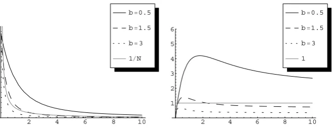
Remark 3.3 The functions I (N ) and 1/N are depicted in Figure 1 for the case V0(N )=bNanda(N )=a0illustrating the main result:steady states exist for small
b and do not exist for largeb while there is an intermediate range of existence of two stationary states.The numerical plots of the functionN I (N )might indicate that there are only three possibilities:one stationary state,two stationary states and no stationary state.However,we are not able to prove or disprove the uniqueness of a maximum for the functionN I (N )eventually giving this sharp result.
Remark 3.4 The condition (3.9) is not optimal and it can be improved by using one more term in the series expansion of the exponentials inside the integral of the expression ofI (N )in(3.7).More precisely,ifwF > wR>0,we use
eswF−eswR=
∞
n=0
sn
n!
wnF−wnR≥
2
n=0
sn
n!
wnF−wnR.
In this way,we get
I (N )≥
∞
0
e−s2/2
VF−VR
√
a0 +
1 2
wF2 −wR2s
ds
≥(VF −VR)( √
2π a0+(VF −VR)) 2a0
,
since
∞
0
e−s2/2ds=
π
2, ∞
0
e−s2/2s ds=1 and V0< VR.
Then,condition(3.9)can be improved to
2a0b < VR(VF −VR)
2π a0+(VF −VR)
.
Of course,this last inequality is not optimal either for the same reason as before.
3.3 Case ofa(N )=a0+a1N
We now treat the case ofa(N )=a0+a1N, witha0, a1>0 withb >0. Proceeding as above we can obtain from (3.7) the expression of its derivative
I(N )= − d dN
V0(N ) √
a(N ) I1(N )−I2(N )
+ d
dN
1 √
a(N )
VFI1(N )−VRI2(N )
,
(3.17)
where
I1(N )= ∞
0
e−s2/2eswFds and I
2(N )= ∞
0
e−s2/2eswRds.
ThereforeI (N )is decreasing since
d dN
V0(N ) √
a(N ) =
2ba0+ba1N 2(a0+a1N )3/2
>0 and
d dN
1 √
a(N )
= − a1
(a0+a1N )3/2
Moreover, we can check that the computation of the limit (3.13) still holds. Actually, we have
lim
N→∞
N I (N ) VF−VR =
lim
N→∞ N
√
a
∞
0
e−s2/2e−sbN /√ads= lim
N→∞
√
π
erfc(√bN
2a) e−b
2N2 2a N
√
2a
= lim
α→∞
√
πerfc(bα) e−b2α2
α
= lim
α→∞
√
π −
2
√
πbe− b2α2
−2b2α2e−b2α2−e−b2α2
α2
=1
b,
where we have used the changeα=√N
2a and L’Hôpital’s rule. In the caseb <0, we
can observe again by the same proof as before thatI (N )→ ∞whenN→ ∞, and thus, by continuity there is at least one solution toN I (N )=1. Nevertheless, it seems difficult to clarify perfectly the number of solutions due to the competing monotone functions in (3.17).
The generalization of part of Theorem3.1is contained in the following result. We will skip its proof since it essentially follows the same steps as before with the new ingredients just mentioned.
Corollary 3.5 Assumeh(v, N )=bN−v,a(N )=a0+a1Nwitha0, a1>0. (i) Under either the conditionb < VF −VR,or the conditionsb >0and 2a0b+
2a1VR< (VF −VR)2VR,then there exists at least one steady state solution to (1.4)-(1.6).
(ii) If both2a0b+2a1VR< (VF−VR)2VRandb > VF −VR hold,then there are at least two steady states to(1.4)-(1.6).
(iii) There is no steady state to(1.4)-(1.6)forb >max(2(VF−VR),2VFI (0)).
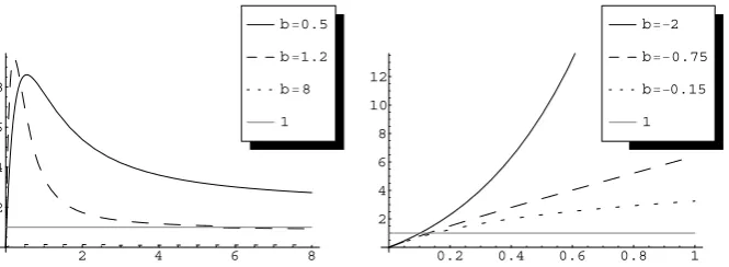
These behaviours are depicted in Figure2. Let us point out that ifa is linear and
b <0,I (N )has not to be strictly increasing as in the constant diffusion case and it may have a minimum forN >0.
At this point, a natural question is what happens with the stability of these steady states. In the next section we study it in the linear case, when the model presents only one steady state. An extension of the same techniques, entropy methods, to the nonlinear case is not straightforward at all. However, the results obtained in the linear case let us expect that for small connectivity parameterbthe only steady state could be stable. On the other hand, numerical results presented in Section5 give some numerical evidence of the stability/instability in different situations described by this model: only one steady state or two steady states, see that section for details.
4 Linear equation and relaxation
We study specifically the case of a linear equation that isb=0 anda(N )=a0, that is,
⎧ ⎪ ⎪ ⎪ ⎪ ⎪ ⎪ ⎨ ⎪ ⎪ ⎪ ⎪ ⎪ ⎪ ⎩
∂p(v, t )
∂t −
∂ ∂v
vp(v, t )−a0
∂2
∂v2p(v, t )=δ(v−VR)N (t ), v≤VF,
p(VF, t )=0, N (t ):= −a0
∂
∂vp(VF, t )≥0, a0>0, p(v,0)=p0(v)≥0,
VF
−∞p
0(v) dv=1.
(4.1)
For later purposes, we remind that the steady statep∞(v)given in (3.4) satisfies, for the case at hand, the equation
⎧ ⎪ ⎪ ⎪ ⎪ ⎪ ⎪ ⎨ ⎪ ⎪ ⎪ ⎪ ⎪ ⎪ ⎩
−∂
∂v[vp∞(v)] −a0 ∂2
∂v2p∞(v)=δ(v−VR)N∞, v≤VF,
p∞(VF)=0, N∞:= −a0
∂
∂vp∞(VF)≥0,
VF
−∞p∞(v) dv=1.
(4.2)
We will assume in this section that the initial data satisfies, for someC0>0,
p0(v)≤C0p∞(v). (4.3)
Then, we take for granted that solutions of the linear problem exist, with the regularity needed in each result below and such that for allt≥0,
p(v, t )≤C0p∞(v). (4.4)
We prove that the solutions to (4.1) converge in large times to the unique steady statep∞(v).
Theorem 4.1(Exponential decay) Fast-decaying solutions to the equation(4.1) ver-ifying(4.4)satisfy
VF
−∞p∞(v)
p(v, t )−p∞(v) p∞(v)
2
dv≤e−2a0νt
VF
−∞p∞(v)
p0(v)−p∞(v) p∞(v)
2
dv.
This result shows that no synchronization of neuronal activity can be expected when the network is not connected, since solutions tend to produce a constant firing rate, a very intuitive conclusion. Because the rate of decay is exponential, we also expect that small connectivity cannot create synchronization either, again an intuitive conclusion proved rigorously for the elapsed time structured model in [22]. Also the proof shows that two relaxation processes are involved in this effect: dissipation by the diffusion term and dissipation by the firing term. These relaxation effects are stated in the following theorem which also gives the natural bounds for the solutions to equation (4.1) (choosingG(u)=u2gives the natural energy space of the system, a weightedL2space).
Theorem 4.2(Relative entropy inequality) Fast-decaying solutions to equation(4.1)
verifying(4.4)satisfy,for any smooth convex functionG:R+−→R,the inequality
d dt
VF
−∞p∞(v)G
p(v, t ) p∞(v)
dv= −DG[p](t )≤0, (4.5)
with
DG[p](t )=N∞
G
N (t ) N∞
−G
p(v, t ) p∞(v)
−
N (t ) N∞ −
p(v, t ) p∞(v)
G
p(v, t ) p∞(v) V
R
+a0 VF
−∞p∞(v)G
p(v, t )
p∞(v)
∂ ∂v
p(v, t ) p∞(v)
2
dv≥0.
Proof of Theorem4.1 The proof is standard in Fokker-Planck theory and follows by applying the relative entropy inequality (4.5) withG(x)=(x−1)2. Then, we obtain
d dt
VF
−∞p∞(v)
p(v, t ) p∞(v)−1
2
dv≤ −2a0 VF
−∞p∞(v)
∂ ∂v
p(v, t ) p∞(v)−1
2
dv.
Proposition 4.3 There existsν >0such that
ν
VF
−∞p∞(v)
q(v) p∞(v)
2
dv≤
VF
−∞p∞(v)
∂ ∂v
q(v) p∞(v)
2
dv
for all functionsqsuch pq
∞ ∈H 1(p
∞(v) dv)andVF
−∞q(v) dv=0.
Poincaré’s-like inequality in Proposition4.3applied toq=p−p∞ bounds the right hand side on (4.6)
d dt
VF
−∞p∞(v)
p(v, t ) p∞(v)−1
2
dv≤ −2a0ν VF
−∞p∞(v)
p(v, t ) p∞(v)−1
2
dv.
Finally, the Gronwall lemma directly gives the result.
To show Theorem4.2, which was used in the proof of Theorem4.1, we need the following preliminary computations.
Lemma 4.4 Givenpa fast-decaying solution of (4.1)verifying(4.4),p∞given by
(3.4)andGaC2convex function,then the following relations hold:
∂ ∂t
p p∞−
v+2a0 p∞
∂ ∂vp∞
∂ ∂v
p p∞−a0
∂2 ∂v2
p p∞
=N∞
p∞δ(v−VR)
N N∞−
p p∞ , (4.7) ∂ ∂tG p p∞ −
v+2a0 p∞
∂ ∂vp∞
∂ ∂vG p p∞ −a0
∂2 ∂v2G
p p∞
= −a0G p p∞ ∂ ∂v p p∞ 2 +N∞
p∞δ(v−VR)
N N∞−
p p∞ G p p∞ , (4.8) ∂ ∂tp∞G
p p∞ − ∂ ∂v
vp∞G
p
p∞ −a0 ∂2 ∂v2
p∞G
p p∞
= −a0p∞G p p∞ ∂ ∂v p p∞ 2 (4.9)
+N∞δ(v−VR)
N N∞−
p p∞ G p p∞ +G p
p∞ .
Proof Since∂v∂ (pp
∞)= 1 p∞ ∂p ∂v− p p2 ∞ ∂p∞
∂v we obtain
∂p ∂v =p∞
and
∂2p ∂v2 =p∞
∂2 ∂v2 p p∞ +2 ∂
∂v p p∞ ∂p∞ ∂v + p p∞
∂2p∞ ∂v2 . Using these two expressions in
∂ ∂t p p∞ = 1 p∞ ∂p ∂t = 1 p∞
δ(v=VR)N (t )+ ∂ ∂v
vp(v, t )+a0
∂2 ∂v2p(v, t )
we obtain (4.7).
Equation (4.8) is a consequence of Equation (4.7) and the following expressions for the partial derivatives ofG(pp
∞): ∂ ∂tG p p∞ =G p p∞ ∂ ∂t p p∞ , ∂ ∂vG p p∞ =G p p∞ ∂ ∂v p p∞ and ∂2 ∂v2G
p p∞ =G p p∞ ∂ ∂v p p∞ 2 +G p p∞ ∂2 ∂v2 p p∞ .
Finally, Equation (4.9) is obtained using Equation (4.8) and the fact thatp∞is
solu-tion of (4.2).
Proof of Theorem4.2 We integrate from−∞toVF−αin (4.9) and letαtend to 0+
and use L’Hôpital’s rule
lim
v→VF
p(v, t )
p∞(v)=vlim→VF
∂p ∂v(v, t )
∂p∞ ∂v (v)
=N (t )
N∞. (4.10)
Sincep(v, t )≤C0p∞(v), then
d
dt
VF
−∞p∞G
p
p∞
dv−a0
∂
∂v
p∞G
p
p∞ V
F
= −a0 VF
−∞p∞G
p p∞ ∂ ∂v p p∞ 2 dv
+N∞
N N∞−
p p∞ G p p∞ +G p p∞ V
R
.
The Dirichlet boundary condition (1.5) implies that
−a0
∂ ∂v
p∞G
p p∞ V
F
= −a0
∂p∞ ∂v G p p∞ VF
=N∞G
N (t ) N∞
where we used that
p∞ ∂ ∂vG
p p∞
VF
=p∞G
p p∞
−
Np∞+N∞p p2
∞a0
VF
=G
p p∞
−N
a0 +
N∞ a0
p p∞
VF
=0,
due to (4.10). Collecting all terms leads to the desired inequality.
Let us finally remark that as a usual consequence of the General Relative Entropy principle (GRE) [29], the estimate (4.4) follows by choosing the convex function
G(x)=(x−C0)4+. This shows that the bound (4.4) can be proved using (4.3) together with a well-posedness theory of classical fast-decaying at−∞solutions to (4.1).
5 Numerical results
We consider two different explicit methods to simulate the NNLIF (1.4). The first one is based on standard shock-capturing methods for the advection term and standard centered finite differences for the second-order term. More precisely, the first order term is approximated by finite difference WENO-schemes [30].
The second numerical method is based on another finite difference scheme for the Fokker-Planck equation proposed in the literature called the Chang-Cooper method [31]. This method was also used in [20] for a computational neuroscience model with variable voltage and conductance. In order to use this method, the first step is to rewrite the Fokker-Planck equation (1.4) in terms of the Maxwellian
M(v)=e−(v−bN ) 2
2a(N ) as follows,
∂p
∂t(v, t )−a
N (t ) ∂ ∂v
M(v, t ) ∂ ∂v
p(v, t )
M(v, t ) =N (t )δ(v−VR).
Then, the Chang-Cooper method performs a kind ofθ-finite difference approximation ofp/M, see [31] for details. The Chang-Cooper method presents difficulties when the firing rate becomes large and the diffusion coefficienta(N )is constant. More pre-cisely, givena(N )=a0andb >0, ifNis large, the drift of the Maxwellian, in terms of which is rewritten the Fokker-Planck equation, practically vanishes on the interval
(−∞, VF]and this particular Chang-Cooper method is not suitable. Whenevera(N )
is not constant, this problem disappears.
Summarizing, we consider two different schemes for our simulations: the first one is based on WENO-finite differences as described above, and the second one by means of the cited Chang-Cooper method. In both cases the evolution on time is performed with a TVD Runge-Kutta scheme. In Section 2 of [20] these schemes are explained in details and we refer to [30,31] for a deeper analysis of them.
In our simulations we consider a uniform mesh in v, for v∈ [Vmin, VF]. The
two different types of functions: • Maxwellians:
p0(v)=√1
2π σ0
e−
(v−v0)2
2σ02 , (5.1)
where the meanv0and the varianceσ02are chosen according to the analyzed phe-nomenon.
• Stationary Profiles (3.2) given by
p(v)= N a(N )e
−(v−V0(N ))2
2a(N )
VF
max(v,VR)
e
(w−V0(N ))2
2a(N ) dw,
withN an approximate value of the stationary firing rate. We typically consider this kind of initial data to analyze local stability of steady states.
Steady states. -As we show in Section3, forbpositive there is a range of values for which there are either one or two or no steady states. With our simulations we can observe all the cases represented in Figures1and2.
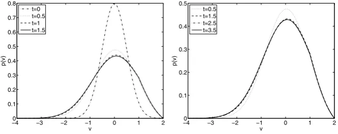
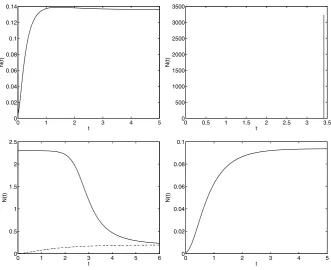
In Figure3 we show the time evolution of the distribution function p(v, t ), in the case ofa≡1 andb=0.5 for which there is only one steady state according to Theorem3.1, considering as initial data a Maxwellian withv0=0 andσ02=0.25 in (5.1). We observe that the solution after 3.5 time units numerically achieves the steady state with the imposed tolerance. The top left subplot in Figure4describes the time evolution of the firing rate, which becomes constant after some time. This clearly corresponds to the case of a unique locally asymptotically stable stationary state. Let us remark that in the right subplot of Figure3, we can observe the Lipschitz behavior of the function atVR as it should be from the jump in the flux and thus on
the derivative of the solutions and the stationary states, see Section3.
Forb=1.5, we proved in Section 3that there are two steady states. With our simulations we can conjecture that the steady state with larger firing rate is unstable. However the stationary solution with low firing rate is locally asymptotically stable. We illustrate this situation in the bottom left subplot in Figure 4. Starting with a
Fig. 4 Firing ratesN (t )fora≡1. Top left:b=0.5 with initial data a Maxwellian with:v0=0 and
σo2=0.25. Top right:b=3 with initial data a Maxwellian with:v0= −1 andσo2=0.5. Bottom left:
b=1.5 considering two different initial data: a Maxwellian with:v0= −1 andσo2=0.5 and a profile given by the expression (3.2) withN=2.31901. Bottom right:b= −1.5 with initial data a Maxwellian with:v0= −1 andσo2=0.5. The top right case seems to depict a blow-up phenomena demonstrated in Theorem2.2.
firing rate close to the high stationary firing value, the solution tends to the low firing stationary value.
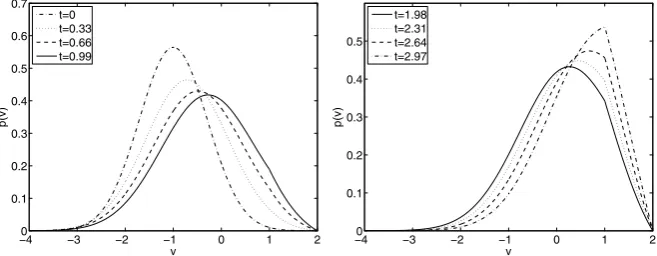
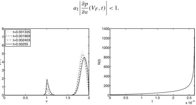
In Figure5we analyze in more details the behavior of the steady state with larger firing rate. The left subplot presents the evolution on time of the firing rate for dif-ferent distribution function starting with profiles given by the expression (3.2) with
Nan approximate value of the stationary firing rate. We show that, depending of the initial firing rate considered, its behavior is different: tends to the lower steady state or goes to infinity. The firing rate for the solution with initialN0=2.31901 remains almost constant for a period of time. Observe in Figure5that the difference between the initial data and the distribution function at timet=1.8 is almost negligible. How-ever, the system evolves slowly and att=6 the distribution is very close to the the lower steady state, see the bottom left subplot in Figure4.
In the bottom right subplot of Figure4 we observe the evolution for a negative value ofb, where we know that there is always a unique steady state, and its local asymptotic stability seems clear from the numerical experiments.