M E T H O D O L O G Y
Open Access
Bayesian reference analysis for exponential
power regression models
Marco AR Ferreira
1*and Esther Salazar
2*Correspondence: [email protected]
1Department of Statistics, University of Missouri, Columbia, USA Full list of author information is available at the end of the article
Abstract
We develop Bayesian reference analyses for linear regression models when the errors follow an exponential power distribution. Specifically, we obtain explicit expressions for reference priors for all the six possible orderings of the model parameters and show that, associated with these six parameters orderings, there are only two reference priors. Further, we show that both of these reference priors lead to proper posterior distributions. Furthermore, we show that the proposed reference Bayesian analyses compare favorably to an analysis based on a competing noninformative prior. Finally, we illustrate these Bayesian reference analyses for exponential power regression models with applications to two datasets. The first application analyzes per capita spending in public schools in the United States. The second application studies the relationship between sold home videos versus profits at the box office.
MSC: 62F15; 62F35; 62J05
Keywords: Bayesian inference; Exponential power errors; Frequentist properties; Reference prior; Robustness
1 Introduction
A flexible way to deal with outliers in linear regression is to assume that the errors fol-low an exponential power (EP) distribution. Specifically, assuming an EP distribution decreases the influence of outliers and, as a result, increases the robustness of the analysis (Box and Tiao 1962; Liang et al. 2007; Salazar et al. 2012; West 1984). In addition, the EP distribution includes the Gaussian distribution as a particular case. Further, the EP distri-bution may have tails either lighter (platykurtic) or heavier (leptokurtic) than Gaussian. Platykurtic distributions may be a result of truncation, whereas leptokurtic distributions provide protection against outliers. Salazar et al. (2012) have developed three types of Jeffreys priors for linear regression models with independent EP errors. Unfortunately, two of those priors lead to useless improper posterior distributions and only one leads to a proper posterior distribution. Here we develop explicit expressions for reference priors for all the six possible orderings of the model parameters.
We show that the six parameters orderings lead to two distinct reference priors. The parameter ordering corresponds to the order of importance of each parameter in the anal-ysis, with the most important parameter appearing first and the least important appearing last (Berger and Bernardo 1992a,b). In addition to the two formally obtained reference priors, we propose an approximate reference prior that shares the same tail behavior
but is much more straightforward to implement in practice. Finally, we show that the two reference priors lead to useful proper posterior distributions.
To make sure that Bayesian reference procedures do not bias the data analysis in an undesirable manner, it is important to study their frequentist properties. To study the frequentist properties of our proposed procedures, we have performed a Monte Carlo study that shows that our proposed Bayesian reference approaches compare favorably to a posterior analysis based on a competing prior in terms of coverage of credible inter-vals, relative mean squared error, and mean length of credible intervals. While the relative mean squared error and the mean length of credible intervals should be judged in com-parison with those yielded by competing priors, the coverage of credible intervals should be as close as possible to the nominal level.
Coverage of credible intervals close to nominal provides a guarantee of level of perfor-mance of the procedure when used automatically and independently by many researchers in their problems. In our Monte Carlo study, we have found that the Bayesian reference credible intervals that we have obtained have frequentist coverage close to nominal. These good frequentist properties results agree with previous literature on Bayesian reference analyses for other models such as, for example, Gaussian random fields (Berger et al. 2001), Markov random fields (Ferreira and De Oliveira 2007), multivariate normal mod-els (Sun and Berger 2007), and elapsed times in continuous-time Markov chains (Ferreira and Suchard 2008).
The EP density is given by
f(y|μ,σp,p)=
2p1/pσp(1+1/p)
−1
exp−pσpp
−1
|y−μ|p, −∞<y<∞, (1)
wherep>1,−∞< μ <∞andσp> 0. The EP distribution has three parameters: the
location parameterμ = E(y), the scale parameterσp =[E(|y−μ|p)]1/p, and the shape
parameterp. The scale parameterσpcan be seen as a variability index that generalizes the
standard deviation. Moreover,σp is also known as power deviation of orderp(Vianelli
1963). In addition, the kurtosis isκ =(1/p)(5/p)/((3/p))2, implying that the shape parameterpdetermines the thickness of the tails of the EP density. Specifically, the EP distribution is leptokurtic ifp < 2 (κ > 3) and platykurtic ifp > 2 (κ < 3). Finally, the EP distribution has several important especial cases such as the Laplace distribution (p=1), the normal distribution (p=2) and, whenp→ ∞, the uniform distribution on the interval(μ−σp,μ+σp)(e.g., see Box and Tiao 1992).
The remainder of the paper is organized as follows. Section 2 presents the linear model with exponential power errors and the associated likelihood function. Section 3 derives the two reference priors and shows that both of these priors lead to proper posterior dis-tributions. Section 4.1 presents a simulation study of the frequentist properties of the reference-priors-based Bayesian procedures and those of a competing noninformative prior. Section 4.2 presents applications of Bayesian reference analysis to two datasets. Section 5 concludes with a discussion of major findings and possible future research directions.
2 EP linear model
Lety=(y1,. . .,yn)be the vector of observations andx=(x1,. . .,xn)be then×kdesign
matrix of explanatory variables. We consider the linear model
y=xβ+, (2)
whereβ = (β1,. . .,βk) ∈Rkis a vector of regression coefficients, and =(1,. . .,n)
is a vector of errors such that 1,. . .,n are independent and identically distributed
and follow the exponential power distribution with location parameter equal to zero, scale parameterσp, and shape parameter p. We reparameterize the model by defining σ = p1/pσ
p(1 +1/p). This reparametrization has also been considered by Zhu and
Zinde-Walsh (2009) and Salazar et al. (2012). Let us denote the parameter vector by θ = (β,σ,p) ∈ Rk ×(0,∞)×(1,∞). Then, the log-likelihood function for the model given in Equation (2) is
l(θ;y,x) = −nlog 2−nlogσ−
n
i=1
(1+1/p)|yi−xiβ| σ
p
. (3)
We use the log-likelihood function to develop reference priors for the EP regression model.
3 Methods
In this section, we obtain explicit expressions for reference priors for all the six possible orderings of the parameters of the EP linear model, and show that associated with these six parameters orderings there are only two reference priors. Finally, we show that both of these reference priors lead to proper posterior distributions.
Specifically, we consider here the Bernardo reference priors (Bernardo 1979) that take into account the Kulback-Leibler divergency between the prior distribution and the pos-terior distribution. In a nutshell, the reference priors proposed by Bernardo maximize the expected value of perfect information about the model parameters (p. 300, Bernardo and Smith 1994). When the parameter space is one-dimensional and asymptotic normality of the posterior distribution holds, the reference prior coincides with Jeffreys prior (Jeffreys 1961). However, when the parameter space is multidimensional Jeffreys prior is known to lead to Bayesian procedures that may have undesirable frequentist properties, such as for example frequentist coverage of credible intervals far away from the desired nominal level.
(1979) suggested an approach in three stages. The first stage obtains the conditional dis-tribution of the nuisance parameter conditional on the parameter of interest. The second stage integrates out the nuisance parameter with respect to that conditional distribu-tion to obtain a marginal likelihood. Finally, the third stage applies the reference prior approach to the marginal likelihood to obtain the reference prior for the parameter of interest. This idea can be naturally extended to partitions of the parameter vector with more than two components. The resulting reference prior will then depend on the order-ing of the parameter vector components. This multiparameter case has been developed in a series of papers by Berger and Bernardo (1992a,b,c). Here we use the Berger-Bernardo approach to develop reference priors for the parameters of the EP regression model.
As we show below, the reference priors obtained here are of the form
π(θ)∝ π(σpa), (4)
wherea∈Ris a hyperparameter andπ(p)is the ‘marginal’ prior of the shape parameter
p. As shown by Salazar et al. (2012), the Jeffreys-rule prior and two independence Jeffreys priors also have the functional form (4). Specifically, using the same notation as in Salazar et al. (2012), the two independence Jeffreys priors havea= 1 and their marginal priors forpare respectively given by
πI1(p)∝p−11+p−1 1+p−1−11/2, (5)
and
πI2(p)∝p−3/21+p−1 1+p−11/2. (6)
Meanwhile, the Jeffreys-rule prior is such thata=k+1 and its marginal prior forpis
πJ(p)∝p−12−p−1k/2πI1(p). (7)
In what follows we find that the reference priors for the EP regression model are related to the independence Jeffreys priors given in Equations (5) and (6). When developing noninformative priors, it is crucial to study whether the resulting posterior distribution is proper. Salazar et al. (2012) have shown that the Independence Jeffreys priorπI2(p) yields a proper posterior distribution. Unfortunately, both the independence Jeffreys prior πI1(p)and the Jeffreys-rule priorπJ(p)yield improper posterior distributions.
The Berger-Bernardo approach to develop reference priors requires the Fisher infor-mation matrix. Specifically, for the EP regression model the Fisher inforinfor-mation matrix
H(θ), with elementsφijgiven byφij=Ey|θ −∂θ∂i∂θ2
jl(θ;y,x)
withφij=φjiandθjthe jth
element ofθ =(β,σ,p), is:
H(θ)= ⎡ ⎢ ⎣
σ−2(p−1)(2−p−1)ni=1xixi 0 0
0 npσ−2 −nσ−1p−1
0 −nσ−1p−1 np−31+p−1 1+p−1 ⎤ ⎥ ⎦,
(8)
where (α) ≡ (α)/ (α) and (α) ≡ ∂ (α)/∂α are the digamma and trigamma functions, respectively.
ordering of the groups only with respect to whetherσ orpappears first in the ordering. The following theorem provides reference priors for the parameters of the EP regression model.
Theorem 1. Consider the EP regression model with log-likelihood function given in Equation (3). Then, there are two reference priors for all six possible orderings of the model parameters. Moreover, these two reference priors are of the form (4) with a = 1. For the orderings(β,σ,p),(σ,β,p), and(σ,p,β)the ‘marginal’ reference prior for p is
πr1(p)∝p−3/21+p−1 1+p−11/2, (9)
whereas for the orderings(β,p,σ),(p,β,σ), and(p,σ,β)the ‘marginal’ reference prior for p is
πr2(p)∝p−3/21+p−1 1+p−1−11/2. (10)
Proof.See the Appendix.
While reference priorπr2 is a new prior that has not appeared before in the literature, there are similarities between the reference priors given in Theorem 1 and the indepen-dence Jeffreys priors given in Equations (5) and (6). Reference priorπr1coincides with the independence Jeffreys priorπI2 given in Equation (6). Moreover, it is important to point out that reference priorπr2 is somewhat similar to the independence Jeffreys priorπI1 given in Equation (5), differing only by a factor ofp−1/2. However, as we show below this difference betweenπI1andπr2 is enough to makeπI1yield a useless improper posterior distribution while the reference priorπr2yields a useful proper posterior distribution.
Consider a prior of the form (4). Then the integrated likelihood forpis given by
LI(p;y) ∝
Rk
∞
0
L(β,σ,p;y)σ−adσdβ.
Then the prior leads to a proper posterior distribution if and only if
∞
1
LI(p;y)π(p)dp<∞, (11)
Thus, in order to determine whether a prior of the form (4) leads to a proper posterior distribution, one needs to investigate the tail behavior of both the marginal prior and the integrated likelihood forp. The tail behavior of the marginal reference priors forpgiven in Theorem 1 is given in the following lemma.
Lemma 1. The marginal priors for p given in Theorem 1 are continuous functions in[1,∞)
and are such thatπr1(p)=Op−3/2andπr2(p)=Op−3/2as p→ ∞.
Proof.Direct inspection shows that πr1(p) and πr2(p) are continuous functions in [1,∞). Their tail behavior whenp→ ∞follows from the fact that 1+p−1→1.6449 andp−1=O(p)asp→ ∞.
Definition 1. We define an approximate reference priorπr3 to be of the form (4) with a=1and marginal prior for p equal toπr3(p)∝p−3/2.
Computation of priorπr3is faster and more straightforward than that of priorsπr1and πr2. In addition, Section 4.1 shows that the frequentist properties of procedures based onπr3 are similar to those based onπr1 andπr2. As a consequence, the approximate reference prior πr3 may become more widely used than the reference priors πr1 and πr2. Therefore, henceforth we drop the term “approximate” and simply refer toπr3 as a reference prior.
The following lemma, that was proved by Salazar et al. (2012), provides the tail behavior for the integrated likelihood forp.
Lemma 2(Salazar et al.2012). Provided that n>k+1−a, the integrated likelihood for p under the class of priors (4) is a continuous function in[1,∞)and is such that LI(p;y)= O(1)as p→ ∞.
The following proposition establishes that the two reference priors that we have obtained yield proper posterior distributions.
Proposition 1. Provided that n>k+1−a, the two reference priorsπr1andπr2given in Theorem 1 yield proper posterior distributions.
Proof.This proposition follows directly from condition (11), and Lemmas 1 and 2.
To implement posterior analysis for the parameters of the EP regression model based on the reference priors developed here, we use an approach proposed by Salazar et al. (2012) that combines Laplace approximations and Newton-Cotes integration.
4 Results and discussion
4.1 Frequentist properties
In this section we perform a simulation study to access the frequentist properties of Bayesian procedures based on the reference priorsπr1,πr2, andπr3. In addition, we com-pare the performance of these reference priors to that of a competing noninformative priorπUthat takes the form (4) witha=1 andπU(p)∝1 for 1<p<10 andπU(p)=0 otherwise. The joint priorπU(θ)leads to a proper posterior distribution, however as we see below the uniform priorπU(p)is a naïve way to express lack of information about
p. The Bayesian procedures we consider are the posterior modes and posterior medians for point estimation, and the 95% highest posterior density (HPD) credible intervals for interval estimation. Finally, we consider three frequentist measures of quality. For evaluat-ing the quality of point estimation, we consider the square root of the frequentist relative mean squared error. For evaluating the performance of interval estimation, we consider two frequentist measures: the frequentist coverage and the mean length of the credible intervals.
Finally, for each combination of parameter values and sample sizes, we have simulated 1,500 datasets to estimate the frequentist properties of the several procedures.
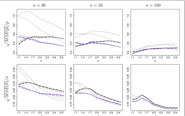
The square root of the relative mean squared error (RMSE),MSE(θ)/θ, for estimators ofpandσis shown as a function ofpin Figure 1. As intuitively expected, for all priors and for both posterior mode and median, as the sample size increases the RMSE decreases. The most substantial differences are between the performances of the posterior mode and posterior median, and between the performances of the reference priors when com-pared with theπUprior. First, we compare the performance of the posterior median and the posterior mode. For each prior, for the estimation ofp, the posterior median provides smaller RMSE than the posterior mode for most values ofpconsidered except forpclose to one. And this advantage of the posterior mode becomes less pronounced as the sam-ple size increases. For each prior, for the estimation ofσ, the posterior median provides smaller RMSE than the posterior mode. Therefore, for the reference analysis of the EP regression model we recommend the use of the posterior median.
Second, we compare the RMSE performance of the different priors. For each type of point estimator considered here, in terms of RMSE the reference priors πr1, πr2, and πr3provide qualitatively similar results, withπr1 andπr3being slightly better for smaller values ofpandπr2being slightly better for larger values ofp. In addition, the difference in performance of the three reference priors becomes smaller as the sample size increases. In contrast, the performance of the reference priors differs dramatically from that of theπU prior. For each class of estimators ofpand for all values ofpconsidered, when compared to theπU prior the reference priors lead to smaller RMSE. For the estimation ofσ, the results are mixed; for small sample sizes while the reference priors lead to smaller RMSE whenpis small and πU leads to better results whenpis larger. But for larger sample
sizes the reference priors-based posterior medians have smaller RMSE for all considered values ofp.
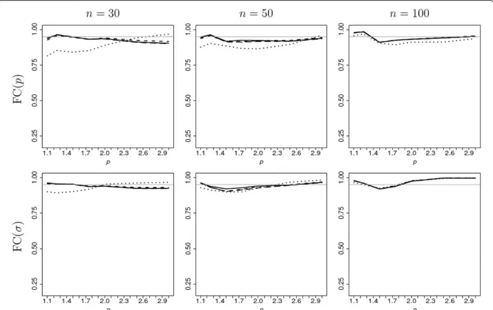
The frequentist coverage (FC) of 95% HPD credible intervals forpandσ is shown, as a function ofp, in Figure 2. As the sample size increases, the FC of the credible intervals based on the four priors becomes more similar. For both parameters, theπr1-,πr2-, and πr3-based credible intervals have frequentist coverage closer to the nominal level. This superiority of the Bayesian reference analysis is particularly pronounced for sample sizes equal to 30 or 50 and whenp<2.
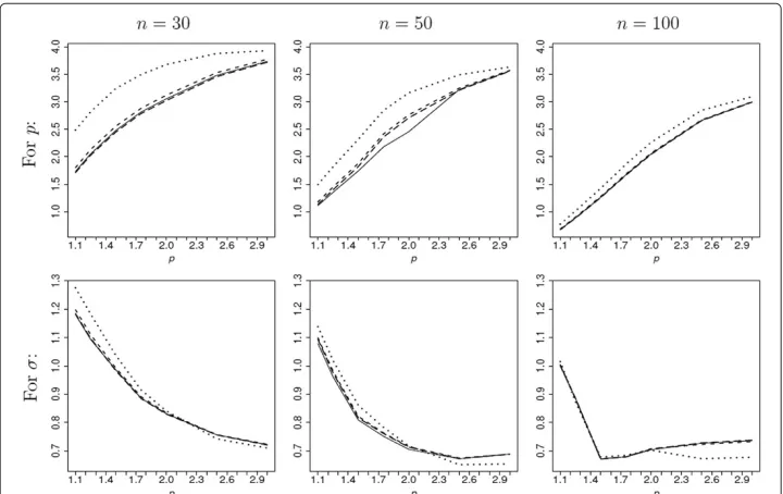
The mean length of the 95% HDP credible intervals forpandσ is shown, as a function ofp, in Figure 3. For the credible intervals based on the three reference priors, the mean lengths of the credible intervals are similar with slightly better results forπr1. For interval estimation forσ, the mean lengths of the credible intervals based on the three reference priors are smaller than the mean lengths of the credible intervals based on theπU when p < 2 and are larger when p > 2. For interval estimation ofp, in the range of values that we consider theπr1-,πr2-, andπr3-based credible intervals are on average shorter that those based onπU. Therefore, for the interval estimation ofp, in the range of values we consider, the credible intervals based onπr1,πr2 andπr3 provide uniformly superior results.
In summary, the reference priors πr1, πr2, and πr3 lead to procedures that have similar frequentist properties. In addition, when compared to the competing noninfor-mative priorπU, the reference priorsπr1,πr2, andπr3 lead to overall superior results. Finally, the reference prior πr3 has a simpler functional form and is more straightfor-ward to be implemented. Therefore, in cases when there is no prior information for the analysis of EP linear regression models, we recommend the use of the reference prior πr3.
Figure 3 Mean length, as a function ofp, of 95% HPD credible intervals forpandσbased on the reference priorsπr1(solid line),πr2(dashed line),πr3(long-dashed line) and the noninformative priorπU(dotted line).Sample sizes:n=30, 50 and 100.
4.2 Applications
This section illustrates the use of the Bayesian reference analysis we propose for expo-nential power regression models with applications to two real world datasets. The first dataset illustrates leptokurtic errors and the second dataset illustrates platykurtic errors. Because the results based on the reference priorsπr1 andπr3 are extremely similar, we show only the results for priorsπr1,πr2, andπU.
In both applications, we use the same truncation point atp = 10 used forπU(p) in
Section 4.1 and assumeπU(p) ∝ 1 for 1< p<10 andπU(p) = 0 otherwise. We have chosen the truncation point atp=10 because datasets generated withp=10 or withp
close to 10 have similar statistical behavior. Hence, to distinguish whether a process fol-lows an EP distribution withp=10 or, say,p=10.1 we would need an extremely large data set. Moreover, the choice of truncation should be made before the analyst looks at the data. For example, for the first application below, after looking at the scatterplot one may think about truncating the prior for values ofpthat correspond to leptokurtic dis-tributions, that is, 1 <p< 2. However, doing that would mean to use the data twice in the Bayes Theorem formula: once through the prior, and another time through the like-lihood. Usually, such double use of the data leads to underestimation of the uncertainty. Therefore, we prefer to decide the truncation of the prior before looking at the data.
4.2.1 School spending
have analyzed this dataset in the context of linear regression models with Student-t errors. Fonseca et al. (2008) found that when errors with distributions with heavy tails are assumed, a linear model is superior to a quadratic model. Here, we take a similar approach as that of Fonseca et al. (2008) in that we assume a linear model with errors that may have a heavy tail distribution. However, we assume that the errors follow an exponential power distribution.
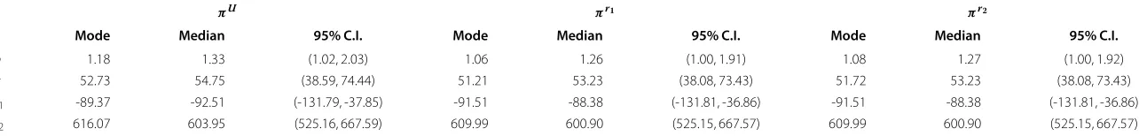
Table 1 presents the posterior summaries based on the priorsπU,πr1,πr2. For all three priors both the posterior mode and the posterior median forpare smaller than one. In addition, bothπr1- andπr2-based 95% credible intervals forpare contained in the interval (1, 2)indicating evidence that the errors are leptokurtic. In contrast, theπU-based 95% credible interval forpis not fully contained in the interval(1, 2). However, from the results in Section 4.1 we know that for small true values ofp, the use of theπUprior leads to on
average wider credible intervals forpthat have lower coverage than nominal. Thus, this application provides an example when the superiority of theπr1andπr2priors matters to the conclusion that in this data set the errors distribution is leptokurtic.
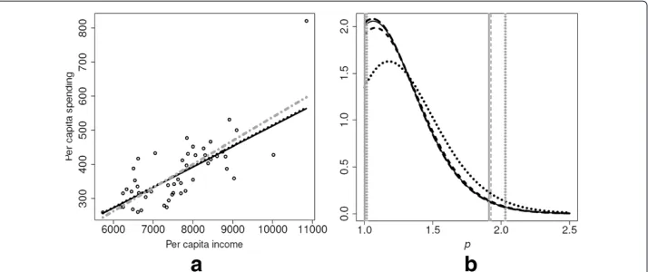
Figure 4(a) shows the scatterplot for the school spending data set along with the fit-ted EP regression model based on πr1 (solid line), πr2 (dashed line), and πU (dotted line). Figure 4(a) also shows the fitted Gaussian linear model (dot-dashed line). While the Gaussian model fit is clearly and strongly influenced by the outlier, the use of exponen-tial power errors (with the four priors considered here) automatically makes the analysis robust against outliers. In particular, the model fits using theπr1andπr2 priors (consid-ering the posterior median) coincide and are equal toy= −88.38+600.9x. Another way to make the analysis robust against outliers is to use t errors. Assuming Student-t errors, a model fiStudent-tStudent-ted by Fonseca eStudent-t al. (2008) wasy = −75.3+583.2x. We can see that both Student-t and exponential power errors fits are robust against outliers. How-ever, the Student-t distribution cannot accommodate platykurtic errors and, therefore, the exponential power distribution provides more flexibility.
Figure 4(b) presents the marginal posterior densities forpbased onπr1 (solid line), πr2 (dashed line),πr3 (long-dashed line) andπU (dotted line). In addition, the vertical lines indicate the limits of the 95% HPD credible intervals. The three reference priors lead to similar posterior densities forp, while theπU prior leads to a substantially dif-ferent posterior density forp. Figure 4(b) illustrates why theπU leads to unnecessarily
wider credible intervals. That combined withπU-based credible intervals having
cov-erage lower than nominal leads us to prefer the data analysis based on the reference priors.
4.2.2 Sold home videos vs. profits at the box office
Jo
urn
al
of
St
at
ist
ica
lD
is
tribut
io
n
s
an
d
A
pplica
tio
n
s2014,
1
:1
2
Page
11
o
f
20
a
jo
urna
l.co
m
/co
ntent/1/1/12
Table 1 School spending data set: Posterior summaries based on the noninformative priorπUand the reference priorsπr1andπr2
πU πr1 πr2
Mode Median 95% C.I. Mode Median 95% C.I. Mode Median 95% C.I.
p 1.18 1.33 (1.02, 2.03) 1.06 1.26 (1.00, 1.91) 1.08 1.27 (1.00, 1.92)
σ 52.73 54.75 (38.59, 74.44) 51.21 53.23 (38.08, 73.43) 51.72 53.23 (38.08, 73.43)
β1 -89.37 -92.51 (-131.79, -37.85) -91.51 -88.38 (-131.81, -36.86) -91.51 -88.38 (-131.81, -36.86)
Figure 4 School spending data set.(a)Scatterplot of the data and fitted EP regression model based onπr1
(solid line),πU(dotted line) and considering Gaussian linear model (dot-dashed line).(b)Marginal posterior densities forpbased onπr1(solid line),πr2(dashed line),πr3(long-dashed line) andπU(dotted line). Vertical
lines indicate the 95% HPD credible intervals, respectively.
Figure 5(a) shows the model fit for each of the priors we consider. The fits based on the reference priors visually coincide, whereas the fit based onπUis slightly different. This is
confirmed by Table 2, that shows that the slopes for the three fits are similar and around 4.33, whereas the intercept for theπU-based fit is about 4.5% larger than the intercept for theπr1- andπr2-based fits. Even more striking are the differences between the reference analyses and theπU-based analysis forσ andp. Forσ, both posterior medians based on πr1andπr2are very similar and equal to 67.37 and 68.38 respectively, while the posterior median based onπU is 77.50. Moreover, the 95% credible intervals forσ based onπr1 andπr2 are very similar and equal to(38.08, 93.64)and(38.10, 93.64)respectively, while the interval based onπUis substantially different and equal to(47.17, 98.69).
The reference analyses forpare also strikingly distinct from theπU-based analysis for
p. First, the posterior medians forpbased onπr1andπr2coincide and are equal to 2.64 while theπU-based posterior median differs tremendously and is equal to 4.36. Second, the 95% credible intervals forpbased onπr1andπr2are similar and equal to(1.00, 7.01) and(1.00, 7.18)respectively, while theπU-based interval forpdiffers tremendously from
Figure 5 Videos data set.(a)Scatterplot of the data and fitted EP regression model based onπr1(solid line),
πr2(dashed line),πr3(long-dashed line) andπU(dotted line).(b)Marginal posterior densities forpbased on
Jo
urn
al
of
St
at
ist
ica
lD
is
tribut
io
n
s
an
d
A
pplica
tio
n
s2014,
1
:1
2
Page
13
o
f
20
a
jo
urna
l.co
m
/co
ntent/1/1/12
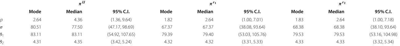
Table 2 Videos data set: Posterior summaries based on the noninformative priorπUand the reference priorsπr1andπr2
πU πr1 πr2
Mode Median 95% C.I. Mode Median 95% C.I. Mode Median 95% C.I.
p 2.64 4.36 (1.36, 9.64) 1.82 2.64 (1.00, 7.01) 1.83 2.64 (1.00, 7.18)
σ 80.51 77.50 (47.17, 98.69) 67.37 67.37 (38.08, 93.64) 68.38 68.38 (38.10, 93.64)
β1 83.11 83.11 (54.92, 107.65) 79.39 79.40 (53.03, 105.76) 79.53 79.53 (53.16, 104.98)
the reference CIs and is equal to(1.36, 9.64). Hence, theπU-based CI is more than 30% wider than the reference CIs. This undesirable feature ofπU-based CIs coincides with the results from the simulation study presented in Section 4.1.
Finally, Figure 5(b) presents the marginal posterior densities forpbased onπr1,πr2, andπU. This figure sheds light on the reason for the striking difference between theπr1 -andπr2-based CIs and theπU-based CI. The problem with theπU-based analysis is that the right tail of the marginal posterior density forpdecays too slowly. As a result, for the home video dataset theπU-based CI depends dramatically on the right side truncation of the prior, which in this manuscript has been fixed at 10. Figure 5(b) makes it really clear that a larger truncation point would have a huge impact in the resultingπU-based CI for
p. This dataset clearly illustrates the superiority of the Bayesian reference analyses.
5 Conclusions
We have developed Bayesian reference analysis for linear models with exponential power errors. Specifically, we have developed three reference priors that lead to useful proper posterior distributions. In addition, we have shown through a simulation study that both priors yield procedures that have better frequentist properties than procedures resulting from a competing noninformative prior. Finally, we have illustrated our Bayesian reference analysis methodology with two real world applications that highlight the flexibility of the exponential power distribution to accommodate both cases when there are outliers in the dataset and also cases when the errors follow a platykurtic distribution.
The fact that the reference priors we have obtained for the EP regression model lead to proper posterior distributions is of substantial theoretical interest. The propriety of these reference posterior distributions contrasts with the impropriety of the posterior distri-bution associated with the Jeffreys-rule prior found by Salazar et al. (2012). Moreover, Salazar et al. (2012) found two independence Jeffreys priors, one of which leads to an improper posterior distribution whereas the other leads to a proper posterior distribu-tion. We have found that the independence Jeffreys prior that yields a proper posterior distribution coincides with our reference priorπr1. Further, the independence Jeffreys prior that yields a useless improper posterior distribution differs only by a factor ofp−1/2
from the reference priorπr2. However, this difference is enough to make our reference priorπr2yield a useful proper posterior distribution.
Our results motivate many possible directions for future research. First, an open ques-tion is whether there exist general condiques-tions under which reference priors yield proper posterior distributions. In addition, the existence of general conditions for posterior pro-priety may be investigated for Jeffreys-rule and independence Jeffreys priors. The search of general conditions for posterior propriety may benefit from our present work on EP regression and previous literature on examples of impropriety of posterior distributions for distinct objective Bayes priors (Berger et al. 2001; Ferreira and De Oliveira 2007; Salazar et al. 2012; Wasserman 2000).
We have considered the frequentist properties of the proposed Bayesian approaches via a simulation study. In particular, we have shown that credible intervals based onπr1, πr2, andπr3 have similar frequentist properties with coverage close to nominal forpand σ. This is a reflection of the fact that for any prior satisfying some regularity conditions the frequentist coverage of credible intervals and the nominal level agree up toO(n−1/2)
stringent agreement of orderO(n−1) is called a first-order probability matching prior. Such priors have to be derived with a specific parameter of interest in mind, and their derivation is far from trivial. Therefore, promising directions for future research for the EP regression model would be the derivation of priors that lead to Bayesian predictions that have approximate frequentist validity (Datta et al. 2000b) and the derivation of first-order probability matching priors (Datta and Ghosh 1995; Datta et al. 2000a).
Appendix
Proof of Theorem 1.To prove Theorem 1, we follow the methodology to obtain refer-ence priors proposed by Berger and Bernardo (1992a). In particular, we assume that the reader is familiar with both the notation and the methodology of Berger and Bernardo (1992a). This proof is divided in two parts. In the first part, we obtain the reference prior for the orderings(β,σ,p),(σ,β,p), and(σ,p,β). Because the proofs are analogous for each of these three orderings, in the first part we obtain the reference prior for the order-ing(σ,β,p). In the second part, we obtain the reference prior for the orderings(β,p,σ), (p,β,σ), and(p,σ,β). Because the proofs are analogous for each of these three orderings, in the second part we obtain the reference prior for the ordering(p,β,σ).
Part 1.Consider the orderingθ =(σ,β,p).
After rearranging the Fisher information matrixH(θ)given in Equation (8) to conform to this ordering, the inverse of the Fisher information matrix becomes
S(θ)=H−1(θ)= ⎡ ⎢ ⎢ ⎣ σ2 np
(1+p−1) (1+p−1)
(1+p−1) (1+p−1)−1 0
σp
n (1+p−1) 1(1+p−1)−1
0 σ2p−12−p−1ni=1xixi −1
0 σp
n (1+p−1) 1(1+p−1)−1 0
p3
n (1+p−1) 1(1+p−1)−1
⎤ ⎥ ⎥ ⎦.
Thus,
S1= σ 2
np
1+p−1 1+p−1
1+p−1 1+p−1−1,
S2=
σ2 np
(1+p−1) (1+p−1)
(1+p−1) (1+p−1)−1 0
0 σ2p−12−p−1 n i=1xixi
−1
,
andS3=S(θ). Moreover, letHj=S−1j . Thus,
H1= np
σ2
1+p−1 1+p−1−1
1+p−1 1+p−1 ,
H2=
np
σ2
(1+p−1) (1+p−1)−1
(1+p−1) (1+p−1) 0
0 σ−2p−12−p−1 ni=1xixi
,
andH3=H(θ).
Lethjbe thenj×njlower right corner ofHj. Thus,
h1=
np
σ2
1+p−1 1+p−1−1
1+p−1 1+p−1 ,
h2=σ−2
p−12−p−1
n
i=1
xixi, and
h3=np−3
Let θ(1) = σ, θ(2) = β, and θ(3) = p. In addition, let θ[1] = θ(1) = σ, θ[2] = (θ(1),θ(2)) = (σ,β), and θ[3] = (θ(1),θ(2),θ(3)) = (σ,β,p). Moreover, let θ[∼1] = (θ(2),θ(3)) = (β,p) andθ[∼2] = (θ(3)) = p. Further, consider the following
compact sets: forσ,l(1)=[l−1,l]; forβ,l(2)=[−l,l]k; forp,l(3)=[1,l]. Then,
πl
3(p|σ,β)= π3l
θ[∼2]|θ[2]
= |h3(θ)| 1/21
l (3)
θ(3)
l
(3)|h3(θ)| 1/2dθ(
3)
=
np−31+p−1 1+p−11/21[1,l](p)
l 1
np−31+p−1 1+p−11/2dp = {c1(l)}−1p−3/2
1+p−11/2 1+p−11/21[1,l](p),
wherec1(l)=
l
1p−3/2(1+p−1)1/2
(1+p−1)1/2dp. Now,
πl
2(β,p|σ) = π2l
θ[∼1]|θ[1]
= π l 3
θ[∼2]|θ[2]
exp0.5El2log|h2(θ)|θ[2]
1l (2)
θ(2)
l (2)exp
0.5E2llog|h2(θ)|θ[2]
dθ(2)
,
where
El2log|h2(θ)|θ[2]
=
l (3)
log|h2(θ)|π3l(θ[∼2]|θ[2])dθ[∼2]
=
l
1
−2klogσ+klogp−1+klog2−p−1+log
n
i=1 xixi
{c1(l)}−1p−3/2
1+p−11/2 1+p−11/2dp = −2klogσ+c2(l),
with
c2(l) = {c1(l)}−1
l
1
klogp−1+klog2−p−1+log
n
i=1 xixi
p−3/21+p−11/2 1+p−11/2dp.
Hence,
πl
2(β,p|σ) = πl
3(p|σ,β)exp
0.5[−2klogσ+c2(l)]
1[−l,l]k(β)
[−l,l]kexp
0.5[−2klogσ+c2(l)]
dβ
= πl
3(p|σ,β)(2l)−k1[−l,l]k(β).
Finally,
πl
1(σ,β,p) = π1l
θ[∼0]|θ[0]
= π l 2
θ[∼1]|θ[1]
exp0.5El1log|h1(θ)|θ[1]
1l (1)
θ(1)
l (1)exp
0.5El1log|h1(θ)|θ[1]
dθ(1)
with
El1log|h1(θ)|θ[1]
= [−l,l]k l 1 log np σ2
1+p−1 1+p−1−1
1+p−1 1+p−1
πl
2(β,p|σ)dpdβ
= −2 logσ+c3(l),
where
c3(l)=
[−l,l]k l 1 log np
1+p−1 1+p−1−1
1+p−1 1+p−1
πl
2(β,p|σ)dpdβ
does not depend onθ =(σ,β,p). Hence,
πl
1(σ,β,p) = πl
2(β,p|σ)exp{0.5[2 logσ+c3(l)]}1(l−1,l)(σ)
l
l−1exp{0.5[2 logσ+c3(l)]}dσ
= π2l(β,p|σ)σ−11(l−1,l)(σ) 2 logl
Thus,
πl
1(σ,β,p)=σ−1p−3/2
1+p−11/2 1+p−11/2
× {c1(l)}−1(2l)−k(2 logl)−11[l−1,l](σ )1[−l,l]k(β)1[1,l](p).
Now take any pointθ∗ = (σ∗,β∗,p∗) ∈[l−1,l]×[−l,l]k×[1,l]. Then, the reference
prior for the ordering(σ,β,p)is
π(σ,β,p) ∝ lim
l→∞ πl
1(σ,β,p) πl
1(σ∗,β∗,p∗)
= σ−1p−3/21+p−11/2 1+p−11/2,
which is of the form (4).
Part 2.Consider the orderingθ =(p,β,σ).
After rearranging the Fisher information matrixH(θ)given in Equation (8) to conform to this ordering, the inverse of the Fisher information matrix becomes
S(θ)=H−1(θ)= ⎡ ⎢ ⎢ ⎣ p3 n 1
(1+p−1) (1+p−1)−1 0 σpn (1+p−1) 1(1+p−1)−1 0 σ2p−12−p−1 ni=1xixi
−1
0 σp
n (1+p−1) 1(1+p−1)−1 0 σ
2
np (1+
p−1) (1+p−1)
(1+p−1) (1+p−1)−1 ⎤ ⎥ ⎥ ⎦,
Thus,
S1= p3
n
1
1+p−1 1+p−1−1,
S2=
p3
n (1+p−1) 1(1+p−1)−1 0
0 σ2(p−1)2−p−1 ni=1xixi
−1
,
andS3=S(θ). Moreover, letHj=S−1j . Thus,
H1=np−3{(1+p−1) (1+p−1)−1},
H2=
np−3{1+p−1 1+p−1−1} 0
0 σ−2p−12−p−1 ni=1xixi
,
Lethjbe thenj×njlower right corner ofHj. Thus,
h1=np−3{(1+p−1) (1+p−1)−1},h2=σ−2p−12−p−1
n
i=1
xixi, andh3=npσ−2.
Letθ(1)=p,θ(2)=β, andθ(3) =σ. In addition, letθ[1] =θ(1)=p,θ[2]=(θ(1),θ(2))= (p,β), andθ[3]=(θ(1),θ(2),θ(3))=(p,β,σ). Moreover, letθ[∼1]=(θ(2),θ(3))=(β,σ)and θ[∼2] =(θ(3))=σ. Further, consider the following compact sets: forp,l(1) =[1,l]; for β,l(2)=[−l,l]k; forσ,l(3)=[l−1,l].
Then,
πl
3(σ |p,β)= π3l
θ[∼2]|θ[2]
= |h3(θ)| 1/21
l (3)
θ(3)
l
(3)|h3(θ)| 1/2dθ(
3)
=
npσ−21/21[l−1,l](σ)
l
l−1
npσ−21/2dσ = σ−1(2 logl)−11[l−1,l](σ).
Moreover,
πl
2(β,p|σ) = π2l(θ[∼1]|θ[1])
= π l
3(θ[∼2]|θ[2])exp
0.5El2log|h2(θ)|θ[2]
1l (2)(θ(2))
l (2)exp
0.5E2llog|h2(θ)|θ[2]
dθ(2)
,
where
E2llog|h2(θ)|θ[2]
=
l (3)
log|h2(θ)|π3l(θ[∼2]|θ[2])dθ[∼2]
=
l
l−1
−2klogσ+klog(p−1)+klog(2−p−1)+log
n
i=1 xixi
σ−1(2 logl)−1dσ
= c1(l,p), which does not depend onβ.
Hence,
πl
2(β,σ |p) = πl
3(σ|p,β)exp
0.5c1(l,p)
1[−l,l]k(β)
[−l,l]kexp
0.5c1(l,p)
dβ = πl
3(σ|p,β)(2l)−k1[−l,l]k(β).
Further,
πl
1(p,β,σ)= π1l(θ[∼0]|θ[0])
= π l
2(θ[∼1]|θ[1])exp
0.5El1log|h1(θ)|θ[1]
1l (1)(θ(1))
l (1)exp
0.5El1log|h1(θ)|θ[1]
dθ(1)
,
with
E1llog|h1(θ)|θ[1]
=
[−l,l]k
l
l−1log
np−3{(1+p−1) (1+p−1)−1}π2l(β,σ |p)dσdβ
Hence,
πl
1(σ,β,p) = πl
2(β,σ|p)exp{0.5 log
np−3{(1+p−1) (1+p−1)−1}}1(1,l)(p)
l
1exp{0.5 log
np−3{(1+p−1) (1+p−1)−1}}dp = πl
2(β,p|σ)p−3/2{(1+p−1) (1+p−1)−1}1/2c2(l)1[1,l](p),
where
{c2(l)}−1=
l
1
exp{0.5 lognp−3{(1+p−1) (1+p−1)−1}}dp.
Thus,
πl
1(p,β,σ )=σ−1p−3/2{(1+p−1) (1+p−1)−1}1/2c2(l)(2l)−k(2 logl)−11[1,l](p)1[−l,l]k(β)1[l−1,l](σ ).
Now take any pointθ∗ = (p∗,β∗,σ∗) ∈ [1,l]× [−l,l]k× [l−1,l]. Then, the reference prior for the ordering(p,β,σ)is
π(p,β,σ) ∝ lim
l→∞ πl
1(p,β,σ) πl
1(p∗,β∗,σ∗)
= σ−1p−3/2{(1+p−1) (1+p−1)−1}1/2,
which is of the form (4).
Competing interests
The authors declare that they have no competing interests.
Authors’ contributions
MARF proved Theorem 1, Lemma1, and Proposition 1, and wrote the manuscript. ES performed the computations for the simulation study and for the application, and wrote the manuscript. Both authors read and approved the final manuscript.
Acknowledgement
The work of Ferreira was supported in part by National Science Foundation Grant DMS-0907064. The authors gratefully acknowledge the constructive comments and suggestions made by three anonymous referees that led to a substantially improved article.
Author details
1Department of Statistics, University of Missouri, Columbia, USA.2Department of Electrical and Computer Engineering,
Duke University, Durham, USA.
Received: 17 October 2013 Accepted: 11 April 2014 Published: 17 June 2014
References
Achcar, JA, Pereira, GA: Use of exponential power distributions for mixture models in the presence of covariates. J. Appl. Stat.26(6), 669–679 (1999)
Berger, JO, Bernardo, JM: On the development of the reference prior method. In: Bernardo, JM, Berger, JO, Dawid, AP, Smith, AFM (eds.) Bayesian Statistics 4, pp. 35–60. Oxford University Press, London, (1992a)
Berger, JO, Bernardo, JM: Ordered group reference priors with applications to a multinomial problem. Biometrika
79, 25–37 (1992b)
Berger, JO, Bernardo, JM: Reference priors in a variance components problem. In: Goel, PK, Iyengar, NS (eds.)Bayesian Analysis in Statistics and Econometrics, pp. 323–340. Springer, Berlin, (1992c)
Berger, JO, de Oliveira, V, Sansó, B: Objective Bayesian analysis of spatially correlated data. J. Am. Stat. Assoc.96(456), 1361–1374 (2001)
Bernardo, JM: Reference posterior distribution for Bayes inference. J. Roy. Stat. Soc. B.41, 113–147 (1979) Bernardo, JM, Smith, AFM: Bayesian Theory. Wiley, New York (1994)
Box, GEP, Tiao, GC: A further look at robustness via Bayes’s theorem. Biometrika.49, 419–432 (1962) Box, GEP, Tiao, GC: Bayesian Inference in Statistical Analysis. Wiley-Interscience, Hoboken (1992)
Choy, STB, Smith, AFM: On robust analysis of a normal location parameter. J. Roy. Stat. Soc. B.59(2), 463–474 (1997) Cribari-Neto, F, Ferrari, SLP, Cordeiro, GM: Improved heteroscedasticity-consistent covariance matrix estimators.
Biometrika.87, 907–918 (2000)
Datta, GS, Ghosh, JK: Noninformative priors for maximal invariant parameter in group models. Test.4, 95–114 (1995) Datta, GS, Ghosh, M, Mukerjee, R: Some new results on probability matching priors. Bull. Calcutta Stat. Assoc.
50(199–200), 179–192 (2000a)
Datta, GS, Mukerjee, R, Ghosh, M, Sweeting, TJ: Bayesian prediction with approximate frequentist validity. Ann. Stat.
Ferreira, MAR, De Oliveira, V: Bayesian reference analysis for Gaussian Markov Random Fields. J. Multivariate Anal.98, 789–812 (2007)
Ferreira, MAR, Suchard, MA: Bayesian analysis of elapsed times in continuous-time Markov chains. Can. J. Stat.36, 355–368 (2008)
Fonseca, TCO, Ferreira, MAR, Migon, HS: Objective Bayesian analysis for the Student-tregression model. Biometrika.
95(2), 325–333 (2008)
Greene, WH: Econometric Analysis. Prentice-Hall, Upper Saddle River (1997)
Ghosh, JK, Delampady, M, Samanta, T: An Introduction to Bayesian Statistics – Theory and Methods. Springer, New York (2006)
Jeffreys, H: Theory of Probability. Oxford University Press, Oxford (1961)
Levine, DM, Krehbiel, TC, Berenson, ML: Business Statistics: A First Course. Pearson Prentice Hall, Upper Saddle River (2006) Liang, F, Liu, C, Wang, N: A robust sequential Bayesian method for identification of differentially expressed genes.
Statistica Sinica.17, 571–597 (2007)
Salazar, E, Ferreira, MAR, Migon, HS: Objective Bayesian analysis for exponential power regression models. Sankhya -Series B.74, 107–125 (2012)
Sun, D, Berger, JO: Objective Bayesian analysis for the multivariate normal model. In: Bernardo, JM, Bayarri, MJ, Berger, JO, Dawid, AP, Heckerman, D, Smith, AFM, West, M (eds.) Bayesian Statistics 8, pp. 525–547. Oxford University Press, Oxford, (2007)
Vianelli, S: La misura della variabilità condizionata in uno schema generale delle curve normali di frequenza. Statistica.23, 447–474 (1963)
Walker, SG, Gutiérrez-Peña, E: Robustifying Bayesian procedures. In: Bayesian Statistics 6. Oxford University Press, New York, (1999)
Wasserman, L: Asymptotic inference for mixture models using data-dependent priors. J. Roy. Stat. Soc. B.62, 159–180 (2000)
West, M: Outlier models and prior distributions in Bayesian linear regression. J. Roy. Stat. Soc. B.46, 431–439 (1984) West, M: On scale mixtures of normal distributions. Biometrika.79, 646–648 (1987)
Zhu, D, Zinde-Walsh, V: Properties and estimation of asymmetric exponential power distribution. J. Econometrics.148, 86–99 (2009)
doi:10.1186/2195-5832-1-12
Cite this article as:Ferreira and Salazar:Bayesian reference analysis for exponential power regression models.Journal of Statistical Distributions and Applications20141:12.
Submit your manuscript to a
journal and benefi t from:
7Convenient online submission 7Rigorous peer review
7Immediate publication on acceptance 7Open access: articles freely available online 7High visibility within the fi eld
7Retaining the copyright to your article