and Quantitative Risk DOI 10.1186/s41546-019-0036-4
R E S E A R C H Open Access
Piecewise constant martingales and lazy clocks
Christophe Profeta· Fr´ed´eric Vrins
Received: 1 March 2018 / Accepted: 17 January 2019 /
© The Author(s). 2019Open AccessThis article is distributed under the terms of the Creative Commons Attribution 4.0 International License (http://creativecommons.org/licenses/by/4.0/), which permits unrestricted use, distribution, and reproduction in any medium, provided you give appropriate credit to the original author(s) and the source, provide a link to the Creative Commons license, and indicate if changes were made.
Abstract Conditional expectations (like, e.g., discounted prices in financial applica-tions) are martingales under an appropriate filtration and probability measure. When the information flow arrives in a punctual way, a reasonable assumption is to sup-pose the latter to have piecewise constant sample paths between the random times of information updates. Providing a way to find and constructpiecewise constant mar-tingalesevolving in a connected subset ofRis the purpose of this paper. After a brief review of possible standard techniques, we propose a construction scheme based on the sampling of latent martingalesZ˜ withlazy clocksθ. Theseθare time-change pro-cesses staying in arrears of the true time but that can synchronize at random times to the real (calendar) clock. This specific choice makes the resulting time-changed pro-cessZt = ˜Zθta martingale (called alazy martingale) without any assumption onZ˜, and in most cases, the lazy clockθis adapted to the filtration of the lazy martingale Z, so that sample paths of Z on[0, T]only requires sample paths ofθ,Z˜up toT. This would not be the case if the stochastic clockθcould be ahead of the real clock, as is typically the case using standard time-change processes. The proposed approach yields an easy way to construct analytically tractable lazy martingales evolving on (interval of)R.
Keywords Time-change process·Last passage time·Martingale·Bounded martingale·Jump martingale·Subordinator
Christophe Profeta Universit´e d’ ´Evry, France Fr´ed´eric Vrins ()
Louvain Finance Center (LFIN) and Center for Operations Research and Econometrics (CORE), Voie du Roman Pays 34, 1348 Louvain-la-Neuve, Belgium
1 Introduction
Martingales play a central role in probability theory, but also in many applications. This is specifically true in mathematical finance where it is used to model Radon— Nikodym derivative processes or discounted prices in arbitrage-free market models (Jeanblanc et al.2007). More generally, it is very common to deal with conditional expectation processesZ=(Zt)t∈[0,T], Zt :=E[ZT|Ft], whereF:=(Ft)t∈[0,T]is a
reference filtration andEstands for the expectation operator associated with a given probability measureP. Many different modeling setups have been proposed to repre-sent the dynamics ofZ(e.g., random walk, Brownian motion, Geometric Brownian motion, Jump diffusion, etc) depending on some assumptions about its range, path-wise continuity, or continuous versus discrete-time setting. In many circumstances, however, information can be considered to arrive at random times, or in a partial (punctual way).
An interesting application in that respect is the modeling ofquoted recoveryrates. The recovery raterof a firm corresponds to the ratio of the debt that will be recovered after the firm’s default during an auction process. It is also a major factor driving the price of corporate bonds or other derivatives instruments likes credit default swaps or credit linked notes. In many standard models (like those suggested by the Inter-national Swaps and Derivatives Association (ISDA)), the recovery rate process is assumed constant (see e.g., Markit (2004)). Many studies stressed the fact that ris in fact not a constant: it cannot be observed prior to the firm’s defaultτ; r is an Fτ-measurable random variable in[0,1]. This simple observation can have serious
consequences in terms of pricing and risk-management of credit sensitive products, and explains the development of stochastic recovery models (Amraoui et al.2012, Andersen and Sidenius2004). A further development in credit risk modeling is to take into account the fact that recovery rates can be “dynamized” (Gaspar and Slinko 2008). Quoted recovery rates, for instance, can thus be modeled as a stochastic pro-cessR = (Rt)t≥0that gives the “market’s view” of a firm’s recovery rate as seen from timet. Hence,Rt :=E[r|Ft]can be seen as a martingale evolving in the unit
interval. By correlatingRwith the creditworthiness of the firm, it becomes possible to account for a well-known fact in finance: recovery rate and default probability are statistically linked (Altman et al.2003). However, observations for the processRare limited: updates in recovery rate quotes arrive in a scarce and random way. Therefore, in contrast with the common setup, it is more realistic to representR as a martin-gale whose trajectories remain constant for long period of times, but “changes” only occasionally, upon arrival of related information (e.g., when a dealer updates its view to specialized data providers). More generally, such types of martingales could be used to model discounted price processes of financial instruments, observed under partial (punctual) information, e.g., at some random times, but also to represent price processes of illiquid products. Indeed, without additional information, a reasonable approach may consist of assuming that discounted prices remain constant between arrivals of market quotes, and jump to the level given by the new quote when a new trade is done.
piecewise constant sample paths. In this paper, we propose a methodology to find and construct such types of martingales. The special case ofstep-martingales(which are martingales with piecewise constant sample paths, but restricted to a finite num-ber of jumps in any finite interval) have been studied in Boel et al. (1975a,b), with emphasis on representation theorems and applications to communication and control problems. In Herdegen and Herrmann (2016), the authors investigate a single jump case, in which the first part of the path (before the unique jump) is supposed to be deterministic. We extend this research in several ways. First, we relax the (strong) step-martingale restriction and deal with the broader class of processes featuring pos-sibly infinitely many jumps in a time interval. Second, our approach allows one to build martingales that evolve in a bounded interval, a problem that received little attention so far and which relevance is stressed with the above recovery example, but could also be of interest for modeling stochastic probabilities or correlations. This is achieved by introducing a new class of time-change processes calledlazy clocks. Finally, we provide and study numerous examples and propose some construction algorithms.
The paper is organized as follows. In Section2we formally introduce the con-cept ofpiecewise constant martingales Z and presents several routes to construct these processes. We then introduce a different approach in Section3, where(Zt)t≥0 is modeled as a time-changed processZ˜θt
t≥0, whereθ is alazy clock. The latter are time-change processes built in such a way that the stochastic clock always stays in arrears of the real clock (θt ≤ t a.s.). This condition is motivated by
computa-tional considerations: it guarantees that samplingZover a fixed time horizon[0, T] only requires the sampling of
˜ Z, θ
over the same period. Finally, as our objective is to provide a workable methodology, we derive the analytical expression for the distributions and moments in some particular cases, and provide efficient sampling algorithms for the simulations of such martingales.
2 Piecewise constant martingales
In the literature, pure jump processes defined on a filtered probability space (,F,F,P), whereF=(Ft)t∈[0,T]andF :=FT, are often referred to as
stochas-tic processes having no diffusion part. In this paper we are interested in a subclass of pure jump processes:piecewise constant (PWC) martingalesdefined as follows.
Definition 1(Piecewise constant martingale)A piecewise constantF-martingale Z is a c`adl`ag F-martingale whose jumps Zs = Zs −Zs− are summable (i.e.
s≤T|Zs|<+∞a.s.) and such that for everyt ≥0:
Zt =Z0+
s≤t Zs .
Note that an immediate consequence of this definition is that a PWC martingale has finite variation. Such type of processes may be used to represent martingales observed under partial (punctual) information, e.g. at some (random) times. One pos-sible field of application is mathematical finance, where discounted price processes are martingales under an equivalent measure. Without additional information, a rea-sonable approach may consist in assuming that discounted prices remain constant between arrivals of market quotes, and jump to the level given by the new quote when a new trade is done. More generally, this could represent conditional expectation processes (i.e. “best guess”) where information arrives in a discontinuous way.
Most of the “usual” martingales with no diffusion term fail to have piece-wise constant sample paths. For example, Az´ema’s first martingaleM = (Mt)t≥0 defined as
Mt :=sign(Wt)
π 2
t−gt0(W ) , g0t(W ):=sup{s≤t, Ws =0}, (1)
whereW is a Brownian motion, is essentially piecewise square-root. Interestingly, one can show thatMt =E
Wt|Fg0
t(W )+ , so thatMactually corresponds to the pro-jection ofW onto itsslow filtration, see e.g. Dellacherie et al. (1992) and Mansuy and Yor (2006) and Chapter IV, section 8 of Protter (2005) for a detailed analysis of this process. Similarly, the Geometric Poisson Process eNtlog(1+σ )−λσ t is a posi-tive martingale with piecewise negaposi-tive exponential sample paths (Shreve2004, Ex 11.5.2).
However, finding such type of processes is not difficult. We provide below three different methods to construct some of them. Yet, not all are equally powerful in terms of tractability. The last method proves to be quite appealing in that it yields analytically tractable PWC martingales whose range can be any connected set.
2.1 An autoregressive construction scheme
We start by looking at a subset of PWC martingales, namely step-martingales. These are martingales whose paths belong to the space of step functions on any bounded interval, i.e. whose paths are a finite linear combination of indicator functions of intervals. As a consequence, a step martingaleZadmits a finite number of jumps on
[0, T]taking places at, say(τk, k≥1), and may be decomposed as (withτ0=0)
Zt =Z0+
+∞
k=1
Zτk −Zτk−1
1{τk≤t}.
Looking at such decomposition, we see that step martingales may easily be constructed by an autoregressive scheme.
Proposition 1Let Z be a c`adl`ag process with integrable variation starting from Z0. We assume thatE[|Z0|]<+∞. Then, the following are equivalent:
ii) there exists a strictly increasing sequence of random times(τk, k≥ 0)starting
fromτ0 =0, taking values in[0,+∞]and with no point of accumulation such that
Zt :=Z0+
+∞
k=1
Zτk −Zτk−1
1{τk≤t} (2)
and which satisfies for any0≤s≤t:
+∞
k=1
EZτk−Zτk−1
1{s<τk≤t}Fs
=0. (3)
Furthermore, the filtration F is given for s ≥ 0 by Fs = σ
Zτk, τk
for k≥0such thatτk ≤s).
Proof i)−→ii) LetZbe a step-martingale with respect to its natural filtrationF, and denote by(τk, k ≥ 0)the sequence of its successive jumps, withτ0 = 0. IfZ only admits a finite number of jumpsn0, then we setτn = +∞forn > n0. This choice of the sequence(τk, k≥0)implies that the filtrationFequals
Fs =σ (Zu, u≤s)=σZτk, τk
forτk ≤s, s≥0
and that we have the representation :
Zt =Z0+
+∞
k=1
Zτk −Zτk−1
1{τk≤t}.
Taking the expectation with respect toFs with 0 ≤ s ≤ t on both sides and
applying Fubini’s theorem (sinceZis of integrable variation), we deduce that :
Zs =Z0+
+∞
k=1
EZτk −Zτk−1
1{τk≤t}|Fs
=Z0+
+∞
k=1
Zτk−Zτk−1
1{τk≤s}+ +∞
k=1
EZτk−Zτk−1
1{s<τk≤t}|Fs
which implies that the second sum on the right-hand side is null. ii)−→i) Define
Zt =Z0+
+∞
k=1
Zτk−Zτk−1
1{τk≤t},
and observe that since the sequence(τk, k ≥ 0)has no point of accumulation,Z is
clearly a step process. Furthermore, sinceZis of integrable variation, we have
E[|Zt|] ≤E[|Z0|]+E
+∞
k=1
Zτk−Zτk−1
1{τk≤t}
≤E[|Z0|]+E ⎡
⎣
0<s≤t
|Zs−Zs−|
which prove thatZtis integrable for anyt≥0. Finally, as in the first part of the proof, taking
the expectation with respect toFsin (2) and using (3), we deduce that :
E[Zt|Fs] =Z0+
+∞
k=1
Zτk−Zτk−1
1{τk≤s}+
+∞
k=1
EZτk−Zτk−1
1{s<τk≤t}|Fs
=Zs
which proves thatZis indeed a martingale.
Corollary 1Let M be a martingale of integrable variation, and let(τk, k ≥ 0)
be an increasing sequence of random times starting fromτ0 = 0, taking values in (0,+∞], with no point of accumulation and which is independent of M. Then, ifZ0 is an integrable random variable, the process
Zt =Z0+
+∞
k=1
Mτk−Mτk−1
1{τk≤t}, t≥0
is a step martingale with respect to the filtrationF given, for s ≥ 0, by Fs = σMτk, τk
fork≥1such thatτk≤s
.
ProofWe only need to check that (3) is satisfied, which is a consequence of the tower property of conditional expectations. Indeed, define the larger filtrationGs = σ ((τi, i≥1), (Mu, u≤s))and observe that on the set{s < τk ≤t}:
Fs ⊂Fτk−1⊂Gτk−1.
Then, sinceMis aG-martingale :
EMτk−Mτk−1
1{s<τk≤t}|Fs
=EE Mτk−Mτk−1Gτk−1
1{s<τk≤t}|Fs
=EE Mτk−1−Mτk−1Gτk−1
1{s≤τk−1<τk≤t}|Fs
=0.
Remark 1Observe that the natural filtration of Z in Proposition1satisfies the identityFt =Fτk on the set{τk ≤t < τk+1}. Since the random times(τk, k≥0)are stopping times in the filtrationF, this implies thatFis a jumping filtration, following the definition of Jacod-Skorokhod (1994).
Example 1Let N be a counting process and letτ1, . . . , τNt be the sequence of jump times of N on[0, t]withτ0:=0. If(Yk, k ≥1)is a family of independent and
centered random variables, independent from N, then
Zt :=Z0+
∞
k=1
Yk1{τk≤t}=Z0+ Nt
k=1
Yk, Z0∈R
is a PWC martingale. Note that we may choose the range of such a PWC martingale by taking bounded random variables. For instance, ifZ0=0and for anyk≥1,
P
6a
π2k2 ≤Yk≤ 6b π2k2
=1
The above corollary provides us with a simple method to construct PWC mar-tingales. Yet, it suffers from two restrictions. First, the distribution ofZt requires
averaging the conditional distribution with respect to the counting process, which may be an infinite sum. Second, a control on the range of the resulting martin-gale requires strong assumptions. One might try to relax the i.i.d. assumption of the Yk’s. In Example 1the Yk’s are independent but their support decreases as 1/k2.
One could also drawYk from a distribution whose support is state dependent like
a−Zτk−1, b−Zτk−1
, thenZt ∈ [a, b]for allt ∈ [0, T]. In the sequel, we address
these drawbacks by proposing another construction scheme.
2.2 PWC martingales from pure jump martingales with vanishing compensator
Pure jump martingales can easily be obtained by taking the difference of a pure jump increasing process with a predictable, grounded, right-continuous process of bounded variation (calleddual predictable projectionsorpredictable compensator). The sim-plest example is probably the compensated Poisson process of parameterλdefined by(Mt =Nt −λt, t ≥ 0). This process is a pure jump martingale with piecewise
linearsample paths, hence is not a PWC martingale as s≤tMs = Nt = Mt.
However, it is easy to see that the difference of two Poisson processes with the same intensity is a PWC martingale (in fact a step-martingale), and we shall generalize this idea in the following proposition.
Proposition 2AF-martingale of integrable variation Z (withZ0=0) is PWC if and only if there exist twoF-adapted, integrable and increasing pure jump processes A and B having the same dual predictable projections (i.eAp = Bp) such that Z=A−B.
ProofAssume first thatZis a PWC martingale of integrable variation. We define
At =
1 2
s≤t
(|Zs| +Zs) and Bt =
1 2
s≤t
(|Zs| −Zs) .
ThenA andBare two increasing pure jump processes such that Z = A−B. They are integrable since Z is of integrable variation, and they satisfy Ap−Bp=(A−B)p=Zp =0 which proves the first implication.
Assume now thatAandBare pure jump increasing processes. We then have the representation
Zt =At−Bt =
s≤t As−
s≤t Bs =
s≤t
(As −Bs)=
s≤t Zs .
By the triangular inequality, we may check that
|Zt| ≤
s≤t
|Zs| ≤
s≤t
|As| +
s≤t
henceZ is integrable and of integrable variation. Finally, by definition of the pre-dictable dual projections, the processesA−ApandB−Bpare martingales, hence by difference, so isZsinceAp=Bp.
An easy application of this result is the case of L´evy processes, for which the compensators are deterministic functions.
Corollary 2LetA, Bbe two L´evy processes having the same L´evy measureν, and consider a measurable function f such thatf (0) =0andR|f (x)|ν(dx) < +∞. Then the process
Zt =
s≤t
f (As)−f (Bs)
is a PWC martingale.
ProofThe proof follows from the fact that the compensator of
s≤tf (As), t ≥0is the deterministic processtRf (x)ν(dx), t ≥0.
Remark 2A centered L´evy process Z is a PWC martingale if and only if it has no drift, no Brownian component and its L´evy measureν satisfies the integrability conditionR|x|ν(dx) <∞.
As obvious examples, one can mention the difference of two independent Gamma or Poisson processes of same parameters. Note that stable subordinators are not allowed here, as they do not fulfill the integrability condition required onAandB. We give below the PDF of these two examples :
Example 2LetN1, N2be two independent Poisson processes with parameterλ. Then,Z :=N1−N2is a step martingale taking integer values, with marginal laws given by the Skellam distribution with parametersμ1=μ2=λt :
fZt(k)=e− 2λt
I|k|(2λt), k∈Z, (4)
whereIkis the modified Bessel function of the first kind.
Example 3Let γ1, γ2 be two independent Gamma processes with parameters a, b >0. Then,Z:=γ1−γ2is a PWC martingale with marginals given by
fZt(z)= b √
π (at)
bz2at−
1 2
K12−at(b|z|) , (5)
whereKβ denotes the modified Bessel function of the second kind with parameter β∈R.
ProofThe PDF ofZt is given, for 2at >1, by the inverse Fourier transform, see
Gradshteyn and Ryzhik (2007, p. 349 Formula 3.385(9)) :
fZt(z)= 1 2π
R
e−iuz
The result then follows by analytic continuation.
We conclude this section with an example of PWC martingale which does not belong to the family of L´evy processes but has the interesting feature to evolve in a time-dependent range.
Corollary 3LetR1, R2be two squared Bessel processes of dimensionδ ∈(0,2). Fori=1,2set
gt0
Ri
:=sup
s≤t, Rsi=0
.
Then,Z :=g0R1−g0R2is a 1-self-similar PWC martingale which evolves in the cone{[−t, t], t≥0}.
ProofLetRbe a squared Bessel processes of dimensionδ ∈(0,2)and denote by L0(R)its local time at 0 as given by Tanaka’s formula. Set
Yt =
t−gt0(R)
1−δ2
, t ≥0.
In Rainer (1996, Prop. 4.1 and 6.2.1), it is proven that the process X = Y − 1
22−δ22−δ2
L0(R)is a martingale with respect to the slow filtrationFg0 t+, t ≥0
.
We shall prove that
2 2−δg
0
t(R)−t, t≥0
is also a martingale in the same filtration. Notice first that since the random variable gt0(R)follows the generalized Arcsine law (see Section3.1.2below), the expectation of this process is constant and equal 0. We then apply Itˆo’s formula toY with the functionf (y)=y2−2δ :
t−gt0(R)=
t
0 2 2−δY
δ 2−δ s− dYs+
s≤t Y
2 2−δ
s −Y
2 2−δ
s− −
2 2−δ
s−g0s−(R) δ 2
Ys .
Observe next that the instants of jumps ofY are the same as those ofg0(R), i.e.
{s;Ys =Ys−} =
s;gs0(R)=g0s−(R)
. But, the jumps of g0(R) only happen at timesswhenRs =0, in which casegs0(R)=sor equivalentlyYs =0. This yields
the simplifications :
t−gt0(R)=
2 2−δ
t
0 Y
δ 2−δ s− dYs+
s≤t
−s−g0s−(R)
+2−2δs−gs0−(R)
δ 2
s−g0s−(R)
1−δ 2
= 2−2δ t 0
Y
δ 2−δ s− dYs+
2
2−δ−1
s≤t
g0s(R)−g0s−(R)
= 2
2−δ t
0 Y
δ 2−δ s− dYs+
2 2−δ−1
gt0(R)
and it remains to prove that the stochastic integral is a martingale. Since the support ofdL0(R)is included in{s; Rs = 0} ⊂ {s;Ys =0}, andL0(R)is continuous, we
t
0 Y
δ 2−δ
s− dL0s(R)=
t
0 Y
δ 2−δ
s dL0s(R)=0
hence the process
t− 2 2−δg
0
t(R)=
t
0 Y
δ 2−δ
s− dYs =
t
0 Y
δ 2−δ s− dXs
is a local martingale. To prove that it is a true martingale, choose an horizonT and observe that the process
t− 2 2−δg
0
t(R)+
2
2−δT ,0≤t ≤T
is now a positive local martingale, hence a supermartingale with constant expectation, hence a true martingale. Finally, the self-similarity ofg0t(R)comes from that ofR (see Revuz—Yor1999, Proposition 1.6, p. 443). Indeed, for any fixedt >0 :
g0t(R)=sup{s≤t, Rs=0} (law)
= sup{s≤t, tRs/t=0} =tsup{u≤1, Ru=0} =t g01(R) .
Remark 3When δ = 1, we haveX = W2 where W is a standard Brownian motion. Using L´evy Arcsine law, the PDF ofZ1is given by the convolution, forz∈ [0,1]:
fZ1(z)=
1 π2
1−z
0
1
√
x(1−x)
1
√
(z+x)(1−z−x)dx = 2 π2F
π 2,
1−z2 ,
where F denotes the incomplete elliptic integral of the first kind, see Gradshteyn and Ryzhik (2007, p. 275, Formula 3.147(5)). This yields, by symmetry and scaling :
fZt(z)= 2 π2
π 2
0
dx
t2cos2(x)+z2sin2 (x)
1{0<|z|≤t}.
Both the recursive and the vanishing compensators approaches are rather restric-tive in terms of attainable range and analytical tractability. In the next subsection, we provide a more general method that can be used to build PWC martingales to any connected set ofRin a simple and tractable way.
2.3 PWC martingales using time-changed techniques
In this section, we construct a PWC martingaleZby time-changing a latent (P,F )-martingaleZ˜ =
˜ Zt
t≥0with the help of a suitabletime-change processθ.
Definition 2(time change process) AF-time change processθ = (θt)∈[0,T]is a
stochastic process satisfying
• θ0=0,
Under mild conditions stated below,Z :=Z˜θt
t≥0is proven to be a martingale with respect to its own filtration, with the desired piecewise constant behavior. Most results regarding changed martingales deal with continuous martingales time-changed with a continuous process (Cont and Tankov2004, Jeanblanc et al.2007, Revuz and Yor1999). This does not provide a satisfactory solution to our problem as the resulting martingale will obviously have continuous sample paths. On the other hand, it is obvious that not all time-changed martingales remain martingales, so that conditions are required onZ˜ and/or onθ.
Remark 4EveryF-martingale time-changed with aF-adapted process remains a semi-martingale but not necessarily a martingale. For instance, settingZ˜ = W andθt =inf{s : Ws > t}thenZ˜θt = t. Also, ifθis independent fromZ˜, then the martingale property is always satisfied, but Z may fail to be integrable. For example ifZ˜ = W andθ is an independentα-stable subordinator withα = 1/2then the time-changed process Z is not integrable:EZ˜θt
|θt =
2
π √
θt andE
√ θt
is undefined. The proposition below gives sufficient conditions for Z to be integrable.
Proposition 3LetZ˜ be a martingale, andθbe a time-change process independent fromZ˜. We assume thatθhas PWC paths and that one of the following assumptions hold :
1. Z˜ is a positive martingale, 2. Z˜ is uniformly integrable,
3. there exists an increasing function k such thatθt ≤k(t)a.s. for all t.
ThenZ:=
˜ Zθt
t≥0is a martingale with respect to its natural filtration.
ProofWe first check thatZis integrable.
1. WhenZ˜ is a positive martingale, we haveE[|Zt|] =E
˜
Zθt =E[Z0]<+∞. 2. WhenZ˜ is uniformly integrable, we have
E[|Zt|] =EZ˜θt
≤EZ˜∞ <+∞.
3. Whenθt ≤k(t)a.s. for allt, we haveE[|Zt|] =EZ˜θt ≤E
Z˜
k(t ) <+∞.
Next, to prove the martingale property, define the larger filtrationGgiven fors≥ 0 byGs =σ
(θu, u≥0) ,
˜
Zu, u≤θs
. Applying the tower property of conditional expectation with 0≤s≤t, we obtain :
E[Zt|Fs] =E
EZ˜θt|Gs Fs =E
˜
Zθs|Fs =E[Zs|Fs]=Zs
Zt = ˜Zθt = ˜Zθ0+
s≤t
˜
Zθs− ˜Zθs−
=Z0+
s≤t
(Zs−Zs−)
which ends the proof.
From a practical point of view, general time-changed processes θ that are unbounded on[0, T]may cause some problems. Indeed, to simulate sample paths for Zon[0, T], one needs to simulate sample paths forZ˜ on[0, θT]. This is annoying
asθT can take arbitrarily large values. Hence, the class of time changed processes θ that are bounded by some functionkon[0, T] for anyT < ∞whilst preserv-ing analytical tractability prove to be quite interestpreserv-ing. This is of course violated by most of the standard time change processes (e.g. integrated CIR, Poisson, Gamma, or Compounded Poisson subordinators). A naive alternative consists in capping the later but this would trigger some difficulties. For instance, usingθt =Nt ∧t where
N is a Poisson process would mean thatZ = Z0 before the first jump ofN, but then the resulting process may have linear pieces (hence not be piecewise constant). There exist however simple time change processesθ satisfying sups∈[0,t]θs ≤ k(t)
for some functionskbounded on any closed interval and being piecewise constant, having stochastic jumps and having a non-zero possibility to jump in any time set of non-zero measure. Building PWC martingales using such type of processes is the purpose of next section.
3 Lazy martingales
We first present a stochastic time-changed process that satisfies this condition in the sense that the calendar time is always ahead of the stochastic clock that is, satisfies the boundedness requirement of the above lemma with the linear boundaryk(t)=t. We then use the later to create PWC martingales.
3.1 Lazy clocks
We would like to define stochastic clocks that keep time frozen almost everywhere, can jump occasionally, but can’t go ahead of the real clock. Those stochastic clocks would then exhibit the piecewise constant path and the last constraint has the nice feature that any stochastic processZadapted toFis also adapted toFenlarged with the filtration generated byθ. In particular, we do not need to know the value ofZ after the real timet. As far asZis concerned, only the sample paths ofZ(in factZ˜) up toθt ≤ t matters. In the sequel, we consider a specific class of such processes,
calledlazy clockshereafter, that have the specific property that the stochastic clock typically “sleeps” (i.e. is “on hold”), but gets synchronized to the calendar time at some random times.
Definition 3(lazy clock)The stochastic processθ : R+ → R+, t → θt is a
i) it is anF-time change process: in particular, it is grounded (θ0 =0), c`adl`ag and non-decreasing;
ii) it has piecewise constant sample paths :θt =s≤tθs;
iii) it can jump at any time and, when it does, it synchronizes to the calendar clock, i.e. there is the equality{s >0;θs =θs−} = {s >0;θs =s}.
In the sense of this definition, Poisson and Compound Poisson processes are exam-ples of subordinators that keep time frozen almost everywhere but are not lazy clocks however as nothing constraints them to reach the calendar time at each jump time (i.e., they do not satisfyθτ = τ at every jump timeτ). Neither are their capped
versions as there are some intervals during whichθcannot jump or grows linearly.
Remark 5Note that for each t > 0, the random variable θt is a priori not a
F-stopping time. By contrast, ifFis right-continuous, the first passage time of the stochastic processθ beyond a given level is a stopping time. More precisely, the sequence(Ct, t ≥0),
Ct :=inf{s; θs > t}
is an increasing family ofF-stopping times. Conversely, for everyt ≥ 0, the lazy clockθ is a family of(FCs, s ≥ 0)-stopping times, see Revuz-Yor(Revuz and Yor
1999, Chapter V, Prop.(1.1)).
In the following, we show that lazy clocks are essentially linked with last passage times, as illustrated in the next proposition.
Proposition 4A process θ is aF-lazy clock if and only if there exists a c`adl`ag process A starting from 0, adapted toF, such that the setZ:= {s; As−=0orAs =0}
has a.s. zero Lebesgue measure andθ =gwith
gt :=sup{s≤t; As−=0orAs =0}, t ≥0.
ProofIfθis a lazy clock, then the result is immediate by takingAt =θt−twhich
is c`adl`ag, and whose set of zeroes coincides with the jumps ofθ, hence is countable. Conversely, fix a scenarioω ∈ . SinceAis c`adl`ag, the setZ(ω)= {s;As−(ω)=0
orAs(ω) = 0}is closed, hence its complementary may be written as a countable
union of disjoint intervals. We claim that
Zc
(ω)= s≥0
]gs−(ω), gs(ω)[. (6)
Indeed, observe first that sinces −→ gs(ω) is increasing, its has a countable
number of discontinuities, hence the union on the right hand side is countable. Fur-thermore, the intervals which are not empty are such thatAs(ω)=0 orAs−(ω)=0
andgs(ω)=s. In particular, ifs1< s2are associated with non empty intervals, then gs1(ω)=s1≤gs2−(ω)which proves that the intervals are disjoint.
Now, letu ∈ Zc(ω). ThenAu(ω) = 0. Definedu(ω) = inf{s ≥ u, As−(ω) =0
orAs(ω) = 0}. By right-continuity,du(ω) > u. We also haveAu−(ω) = 0 which
this may also be writtenu∈]gd−
u(ω)(ω), gdu(ω)(ω)[which proves the first inclusion. Conversely, it is clear that ifu∈]gs−(ω), gs(ω)[, thenAu(ω)=0 andAu−(ω)=0.
Otherwise, we would haveu = gu(ω) ≤ gs−(ω)which would be a contradiction.
Equality (6) is thus proved. Finally, it remains to write :
gt =
gt
0
1Zds+
gt
0
1Zcds =
s≤tgs
sinceZhas zero Lebesgue measure.
Remark 61. Note that lazy clocks are naturally involved with PWC martin-gales. Indeed, if M is a PWC martingale, thenMt = Mgt(M) wheregt(M) = sup{s≤t, Ms =0}is a lazy clock.
2. IfGdenotes the natural filtration of the process A, then, following the definition in Dellacherie-Meyer(Dellacherie et al.1992, Chapter XX, section 28), we see thatθis adapted to the slow filtration(Ggt+)t≥0.
3. It was observed in Remark5that lazy clocks are, in general, not stopping times. F-lazy clocks are howeverF-honest times, see e.g.Aksamit and Jeanblanc (2017) and Mansuy and Yor (2006)1. To see this, observe first that when s ≥ t,θt is
obviouslyFs-measurable. Consider now the case s < t. Conditionally on the
event {gt < s}, we have gt < s < t. By definition, the lazy clock takes a
constant value on[gt, t), leading togt =gs. Thereforegt is (conditionally)Fs
-measurable in this case as well. This shows thatgt is an honest time. Observe
that honest times are known to be closely linked with last passage times. In this specific context, the connection is given in Proposition4.
4. The natural filtration of a lazy clock is called a lazy filtration, by extension of the slow filtration.
We give below a few examples of lazy clocks related to last passage times prior a given timet, whose PDF is known explicitly. Whereas some of these random vari-ables (and corresponding distributions) have been studied in the literature, we use last passage times as clocks, i.e. in a dynamic way, as stochastic processes evolving witht.
3.1.1 Poisson lazy clocks
Let (Xn, n ≥ 1) be strictly positive random variables and consider the counting
processN :=(Nt)t≥0defined as
Nt := +∞
k=1 1k
i=1Xi≤t
, t ≥0.
Then the process(gt(N ), t ≥ 0)defined as the last jump time ofNprior totor
zero ifNdid not jump by timet:
gt(N ):=sup{s≤t, Ns =Ns−} = +∞
k=1 Xk1k
i=1Xi≤t
. (7)
is a lazy clock. Its cumulative distribution function (CDF) is easily given, fors≤t, byP(gt(N ) ≤ s) = P(Nt = Ns). IfN is a Poisson process with intensityλ, i.e.
when the random variables(Xk, k≥1)are i.i.d. with an exponential distribution of
parameterλ, we obtain in particularP(gt(N )≤s)=e−λ(t−s), see Vrins (2016) for
similar computations. Sample paths are shown on Fig.1.
3.1.2 Diffusion lazy clock
Another simple example is given by the last passage timegta(X)of a diffusionXto some levelabefore timet. Its CDF may be written, applying the Markov property :
Pgta(X)≤s=EPXs(Ta> t−s)
whereTa=inf{u≥0: Xu=a}.
- Letb∈ Rand consider the drifted Brownian motion(Xt)t≥0,Xt := Bt −bt.
Then, the probability density function (PDF) ofgta(B−b)is given by (see for
instance Salminen (1988) or Kahale (2008) :
fga
t(B−b)(s)= φ
a+√bs s
√ s
2
√ t−sφ
b√t−s+2bb√t−s−b
, 0< s < t
where denotes the standard Normal CDF and = φ. Note that when a = 0, the distribution ofgat(B−b)may have a mass at 0, see Shreve (2004,
Corollary 7.2.2).
a b
- LetRbe a Bessel process with dimensionδ ∈ (0,2)and setν = 2δ −1. Then, the PDF ofgt0(R)is given by the generalized Arcsine law (see Gradinaru et al. (1999)) :
fg0
t(R)(s)=
1
(|ν|)(1+ν)(t−s)
νs−1−ν , 0< s < t .
3.1.3 Stable lazy clock
The generalized Arcsine law also appears when dealing with stable L´evy processes Lwith parameterα∈(1,2]. Then, from Bertoin (1996, Chapter VIII, Theorem 12), the PDF ofgt0(L)is given by :
fg0
t(L)(s)=
sin(π/α)
π s
−1 α(t−s)
1
α−1, 0< s < t .
3.2 Time-changed martingales with lazy clocks
In this section we introduce lazy martingales. A lazy martingale Z is defined as a stochastic process obtained by time-changing a latent martingaleZ˜ with an independent lazy clock θ. Lazy martingales Z =
˜ Zθt
t≥0 are expected to be PWC martingales; this is proven in Theorem1below. Note that from Point 3) of Proposition3, the processZ is always a martingale, i.e. no assumption are needed onZ˜.
We first show that (in most situations) the lazy clock is adapted to the filtration generated byZ. This is done by observing that the knowledge ofθ amounts to the knowledge of its jump times, since the size of the jumps are always obtained as a difference with the calendar time. In particular, the properties of the lazy clocks allow one to reconstruct the trajectories ofZon[0, t]only from past values ofZ˜ andθ; no information about the future (measured according to the real clock) is required. We then provide the resulting distribution when the clockg(N )is governed by Poisson, inhomogeneous Poisson or Cox processes.
Theorem 1LetZ˜be a martingale independent from the lazy clockθ. ThenZ= ˜Zθ
is a PWC martingale in its natural filtrationF. If furthermoreF is assumed to be complete and if∀u=v, PZ˜u= ˜Zv
=0, then,θis adapted to the filtration of Z.
ProofSince by definitionθt ≤ tfor anyt ≥ 0, we first deduce from Point 3) of
Proposition3that the processZis a PWC martingale. Then, the fact thatθis adapted to the natural filtration ofZfollows from the identity
Indeed, observe that the setN = {0 < s ≤ t; Zs = Zs− andθs = s}is of
measure zero since, using the independence betweenZandθ,
P(N)=P0< s≤t; ˜Zθs= ˜Zθs− andθs=s
≤E
⎡
⎣
0<s≤t,θs=s
PZθs=Zθs−
⎤⎦
=0
thanks to the assumption∀u=v, PZ˜u= ˜Zv
=0. Therefore, we have
{0< s≤t;θs =θs−} = {0< s≤t;Zs =Zs−} a.s.
and taking the supremum on both sides and using Point 3) in the definition of a lazy clock, we deduce thatθt =sup{s≤t; Zs =Zs−}a.s., which proves thatθ is
adapted to the natural filtration ofZsinceFis complete.
Example 4Let Z˜ be a continuous martingale and N an independent Poisson process with intensityλ. Then, Z = (Zt)t≥0 defined as Zt := ˜Zgt(N ) is a right-continuous PWC martingale in its natural filtration with same range as Z. Moreover, its CDF is given by
FZt(z)=P(Zt ≤z)=e− λt
1{Z0≤z}+λ
t
0 FZ˜
u(z)e λu
du
. (8)
This result follows from the example of Subsection3.1.1, using the independence assumption betweenZ˜ and N :
FZt(z)=
∞
0 FZ˜
u(z)P(gt(N )∈du) . (9)
A similar result applies whenNis a Cox process, i.e. an inhomogeneous Poisson process whose intensityλ:=(λt)t≥0is an independent (positive) stochastic process.
Corollary 4Let N be Cox process independent from Z˜ and defineP (s, t) := Ee−(t−s)where
t :=
t
0λudu. Then,
FZt(z)=
1{Z0≤z}P (0, t)+
t
0 FZ˜
s(z)dsP (s, t)
. (10)
ProofIf λ is deterministic, i.e. in the inhomogeneous Poisson case, a direct adaptation of Example4yields the expression
FZt(z)=e− (t)
1{Z0≤z}+
t
0
λ(u)FZ˜ u(z)e
(u)du
.
FZt(z)=E[E[P(Zt ≤z)|λu, 0≤u≤t]]
=1{Z0≤z}E
e−t+E
t
0 λsP
˜ Zs ≤z
e−(t−s)ds
=1{Z0≤z}P (0, t)+
t
0 FZ˜
s(z)E
λse−(t−s) ds
where in the second line we have used the independence betweenλandZ˜, and in the last equality Tonelli’s theorem to exchange the integral and expectation operators when applied to non-negative functions. Finally, from Leibniz rule,λse−(t−s) =
d dse−
(t−s)so
Eλse−(t−s) = d dsE
e−(t−s) = d
dsP (s, t) . (11)
Remark 7Notice thatP (s, t)does not correspond to the expectation ofe− t
sλudu conditional uponFs, the filtration generated byλup to s as often the case e.g. in
mathematical finance. It is an unconditional expectation that can be evaluated with the help of the tower law. In the specific case whereλis an affine process, for exam-ple if Ee−stλudu|λ
s =x takes the form A(s, t)e−B(s,t )x for some deterministic
functionsA, B, then
P (s, t)=Ee− t
sλudu =EEA(s, t)e−B(s,t )λs =A(s, t)ϕ
λs(iB(s, t)) .
where ϕλs(u) := E
eiuλs denotes the characteristic function of the random variableλs.
Example 5In the caseλ follows a CIR process, i.e. if dλt = k(θ −λt)dt + σ√λtdWt with λ0 > 0 then λs has the same law as rs/cs where cs = ν/θ1−e−ks andrs is a central chi-squared random variable with
non-centrality parameterν = 4kθ/σ2 andκs = csλ0e−ks degrees of freedom. In this
case,ϕλs(u)=E
ei(u/cs)rs=ϕ
rs(u/cs)whereϕrs(v)= exp
νiv 1−2iv
(1−2iv)κs /2.
3.3 Some lazy martingales without independence assumption
We have seen that whenZ˜ is a martingale andθ an independent lazy clock, then
Zt = ˜Zθt, t ≥0
is a PWC martingale in its natural filtration. We now give an
example where the lazy clockθis not independent from the latent processZ˜.
Proposition 5Let B and W be two correlated Brownian motions with coefficient ρand f a continuous function. Define the lazy clock :
Leth(W )be a progressively measurable process with respect to the natural fil-tration of W and such thatE0th2u(W )du <+∞a.s. for anyt ≥ 0. Assume that
there exists a deterministic functionψsuch that: gtf(W )
0
hu(W )dWu=ψ
gtf(W )
.
Then, the processZ = g f t(W )
0 hu(W )dBu−ρψ
gft (W )
, t≥0
is a lazy
martingale in its natural filtration.
ProofLetβ be a Brownian motion independent fromW such thatB = ρW +
1−ρ2β. We first write:
Zt =
gft(W )
0
hu(W )dBu−ρψ
gft(W )= gft(W )
0
hu(W )dBu−ρ
gft(W )
0
hu(W )dWu
=1−ρ2 gft(W )
0
hu(W )dβu.
Observe now thatZis integrable, since from Itˆo’s isometry :
E[|Zt|]2≤E
|Zt|2 =(1−ρ2)E
gft(W )
0
h2u(W )du
≤(1−ρ2)E
t
0
h2u(W )du <+∞.
Define next the larger filtrationG = (Gt)t≥0defined asGt =σ ((Wu, u ≥ 0), (βu, u≤
gft(W )). Using the tower property of conditional expectations :
E[Zt|Fs]=
1−ρ2 gsf(W )
0
hu(W )dβu+
1−ρ2E
E
gft(W )
gfs(W )
hu(W )dβu|Gs
Fs
=Zs
since, conditionally to some scenarioω(hence witht→Wt(ω)some fixed continuous path),
the random variableg
f t(W (ω))
gfs(W (ω))
hu(W (ω))dβuis a centered Gaussian random variable with
varianceg
f t(W (ω))
gfs(W (ω))
h2u(W (ω))duindependent from
βu, u≤gsf(W (ω))
, hence
E
gft(W )
gfs(W )
hu(W )dβu|Gs
=0.
It is interesting to point out here that the latent process Z˜t =
t
0hu(W )dBu − ρψ(t) is, in general, not a martingale (not even
a local martingale). One obtains a martingale thanks to the lazy time-change.
Example 6We give below several examples of application of this proposition.
1. Takehu = 1. Then,ψ = f and
Bgf
t(W )−ρf
gft (W )
More generally, we may observe from the proof above that if H is a space-time harmonic function (i.e. (t, z) → H (t, z) is C1,2 and such that ∂H∂t +
1 2
∂2H
∂z2 =0), then the process
H
Bgf
t(W )−ρf
gft (W )
,
1−ρ2
gft (W )
, t≥0
is a PWC martingale. Notice in particular that the latent process here is not, in itself, a martingale.
2. Following the same idea, take hu(W ) = ∂H∂z(Wu, u) for some harmonic
function H. Then
gtf(W )
0
∂H
∂z(Wu, u)dWu=H
Wgf t(W ), g
f t(W )
−H (0,0)=Hfgtf(W ), gtf(W )−H (0,0)
and the process ! gft(W )
0
∂H
∂z(Wu, u)dBu−ρH
f
gtf(W )
, gtf(W )
, t≥0
"
is a PWC martingale.
3. Consider the stochastic processZ˜ which time-t value is defined as the stochastic inte-gral of anyC1-function of the local time of W at 0 with respect to B up to time t. Then, the time-changed integral(Zt)t≥0,Zt := ˜Zg0
t(W ), is a PWC martingale in its natural filtration. To see this, takef =0andhu =r
L0uwhere r is aC1function andL0
denotes the local time of W at 0. Then, integrating by parts :
gtf(W )
0
rL0udWu=r
Lgf
t(W )
Wgf t(W )−
gtf(W )
0
Wur
L0udL0u=0
since the support of dL is included in{u, Wu=0}. Therefore, the process(Zt, t≥0),
Zt :=
gft(W )
0 r
L0udBuis a PWC martingale.
4 Numerical simulations
In this section, we briefly sketch the construction schemes to sample paths of the lazy clocks discussed above. These procedures have been used to generate Fig.1. Finally, we illustrate sample paths and distributions of a specific martingale in[0,1] time-changed with a Poisson lazy clock.
4.1 Sampling of lazy clock and lazy martingales
θt :=sup{τi, τi ≤t}
whereτ0 := 0 andτ1, τ2, . . .are (some of) the synchronization times of the lazy clock up to timeT. We can thus focus on the sampling timesτ1, τ2. . .whose values are no greater thanT.
4.1.1 Poisson lazy clock
Trajectories of a Poisson lazy clockθt(ω)=gt(N (ω))on a fixed interval[0, T]are
very easy to obtain thanks to the properties of Poisson jump times.
Algorithm 1(Sampling of a Poisson lazy clock)
1. Draw a samplen=NT(ω)for the number of jump times of N up to T: NT ∼P oi(λT ).
2. Draw n i.i.d. samples from a standard uniform(0,1)random variable ui =Ui(ω),i∈ {1,2, . . . , n}sorted in increasing orderu(1) ≤u(2)≤ . . .≤u(n).
3. Setτi:=T u(i)fori∈ {1,2, . . . , n}.
4.1.2 Brownian lazy clock
Sampling a trajectory for a Brownian lazy clock requires the last zero of a Brownian bridge. This is the purpose of the following lemma.
Lemma 1LetWx,y,tbe a Brownian bridge on[0, t], t≤T, starting atW0x,y,t =x and endingWtx,y,t =y, and define its last passage time at 0 :
gt
Wx,y,t:=sups≤t, Wsx,y,t =0
.
Then, the CDFF (x, y, t;s)ofgt
Wx,y,tis given, fors∈ [0, t]by :
PgtWx,y,t≤s=F (x, y, t;s):=1−e− xy
t (d+(x, y, t;s)+d−(x, y, t;s)) ,(12)
where d±(x, y, t;s) :=e±|xyt |
∓|x|
t−s st − |y|
s t (t−s)
. (13)
In particular, the probability thatWx,y,t does not hit 0 during[0, t]equals:
Pgt
Wx,y,t=0=F (x, y, t;0)=1−e−xy+|txy| . Note also the special case wheny=0:
Pgt
Wx,0,t=t=1.
ProofUsing time reversion and the absolute continuity formula of the Brownian bridge with respect to the free Brownian motion (see Salminen (1997)), the PDF of gt
Wx,y,tis given, fory=0, by :
PgtWx,y,t∈ds= | y|√t √
2π e (y−x)2
2t √ 1 s(t −s)3/2e
−x2 2se−
Integrating over[0, t], we first deduce that
|y|√t √
2π
t
0 e−x
2 2s √ s e− y2 2(t−s)
(t−s)3/2ds =exp
(|y| + |x|)2 2t
. (14)
We shall now compute a modified Laplace transform of F, and then invert it. Integrating by parts and using (14), we deduce that :
λ
t
0 e−2λs
2s2 F (x, y, t;s)ds=e
−λ 2t −e−
λ 2t exp
!
−xy t −
|y|√λ+x2 t
"
.
Observe next that by a change of variable :
λ
t
0 e−2λs
2s2 F (x, y, t;s)ds=λe− λ 2t
+∞
0
e−λvF
x, y, t; 1 2v+1/t
dv
hence +∞
0
e−λvF
x, y, t; 1 2v+1/t
dv= 1 λ− 1 λexp ! −xy t −
|y|√λ+x2 t
"
and the result follows by inverting this Laplace transform thanks to the formulae, for a >0 andb >0 :
1 λexp
−aλ+x2= a
2√π
+∞
0
e−λv
v
0
e−ux2 1 u3/2e
−a2 4udu dv
and z
0
e−au−b/u du u3/2=
√ π 2√b
! e2 √ ab Erfc ! b z− √ az "
+e−2 √ ab Erfc ! b z+ √ az "" .
Simulating a continuous trajectory of a Brownian lazy clockθin a perfect way is an impossible task. The reason is that(Wt)t≥shits infinitely many times the levelWs
during an arbitrary future period starting froms. In particular, the patht →Wt(ω)
Algorithm 2(Sampling of a Brownian lazy clock)
1. Fix a number of steps n such that time stepδ=T /ncorresponds to the desired time unit.
2. Sample a Brownian motion w = W (ω) on the discrete grid
[0, δ,2δ, . . . , nδ].
3. In each interval((i−1)δ, iδ],i∈ {1,2, . . . , n}, draw a uniform(0,1) random variableui=Ui(ω)
• Ifui< F
w(i−1)δ, wiδ, δ;0
then w does not reach 0 on the interval
• Otherwise, set the supremumgiof the last zero of w as the s-root of Fw(i−1)δ, wiδ, δ;s−ui
4. Identify the k intervals (1 ≤ k ≤ n) in which w has a zero, and set τj :=ijδ+gij,j ∈ {1, . . . , k}whereijδis the left bound of the interval.
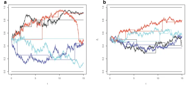
Example 7(PWC martingale on(0,1))Let N be a Poisson process with intensity λandZ˜ be the-martingale(Jeanblanc and Vrins 2018)with constant diffusion coefficientη,
˜ Zt :=
−1(Z0)eη
2/2t
+η
t
0 eη
2
2(t−s)dWs
. (15)
Then, the stochastic process Z defined asZt := ˜Zgt(N ),t ≥ 0, is a pure jump martingale on(0,1)with CDF
FZt(z)=e− λt
!
1{Z0≤z}+λ
t
0
!
−1(z)−−1(Z0)eη
2/2u
eη2u
−1
"
eλudu
"
. (16)
Some sample paths forZ˜andZare drawn on Fig.2. Notice that all the martingales
˜
Zgiven above can be simulated without error using the exact solution.
a b
Fig. 2 (Sample paths ofZ): four sample paths ofZ˜(circles) andZ(no marker) up toT =15 years, where
˜
Figure3gives the CDF ofZandZ˜where the later is a-martingale. The main dif-ferences between these two sets of curves result from the fact thatPZ˜t =Z0
=0
for all t > 0 while P(Zt =Z0) = P
˜
Zgt(N )=Z0
= P(Nt = 0) > 0
and that there is a delay resulting from the fact thatZt correspond to some past
value ofZ˜.
5 Conclusion and future research
Many applications, like mathematical finance, extensively rely on martingales. In this context, discrete- or continuous-time processes are commonly considered. However, in some specific cases like when we work under partial information or when market
a b
c d
Fig. 3
CDF ofZ˜t
: CDF ofZ˜t(circles) andZt(no marker) whereZ˜is the-martingale withZ0=0.5
quotes arrive in a scarce way, it is more realistic to assume that conditional expec-tations move in a more piecewise constant fashion. Such type of processes didn’t receive attention so far, and our paper aims at filling this gap. We focused on the construction of piecewise constant martingales that is, martingales whose trajecto-ries are piecewise constant. Such processes are indeed good candidates to model the dynamics of conditional expectations of random variables under partial (punctual) information. The time-changed approach proves to be quite powerful: starting with a martingale in a given range, we obtain a PWC martingale by using a piecewise constant time-change process. Among those time-change processes,lazyclocks are specifically appealing: these are time-change processes staying always in arrears to the real clock, and that synchronizes to the calendar time at some random times. This ensures thatθt ≤ t which is a convenient feature when one needs to sample
trajec-tories of the time-change process. Such random times can typically be characterized as last passage times, and enjoy appealing tractability properties. The last jump time of a Poisson process before the current time for instance exhibits a very simple dis-tribution. Other lazy clocks have been proposed as well, based on Brownian motions and Bessel processes, some of which rule out the probability mass at zero. We pro-vided several martingales time-changed with lazy clocks (calledlazy martingales) whose range can be any interval inR(depending on the range of the latent martin-gale) and showed that the corresponding distributions can be easily obtained in closed form. Finally, we presented algorithms to sample Poisson and Brownian lazy clocks, thereby providing the reader with a workable toolbox to efficiently use piecewise constant martingales in practice.
This paper paves the way for further research, in either fields of probability theory and mathematical finance. Tractability and even more importantly, the martingale property results from the independence assumption between the latent martingale and the time-change process. It might be interesting however to consider cases where the sample frequency (synchronization rate of the lazy clockθto the real clock) depends on the level of the latent martingaleZ. Finding a tractable model allowing for this coupling remains an open question at this stage. On the other hand, it is yet unclear how dealing with more realistic processes like piecewise constant ones would impact hedging strategies and model completeness in finance. In fact, investigating this route is the purpose of a research project that we are about to initiate.
Abbreviations
CDF: Cumulative distribution function; CIR: Cox–Ingersoll–Ross; PWC: Piecewise constant martingale; PDF: Probability distribution function
Acknowledgements The authors are grateful to M. Jeanblanc, D. Brigo, K. Yano, and G. Zhengyuan for stimulating discussions about an earlier version of this manuscript. We wish to thank the two anonymous referees and the AE whose many suggestions helped to improve the presentation of this paper.
Funding