University of Pennsylvania
ScholarlyCommons
Publicly Accessible Penn Dissertations
2019
Exploiting Cross-Lingual Representations For
Natural Language Processing
Shyam Upadhyay
University of Pennsylvania, [email protected]
Follow this and additional works at:
https://repository.upenn.edu/edissertations
Part of the
Computer Sciences Commons
This paper is posted at ScholarlyCommons.https://repository.upenn.edu/edissertations/3265
Recommended Citation
Upadhyay, Shyam, "Exploiting Cross-Lingual Representations For Natural Language Processing" (2019).Publicly Accessible Penn Dissertations. 3265.
Exploiting Cross-Lingual Representations For Natural Language
Processing
Abstract
Traditional approaches to supervised learning require a generous amount of labeled data for good generalization. While such annotation-heavy approaches have proven useful for some Natural Language Processing (NLP) tasks in high-resource languages (like English), they are unlikely to scale to languages where collecting labeled data is di cult and time-consuming. Translating supervision available in English is also not a viable solution, because developing a good machine translation system requires expensive to annotate resources which are not available for most languages.
In this thesis, I argue that cross-lingual representations are an effective means of extending NLP tools to languages beyond English without resorting to generous amounts of annotated data or expensive machine translation. These representations can be learned in an inexpensive manner, often from signals completely unrelated to the task of interest. I begin with a review of different ways of inducing such representations using a variety of cross-lingual signals and study algorithmic approaches of using them in a diverse set of
downstream tasks. Examples of such tasks covered in this thesis include learning representations to transfer a trained model across languages for document classification, assist in monolingual lexical semantics like word sense induction, identify asymmetric lexical relationships like hypernymy between words in different languages, or combining supervision across languages through a shared feature space for cross-lingual entity linking. In all these applications, the representations make information expressed in other languages available in English, while requiring minimal additional supervision in the language of interest.
Degree Type Dissertation
Degree Name
Doctor of Philosophy (PhD)
Graduate Group
Computer and Information Science
First Advisor Dan Roth
Keywords
cross-lingual, low supervision, multilingual, natural language processing, representation learning
EXPLOITING CROSS-LINGUAL REPRESENTATIONS FOR NATURAL LANGUAGE PROCESSING
Shyam Upadhyay
A DISSERTATION
in
Computer and Information Science
Presented to the Faculties of the University of Pennsylvania
in
Partial Fulfillment of the Requirements for the
Degree of Doctor of Philosophy
2019
Supervisor of Dissertation
Dan Roth, Professor of Computer and Information Science
Graduate Group Chairperson
Rajeev Alur, Professor of Computer and Information Science
Dissertation Committee
Adam Kalai, Principal Researcher, Microsoft Research
Chris Callison-Burch, Professor of Computer and Information Science
Lyle Ungar, Professor of Computer and Information Science
EXPLOITING CROSS-LINGUAL REPRESENTATIONS
FOR NATURAL LANGUAGE PROCESSING
© COPYRIGHT
2019
Shyam Upadhyay
This work is licensed under the
Creative Commons Attribution
NonCommercial-ShareAlike 3.0
License
To view a copy of this license, visit
ACKNOWLEDGEMENT
Nothing of me is original. I am the combined
effort of everybody I’ve ever known.
Chuck Palahniuk, Invisible Monsters
Very few Ph.D. students get the opportunity of working with a great advisor like Dan.
Without his continuous support, patience and his open style of advising that grants research
freedom, most of the work in this thesis would not have seen the light of day. Besides being a
great advisor, Dan is one of the kindest and most considerate person I know. I am immensely
grateful for all that he has done for me. I am also indebted to my thesis committee — Adam,
Mitch, Lyle, and Chris. Not only have they provided valuable feedback on the thesis at
various stages, but also have been a source of sage advice.
During my Ph.D., I also got the valuable opportunity to work with some of the best
re-searchers in the field through internships at Microsoft Research and Google. Working with
Ming-Wei and Scott was instrumental in shaping my thinking and temperament for
re-search. The wisdom I got from Ming-Wei will be invaluable for the rest of my research life.
The next summer at MSR Cambridge was equally enjoyable, where Adam, Matt, Kai-Wei,
and James gave me the freedom to define and work on a research problem, and helping
me find a way towards a solution. Lastly, the summer spent working with Gokhan, Dilek
and Larry taught me how to approach problems outside my comfort zone, and keeping in
mind practical considerations when thinking about new ideas. I am thankful for all these
experiences, which have shaped my outlook and approach towards research.
I would like to thank former and current members of CogComp — especially Mark Sammons,
Kai-Wei Chang, Rajhans Samdani, and Gourab Kundu, who helped me fit in the group in
my early days. Working in CogComp also brought me in contact with Christos, Parisa,
Michael, Snigdha, and Wenpeng, who took the trouble of mentoring me when they were
giving me research advice at different stages of my Ph.D., and constantly reminding me
“not to work too hard over the weekends”. I am also indebted to Yangqiu Song, who really
did all the hard work that later became Chapter 4. Special thanks to Snigdha, who was
influential in helping me frame the early draft of this thesis.
During my stay at UIUC and UPenn, I developed close friends in brilliant fellow students
like Subhro, Haoruo, Nitish, Daniel, John, Chen-Tse, Stephen, Dan (Deutsch), Qiang, Anne,
Jordan, Reno, João, Daphne, and others. When I reflect how much I have learned from all
of you over the years, it amazes me. I am sure you will have prolific and satisfying careers
ahead of you. I will dearly miss the discussions over lunches and happy hours we had. I
will especially miss the evening meals I had with Subhro, Nitish, Snigdha, and Shashank.
The not-so-good Indian food in the US will taste even worse without your company.
I would be remiss in not thanking my remote collaborators — Manaal, Chris (Dyer),
Yo-garshi, and Marine. Working with all of you was a unique experience and I have acquired
countless skills and research wisdom from our interactions. Special thanks to Manaal, who
I often trouble for research and career advice from time to time.
It would be unfair not to thank the folks behind the scenes who ensure things run smoothly
in CogComp at UIUC and UPenn. Thanks to Dawn Cheek, Eric Horn and Jennifer Sheffield,
who often went out of their way to help students like me.
Lastly, I would like to thank Maa, Papa and everyone in my family whose efforts and
sacrifices got me here. Thanks for your unconditional love and support when things were not
going well, and uplifting my spirits when I was facing the despair that naturally accompanies
ABSTRACT
EXPLOITING CROSS-LINGUAL REPRESENTATIONS
FOR NATURAL LANGUAGE PROCESSING
Shyam Upadhyay
Dan Roth
Traditional approaches to supervised learning require a generous amount of labeled data for
good generalization. While such annotation-heavy approaches have proven useful for some
Natural Language Processing (NLP) tasks in high-resource languages (like English), they are
unlikely to scale to languages where collecting labeled data is difficult and time-consuming.
Translating supervision available in English is also not a viable solution, because developing
a good machine translation system requires expensive to annotate resources which are not
available for most languages.
In this thesis, I argue that cross-lingual representations are an effective means of extending
NLP tools to languages beyond English without resorting to generous amounts of annotated
data or expensive machine translation. These representations can be learned in an
inexpen-sive manner, often from signals completely unrelated to the task of interest. I begin with a
review of different ways of inducing such representations using a variety of cross-lingual
sig-nals and study algorithmic approaches of using them in a diverse set of downstream tasks.
Examples of such tasks covered in this thesis include learning representations to transfer a
trained model across languages for document classification, assist in monolingual lexical
se-mantics like word sense induction, identify asymmetric lexical relationships like hypernymy
between words indifferent languages, or combining supervision across languages through a
shared feature space for cross-lingual entity linking. In all these applications, the
represen-tations make information expressed in other languages available in English, while requiring
Contents
ACKNOWLEDGEMENT . . . iv
ABSTRACT . . . vi
LIST OF TABLES . . . xviii
LIST OF ILLUSTRATIONS . . . xxiii
CHAPTER 1 : Introduction . . . 1
1.1 Overview . . . 1
1.2 Thesis Statement . . . 4
1.3 Outline of This Thesis . . . 4
CHAPTER 2 : History of Word Representations . . . 7
2.1 Introduction . . . 7
2.2 One-Hot Word Representations . . . 7
2.3 Distributional Semantics . . . 8
2.4 Cluster-based Word Representations . . . 11
2.5 Vector-based Word Representations . . . 13
2.6 Sparse Word Representations using Count Models . . . 15
2.7 Dense Word Representations using Exact Matrix Factorization . . . 17
2.8 Dense Word Representations using Neural Language Modeling . . . 19
2.9 Dense Word Representations using Approximate Matrix Factorization . . . 20
2.10 Limitations of Word Representations . . . 23
CHAPTER 3 : Cross-lingual Word Representations . . . 26
3.1 Introduction . . . 26
3.3 Cluster-based Cross-lingual Representations . . . 28
3.4 Vector-based Cross-lingual Representations . . . 29
3.4.1 Sentence and Word-level Alignment . . . 30
3.4.2 Sentence-level Alignment . . . 31
3.4.3 Word-level Alignment . . . 32
3.4.4 Document-level Alignment . . . 33
3.5 Experiments . . . 34
3.5.1 Monolingual Lexical Similarity . . . 35
3.5.2 Cross-lingual Dictionary Induction . . . 37
3.5.3 Cross-lingual Document Classification . . . 38
3.5.4 Cross-lingual Dependency Parsing . . . 40
3.6 Summary . . . 42
CHAPTER 4 : Deriving Cross-lingual Representations from Wikipedia . . . 43
4.1 Introduction . . . 43
4.2 Background . . . 43
4.2.1 Explicit Semantic Representations (ESA) . . . 43
4.2.2 Dataless Document Classification using ESA . . . 46
4.3 Inter-lingual Structure of Wikipedia . . . 47
4.4 Cross-lingual ESA (CLESA) . . . 48
4.5 Experimental Setup and Experiments . . . 50
4.5.1 CLESA v/s Supervised Classification . . . 50
4.5.2 CLESA v/s Monolingual ESA . . . 51
4.6 Summary . . . 52
CHAPTER 5 : Multi-sense Representation Learning with Cross-lingual Signals . . 54
5.1 Introduction . . . 54
5.2 Related Work — Representing Word Senses . . . 55
5.2.2 Data-driven Sense Representations . . . 57
5.2.3 Motivation for Our Work . . . 58
5.3 Model Description . . . 59
5.4 Learning and Disambiguation . . . 62
5.5 Multilingual Extension . . . 64
5.6 Experimental Setup . . . 65
5.7 Experiments . . . 67
5.7.1 Word Sense Induction (WSI) Results . . . 67
5.7.2 Effect of Language Family Distance . . . 68
5.7.3 Effect of Window Size . . . 69
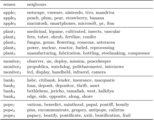
5.7.4 Qualitative Analysis of Induces Senses . . . 70
5.8 Summary . . . 71
CHAPTER 6 : Identifying Hypernymy across Languages . . . 73
6.1 Introduction . . . 73
6.2 History of the Hypernymy Detection Task . . . 73
6.2.1 Hypernymy Detection in English . . . 74
6.2.2 Cross-lingual Hypernymy Detection . . . 75
6.3 The BiSparse-DepApproach . . . 76
6.4 Crowd-Sourcing Annotations . . . 81
6.5 Experimental Setup . . . 84
6.6 Experiments . . . 87
6.6.1 Dependency v/s Window Contexts . . . 87
6.6.2 Ablating Directionality in Context . . . 89
6.6.3 Qualitative Analysis . . . 90
6.7 Evaluating Robustness ofBiSparse-Dep . . . 91
6.7.1 No Treebank . . . 91
6.7.2 Small Monolingual Corpus . . . 93
6.7.4 Choice of Hypernymy Detection Measure . . . 94
6.8 Summary . . . 94
CHAPTER 7 : Multilingual Supervision for Cross-lingual Entity Linking . . . 96
7.1 Introduction . . . 96
7.2 History of the Entity Linking Task . . . 97
7.2.1 Monolingual Entity Linking . . . 98
7.2.2 Cross-lingual Entity Linking . . . 101
7.2.3 Our Work . . . 103
7.3 Cross-lingual EL with Xelms . . . 105
7.3.1 Mention Context Representation . . . 105
7.3.2 Including Type Information . . . 108
7.4 Training and Inference . . . 109
7.4.1 Candidate Generation . . . 109
7.4.2 Inference . . . 110
7.4.3 Training Objective . . . 111
7.5 Experimental Setup . . . 111
7.6 Experiments . . . 114
7.6.1 Monolingual and Joint Models . . . 115
7.6.2 Multilingual Training . . . 116
7.6.3 Adding Fine-grained Type Information . . . 117
7.7 Experiments with Limited Resources . . . 117
7.7.1 Zero-shot Setting . . . 118
7.7.2 Low-resource Setting . . . 120
7.8 Summary . . . 121
CHAPTER 8 : Bootstrapping Transliteration with Constrained Discovery . . . 123
8.1 Introduction . . . 123
8.2.1 Transliteration Generation . . . 125
8.2.2 Transliteration Discovery . . . 126
8.2.3 Our Work . . . 127
8.3 Transliteration with Hard Monotonic Attention . . . 128
8.4 Low-Resource Bootstrapping . . . 130
8.4.1 The Bootstrapping Algorithm . . . 131
8.4.2 Discovery Constraints . . . 131
8.5 Experimental Setup . . . 132
8.6 Experiments . . . 134
8.6.1 Full Supervision Setting . . . 134
8.6.2 Low-Resource Setting . . . 136
8.6.3 Error Analysis . . . 137
8.7 Challenges Inherent to Transliteration . . . 137
8.7.1 Source and Target-Specific Issues . . . 138
8.7.2 Disparity between Native and Foreign . . . 139
8.8 Case Studies . . . 139
8.8.1 Manual Annotation . . . 140
8.8.2 Candidate Generation . . . 142
8.9 Summary . . . 144
CHAPTER 9 : Conclusion . . . 146
9.1 Summary of Contributions . . . 146
9.2 Future Directions . . . 150
APPENDIX . . . 152
A.1 Statistical Measures used in the Thesis . . . 152
A.2 BiSparse — Bilingual Sparse Coding . . . 155
A.3 Qualitative Analysis for Multi-sense Embeddings . . . 155
List of Tables
TABLE 1 : The distributional hypothesis in action: We (humans) can guess the
meaning of words likewampimuk by the context in which it appears. 8
TABLE 2 : Example of a word-context co-occurrence matrix extracted from a
corpus. Each dimension of a row corresponds to co-occurrence with
a certain context word. For instance, the word apple co-occurs with
fruit (4th dimension) 20 times in the corpus. . . . 14
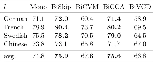
TABLE 3 : Word similarity score measured in Spearman’s correlation ratio for
English on SimLex-999. The best score for each language pair is
shown in bold. Scores that are significantly better (per Steiger’s
Method with p <0.1) than the next lower score are underlined. For
example, for English-Chinese, BiCVM is significantly better than
BiSkip, which in turn is significantly better than BiVCD. . . 36
TABLE 4 : Intrinsic evaluation of English word vectors measured in terms of
Qvec score across models. Best scores for each language pair is
shown in bold. . . 37
TABLE 5 : Cross-lingual dictionary induction results (top-10 accuracy). The
same trend was also observed across models when computing MRR
TABLE 6 : Cross-lingual document classification accuracy when trained on
lan-guage l1, and test on language l2. Best scores for each language is
shown inbold. Majority baselines for English→l2andl1→English
are 49.7% and 46.7% respectively, for all languages. Scores
signif-icantly better (per McNemar’s Test, p < 0.05) than the next best
score are underlined. For example, for Swedish → English, BiVCD
is significantly better than BiSkip, which is significantly better than
BiCVM. . . 39
TABLE 7 : Labeled attachment score (LAS) for dependency parsing when trained
and tested on language l (direct-parsing experiment). Mono refers
to parser trained with mono-lingually induced embeddings. Scores
inboldare better than the Mono scores for each language, showing
improvement from cross-lingual training. . . 40
TABLE 8 : Labeled attachment score (LAS) for cross-lingual dependency
pars-ing when trained on languagel1, and evaluated on languagel2
(model-transfer experiment). The best score for each language is shown in
bold. . . 41
TABLE 9 : Concept-term matrix constructed using the English Wikipedia.
Ex-plicit Semantic Analysis (ESA) representations are derived from the
matrix above by reweighing each entry using TF-IDF and
normal-izing the columns. Each column describes a word in English using a
“bag-of-concepts” in Wikipedia. . . 44
TABLE 10 : Statistics showing number of articles in Wikipedias for 9 languages,
and the size of the intersection (as identified by inter-language links)
with the English Wikipedia. The last column shows the relative
size of the intersection (in % age). For instance, 52% of German
TABLE 11 : Concept-term matrix constructed using the English, Spanish and
Hindi Wikipedias (compare to Table 9). From left to right, the words
in Spanish and Hindi translate to tower, big, politician, olympic,
democratic, hawaii respectively. The term counts are computed in
the respective article in the Spanish or Hindi Wikipedia. CLESA
representations are derived from this matrix by weighing each entry
using TF-IDF and normalizing the columns. Each column describes
a word using a “bag-of-concepts” in Wikipedia. . . 49
TABLE 12 : Comparing monolingual ESA (Mono) and cross-lingual ESA (CLESA)
for classification on translated documents from 20-Newsgroup. The
table shows the number of languages which achieve accuracies in a
certain range with a given ESA representation (Mono or CLESA).
For instance, CLESA achieves accuracy@1 in the range of 70% to
80% (i.e.,0.8> p≥0.7) for 7 languages. It can be seen that CLESA
achieves high accuracies (e.g., accuracy@1 lies in 1 ≥ p ≥ 0.9) for
20 languages, whereas the same is true for monolingual ESA for 2
languages only. . . 52
TABLE 13 : Corpus statistics (in millions) of the parallel corpora used to train
the multi-sense representations. Horizontal lines demarcate corpora
from the same domain. . . 66
TABLE 14 : Results on word sense induction (left four columns) in ARI and
con-textual word similarity (last column) in percent correlation.
Lan-guage pairs are separated by horizontal lines. Best results inbold. 67
TABLE 15 : Effect (in ARI) of language family distance on WSI task. Best results
for each column is shown in bold. The improvement from Mono
to Full is shown as (3) - (1). Note that this is not comparable to
results in Table 14, as a different training corpus is used to control
TABLE 16 : Senses discovered for some words under multilingual training, and
their nearest neighbors in the vector space. . . 70
TABLE 17 : Crowd-sourced dataset statistics. #pos (#neg) denote the number
of positives (negatives) in the evaluation set, and #crowd-sourced
denote the number of crowd-sourced pairs. Negatives were
deliber-ately under-sampled to have a balanced evaluation set. Some
exam-ples for positive and negative instances in French and Russian are:
(pêcheur (en:fisher), worker) (vêtement (en:clothing), jeans) (замок
(en:castle), structure) (флора(en:flora), sunflower) . . . 83
TABLE 18 : Training data statistics for different languages. While we use parallel
corpora for computing translation dictionaries, our approach can
work with any bilingual dictionary. . . 85
TABLE 19 : Comparing the different approaches from Section 6.5 with our
BiSparse-Dep approach onHyper-Hypo(random baseline= 0.5). Bold
de-notes the best score for each language, and the * on the best score
indicates a statistically significant (p< 0.05) improvement over the
next best score, using McNemar’s test (McNemar, 1947). . . 88
TABLE 20 : Comparing the different approaches from Section 6.5 with our
BiSparse-Dep approach on Hyper-Cohypo (random baseline= 0.5). Bold
denotes the best score for each language, and the * on the best score
indicates a statistically significant (p< 0.05) improvement over the
next best score, using McNemar’s test (McNemar, 1947). . . 88
TABLE 21 : Common errors made by the different models described in Section 6.3. 90
TABLE 22 : Robustness to absence of a treebank: The delexicalized model
is competitive to the best dependency based and the best window
based models on both test sets. For each dataset, * indicates a
statistically significant (p < 0.05) improvement over the next best
TABLE 23 : Part of a dictionary compiled from Wikipedia hyperlinks showing the
entities that the stringchicagocan refer to, along with the respective
prior probabilities and counts. . . 99
TABLE 24 : Number of train mentions (from Wikipedia) in each language, with
% size relative to English (51.7M mentions). Train mentions from
Wikipedias like Arabic, Turkish and Tamil are <10% the size of
those from the English Wikipedia. . . 112
TABLE 25 : Evaluation datasets used in the cross-lingual entity linking
experi-ments. . . 113
TABLE 26 : Xelms(joint) improves upon Xelms(mono) and the current
State-of-The-Art (SoTA) onTH-TestandMcN-Test, showing the
ben-efit of using additional supervision from English. The best score
is shown bold and ∗ marks statistical significance of best against
SoTA. Refer Section 7.5 for details on SoTA. . . 115
TABLE 27 : Linking accuracy on TAC15-Test. Numbers for Sil et al. (2018) from
personal communication. . . 116
TABLE 28 : Linking accuracy of asingleXelms(multi) model for four languages
— German, Spanish, French and Italian. For comparison,
individ-ually trained Xelms(joint) scores are also shown. The best score
is shown bold and ∗ marks statistical significance of best against
SoTA. Refer Section 7.5 for details on SoTA. . . 116
TABLE 29 : Adding fine-grained type information further improves linking
ac-curacy (compare to Table 26). The best score is shown bold and ∗
marks statistical significance of best against SoTA. Refer Section 7.5
TABLE 30 : Linking accuracy of the zero-shot (Z-S) approach on different datasets.
Zero-shot (w/ prior) is close to SoTA for datasets like TAC15-Test,
but performance drops in the more realistic setting of zero-shot (w/o
prior) (Section 7.7.1) on all datasets, indicating most of the
perfor-mance can be attributed to the presence of prior probabilities. The
slight drop in McN-Test is due to trivial mentions that only have
a single candidate. . . 119
TABLE 31 : Cumulative number of person name pairs in Wikipedia inter-language
links. For instance, 45 languages (that cover 22 scripts) have at least
1000 name pairs that can be extracted from inter-language links.
While previous approaches for transliteration generation were
appli-cable to only 24 languages (spanning 15 scripts), our approach is
applicable to 56 languages (23 scripts). When counting scripts we
exclude variants (e.g., all Cyrillic scripts and variants count as one). 127
TABLE 32 : Comparing different generation approaches on the NEWS 2015 dataset
using accuracy@1 as the evaluation metric for five languages —
Hindi (hi), Kannada (kn), Bengali (bn), Tamil (ta) and Hebrew
(he) – in full supervision and low-resource settings. “Ours” denotes
the Seq2Seq(HMA) model, with (.) denoting the inference strategy.
The rest of the approaches are described in Section 8.5. Numbers
for RPI-ISI are from Lin et al. (2016). . . 135
TABLE 33 : Accuracy@1 for native and foreign words for four languages
(Sec-tion 8.7.2). Ratio is native performance relative to foreign. . . 140
TABLE 34 : Corpora used for obtaining foreign vocabularyVf for bootstrapping
TABLE 35 : Accuracy@1 of Seq2Seq(HMA) model supervised using human
an-notated seed set in Punjabi and Armenian (with and without
boot-strapping). Both languages perform well relative to the other
lan-guages investigated so far. Both annotation sub-tasks took roughly
the same time. . . 141
TABLE 36 : Comparing candidate recall@20 for different approaches on Tigrinya
and Macedonian. CV-split refers to consonant-vowel splitting. Using
our transliteration generation model with bootstrapping yields the
List of Figures
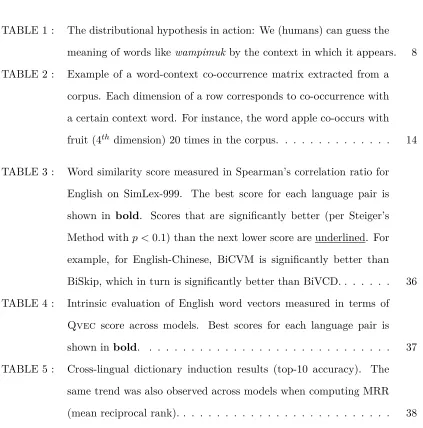
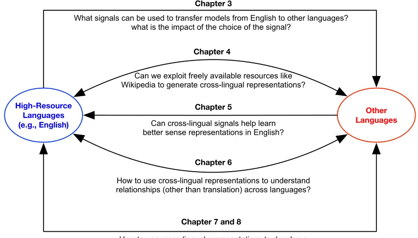
FIGURE 1 : Overview of the chapters in this thesis. The double-headed arrows
indicate tasks involving sharing of information between languages,
and single-headed arrows indicate tasks involving transfer from one
language to another. . . 5
FIGURE 2 : Vector-based word representations in a 2-dimensional space. . . . 14
FIGURE 3 : Cross-lingual word representations as a vector space
approxima-tion of discrete translaapproxima-tion dicapproxima-tionaries. By encoding items present
in the dictionary as points in a continuous vector space, one can
recover some of the missing entries. Note that while the figure uses
vector-based representations (which partition the space implicitly)
a similar reasoning can be applied to cluster-based representations
(which partition the space explicitly). . . 27
FIGURE 4 : Different forms of cross-lingual alignments one can use as
supervi-sion for learning cross-lingual representations. From left to right,
the cost of the supervision required varies from expensive (sentence
and word-level alignments) to cheap (document-level alignment). . 29
FIGURE 5 : Inter-language links in English Wikipedia and Hindi Wikipedia link
the corresponding articles that describe the entityAlbert_Einstein
in both Wikipedias. . . 47
FIGURE 6 : Comparing CLESA based document classification with supervised
classification on the TED dataset (averaged macro-F1 scores over
15 labels) for 7 languages — English (en), Arabic (ar), German
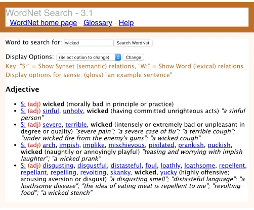
FIGURE 7 : Senses listed in WordNet for the word wicked when used as an
adjective. None of the senses listed reflect the sense of wicked in
the sentence, “Tony Hawk did a wicked ollie at the convention”,
wherewicked is used as an adjective denoting awesome-ness. . . . 56
FIGURE 8 : Benefit of Multilingual Information (beyond bilingual): Two
different senses of the wordinterestand their translations to French
and Chinese (word translation shown in [bold]). While the
sur-face form of both senses of interest are same in French, they are
different in Chinese, illustrating the benefit of having more than
two languages. . . 59
FIGURE 9 : The aligned pair (interest,intérêt) is used to predict monolingual
and cross-lingual context in both languages (see factors in
Equa-tion (5.7)). Each sense vector (here 2nd is shown) for interest,
participates in the update. Only the polysemy in English is
mod-elled. . . 61
FIGURE 10 : Tuning window size for English-Chinese and English-French models. 69
FIGURE 11 : The BiSparse-Dep Approach, that learns sparse bilingual
em-beddings using dependency-based contexts. The resulting sparse
embeddings, together with an unsupervised hypernymy detection
measure, can detect hypernyms across languages (e.g.,pomme is a
fruit). . . . 77
FIGURE 12 : Dependency tree for “The tired traveler roamed the sandy desert,
seeking food”. . . . 77
FIGURE 13 : Robustness to small corpus: For most languages,
BiSparse-Depoutperforms the corresponding best window based model on
FIGURE 14 : Robustness to low quality dictionary: For most languages,
BiSparse-Depoutperforms the corresponding best window based
model onHyper-Hypo, with increasingly lower quality dictionaries. 93
FIGURE 15 : Tamil and English mention contexts containing [mentions] of the
entity Liverpool_F.C. from the respective Wikipedias. Tamil
Wikipedia only has 9 mentions referring toLiverpool_F.C., whereas
English Wikipedia has 5303 such mentions. Clearly, there is a
need to augment the limited contextual evidence in low-resource
languages (like Tamil) with evidence from high-resource languages
(like English). The Tamil sentence translates to “Suarez plays for
[Liverpool] and Uruguay.” . . . 101
FIGURE 16 : (a) Xelms uses grounded mentions from two or more languages
(English and Tamil shown) as supervision. The contextg, entity
e and type t vectors interact through Entity-Context loss (
EC-Loss), Type-Context loss (TC-Loss) and Type-Entity loss (
TE-Loss). The Tamil sentence is the same as in Figure 15, and other
mentions in it translate to [Suarez] and [Uruguay]. (b) The
Mention Context Encoder (Section 7.3.1) encodes the local
con-text (neighboring words) and the document concon-text (surfaces of
other mentions in the document) of the mention into g. Internal
view of local context encoder is in Figure 17. . . 104
FIGURE 17 : Local Context Encoder, for the right context. Figure 16b shows
how it fits inside Mention Context Encoder. . . 107
FIGURE 18 : Candidate generation using inter-language links in Wikipedia. Prior
probabilities are computed from surface to index statistics
FIGURE 19 : Linking accuracy v/s the number of train mentions in the target
language L (= Turkish (tr), Chinese (zh) and Spanish (es)). We
compare bothXelms(mono) and Xelms(joint) to the best results
using all available supervision, denoted by L-best. To discount the
effect of the prior, all results above are without it. For number of
train mentions = 0,Xelms(joint) is equivalent to zero-shot without
prior. Best viewed in color. . . 120
FIGURE 20 : Limitation of the candidate generation approach described in
Fig-ure 18. For the Russian mention (that transliterates to Berlin),
using inter-language links misses two plausible candidate entities
in the English Wikipedia. . . 123
FIGURE 21 : Generation treats transliteration as a sequence transduction task,
while discovery aims to select the correct transliteration from a
given list of names. . . 125
FIGURE 22 : Transliteration using Seq2Seq transduction with Hard Monotonic
Attention, or Seq2Seq(HMA). The figure shows how decoding
pro-ceeds for transliterating थनोस to thanos. During decoding, the
model attends to a source character (e.g.,थ shown in blue) and
outputs target characters (t,h,a) until astep action is generated,
which moves the attention position forward by one character (to
न), and so on. . . 129
FIGURE 23 : Plot showing accuracy@1 after each bootstrapping iteration for
Hindi, Kannada, Bengali, Tamil and Hebrew, starting with only
500 training pairs as supervision. For comparison, the accuracy@1
of a model trained with all available supervision is also shown
FIGURE 24 : Summary of contributions made in the thesis. Different chapters
demonstrated how cross-lingual representations can help achieve
model transfer and sharing (Chapter 3 and 4), aid in lexical
se-mantics tasks either monolingually (Chapter 5) or cross-lingually
(Chapter 6), and facilitate cross-lingual information extraction
(Chap-ter 7 and 8). . . 147
FIGURE 25 : PCA plots for the vectors for {apple, bank, interest, itunes, potato,
west, monetary, desire}with multiple sense vectors for apple
(ap-ple_1and apple_2),interest(interest_1and interest_2) andbank
(bank_1 and bank_2) obtained using monolingual (25a), bilingual
CHAPTER 1 : Introduction
1.1. Overview
Most work in Natural Language Processing (NLP) is driven by the availability of supervision
in the form of labeled data. Such labeled data is relatively easily available for simple
NLP tasks in high-resource languages (like document classification for English), but this
is not true for other languages. In fact, for more sophisticated NLP tasks like semantic
parsing, fully labeled data is hard to come by even in English, let alone other languages.
Consequently, even though there are over 7000 languages from over 140 different language
families in use across the world (Lewis, 2009), the state of NLP is skewed towards
high-resource languages like English.
Why should one care about NLP in other languages? Developing NLP technology that can
operate multilingually has several benefits. A large population of the world is multilingual,
and produces information at a unprecedented scale across several languages thanks to the
web. Indeed, over 40% of the content on the web is not in English, and the rate at which
such content is generated has been growing dramatically.1 Although most of this content is
publicly available (online news, social media platforms etc.), yet consuming it is complicated
by the multitude of languages used. Multilingual NLP makes this information available to
a broader audience than what the language in which it was expressed can reach, helping
overcome the metaphorical language-imposed barrier to knowledge. For instance, knowing
what entities appear in a certain tweet written in Hindi can improve the understanding of an
English reader. This can help faster dissemination of critical information, that can prove
crucial in urgent situations (e.g., early warning systems, financial trading). Multilingual
NLP can also help from a scientific standpoint, in understanding how languages evolve and
interact with each other, revealing previously unknown similarities or differences between
languages (Bender, 2009, 2011).
Unfortunately, traditional supervised learning approaches, which form the backbone of
cur-rent NLP technology, are inhecur-rently ill-equipped to deal with the lack of labeled data, which
poses a significant challenge in scaling to other languages. As a result, advances made in
NLP for high-resource languages take longer to percolate to the rest of the languages. To
bridge this language barrier, efforts have been made in two directions.
Annotation-heavy Approaches. The first direction is motivated by the overwhelming
success of supervised machine learning approaches for English NLP tasks. Given enough
training data, traditional machine learning approaches have shown remarkable
generaliza-tion abilities. One natural step is to apply these approaches to NLP tasks in non-English
lan-guages, by providing supervision in the target language. Often, such supervision is derived
from multilingual resources that are used in machine translation, such as parliamentary
pro-ceedings (Koehn, 2005) or translations of the Bible (Christodouloupoulos and Steedman,
2015; Agić et al., 2015). A popular approach for achieving this is annotation projection,
where annotation for some linguistic structure is projected from a high resource language to
a low resource language, usually by means of some cross-lingual alignment (Yarowsky and
Ngai, 2001; Hwa et al., 2005). Nevertheless, the community has also invested in curating
an-notated resources in non-English languages for various NLP tasks (Xue, 2008; de Melo and
Weikum, 2009; McDonald et al., 2013), so that traditional supervised learning approaches
can be developed for these languages. Indeed, statistical machine learning approaches have
become integral to advancing NLP in English in past three decades, and it is reasonable
to assume that they will succeed for other languages once the appropriate datasets become
available.
Translation-based Approaches. The second direction has advocated extending NLP
to languages other than English by automatically translating text in the target language
to English using machine translation, and then using state-of-the-art NLP models already
developed for English. Like annotation-heavy approaches, this direction also relies on the
translation from a language to English will be sufficient to bridge the language barrier.
In-deed, translation quality from a non-English language to English has improved considerably
over the past few years with the advent of neural machine translation (Sutskever et al., 2014;
Bahdanau et al., 2015; Luong et al., 2015a; Sennrich et al., 2016, inter alia).
While promising, both of these directions suffer from limitations. Traditional supervised
learning approaches require generous amount of labeled data to achieve good generalization.
While such annotation-heavy approaches have proved successful for high resource languages
such as English, their applicability to a new language is limited due to lack of labeled data.
Collecting high-quality labelled data for any NLP task in an arbitrary language is
chal-lenging due to the human effort involved and the paucity of expert annotators. There are
practical limitations as well — generating high-quality annotations such as treebanks
(Mar-cus et al., 1993; Prasad et al., 2008; McDonald et al., 2013; Socher et al., 2013) takes time
and expertise. This may not be ideal if one has limited time to develop a system in a
language to achieve certain goals (e.g., for disaster management).
Similar problems affect machine translation. Building a translation system requires
re-sources in the target language (namely large parallel corpora with English), which are not
always available and are expensive to annotate at scale (Lopez and Post, 2013). Unless
several million lines of in-domain parallel text are available, statistical machine translation
approaches perform poorly (Kolachina et al., 2012; Irvine, 2014), an issue that is
exacer-bated for the now popular neural machine translation approaches (Koehn and Knowles,
2017). From a practical standpoint too, including a translation system in the pipeline may
prove to be an overkill for simple understanding tasks such document classification. For
instance, knowing thatगु वाकषणmeansgravityand वांटम यां क meansquantum mechanics
is sufficient to realize a Hindi document containing the above words is about physics,
with-out translating the entire document. Another practical issue is that even though we can
apply NLP tools on the translated text, often the output is desired in the target language
approach incurs the additional cost of projecting the output back to the original language,
which besides introducing latency, might be a hard task in itself. For instance, how to
project back the Part-Of-Speech (POS) tags for tokens in a English phrase that aligns to a
single word in Hindi?
All the above challenges become more acute when working with low-resource languages. To
extend NLP tools to languages beyond English, we need to find approaches that eliminate
or reduce the dependence on high quality annotated data, and that enable one to scale to
multiple languages quickly without investing too much effort.
1.2. Thesis Statement
In this thesis, I argue thatcross-lingual representationsare an effective means of extending
NLP tools to languages beyond English, without resorting to generous amounts of annotated
data or expensive machine translation. These cross-lingual representations encode semantics
and maintain similarity of lexical items across multiple languages. Such
multilingually-enriched semantic representations can be learnt in an inexpensive manner, often from
cross-lingual signals completely unrelated to the task of interest. By using these representations as
features (in lieu of monolingually derived representations) for training a model for a certain
NLP task, we can learn models that operate on input from multiple languages. Using such
language-agnostic feature representations in the model enable us to leverage any existing
annotations in a high-resource language for joint multilingual training, thereby reducing
the amount of supervision required for the task in a new language.
1.3. Outline of This Thesis
The rest of the document is organized as follows.
• Chapter 2 gives a brief history of different approaches of representing words in NLP
applications, and highlights their limitations in capturing cross-lingual semantics.
limi-High-Resource Languages (e.g., English)
Other Languages What signals can be used to transfer models from English to other languages?
what is the impact of the choice of the signal?
Can we exploit freely available resources like Wikipedia to generate cross-lingual representations?
Can cross-lingual signals help learn better sense representations in English?
How to use cross-lingual representations to understand relationships (other than translation) across languages?
How to use cross-lingual representations to develop a cross-lingual information extraction system?
Chapter 3
Chapter 7 and 8 Chapter 6 Chapter 4
Chapter 5
Figure 1: Overview of the chapters in this thesis. The double-headed arrows indicate tasks involving sharing of information between languages, and single-headed arrows indicate tasks involving transfer from one language to another.
tation, and motivates them as an effective way of translating feature spaces. I then
describe different cross-lingual signals that we can exploit to learn cross-lingual
repre-sentations and evaluate their suitability for achieving semantic and syntactic transfer.
Based on (Upadhyay et al., 2016).
• In Chapter 4, I describe another approach to learn cross-lingual representations using
multilingual encyclopedic resources such as Wikipedia to encode words in different
languages in a shared semantic space, and use it to classify documents without any
supervision. Based on (Song et al., 2016).
• In Chapter 5, I describe our work on learning multi-sense representations in English
using cross-lingual signals, where we show that using a small amount of multilingual
data we can train models for sense induction that compare favorably with a model
• Chapter 6 shows how, by using appropriate cross-lingual word representations, one
can detect asymmetric relations across languages. The chapter demonstrates that
cross-lingual representations can aid in semantic tasks beyond those requiring coarse
semantics (such as document classification). Based on (Upadhyay* et al., 2018).
The next two chapters examine a downstream information extraction task, namely
cross-lingual entity linking, along two dimensions.
• Chapter 7 describes how we can exploit cross-lingual representations to develop a
cross-lingual entity linking system. In particular, I describe how we can augment the
limited supervision in a low-resource language with supervision from a high-resource
language by using a shared multilingual representation space. Based on (Upadhyay
et al., 2018a).
• Chapter 8 examines the problem of name transliteration from a language to English,
a crucial component for performing entity linking in the cross-lingual setting. I show
that we can improve transliteration from low-resource languages into English using
constraints to drive learning with limited supervision. Based on (Upadhyay et al.,
2018b).
Finally, Chapter 9 summarizes the contributions of this thesis and provides an overview of
CHAPTER 2 : History of Word Representations
2.1. Introduction
The generalizability of any machine learning model is a function of the data representation
(or features) that it operates on to make predictions. For instance, the generalizability of a
document classifier depends on what features are used to represent a document. For most
NLP applications, features of smaller units of language such as words are used to derive
features for larger linguistic structures such as sentences and documents. For instance, a
common choice of word-level features in the document classification task is “how often did
word w appear in the document”, and the document-level feature is simply the sum of all
the active word-level features in that document. The choice of feature representation for
units such as words is thus a crucial decision when developing a NLP model.
The idea of learning mathematical representations useful for building classifiers is a general
one (Bengio et al., 2013), and the aim of this chapter is to review different approaches
of representing words as mathematical objects in NLP. The techniques and principles
in-troduced in this chapter for training monolingual representations will serve as the starting
point for cross-lingual representation learning approaches described in the rest of the thesis.
I start with a discussion of one-hot word representations and their limitations. I will then
discuss how the principles of distributional semantics can be put into practice to derive
cluster-based or based word representations. Owing to the popularity of
vector-based representations, I will briefly discuss the different frameworks for learning vector
representations and their benefits. I end the chapter by discussing some known limitations
of these word representations, that I will address in the rest of the thesis.
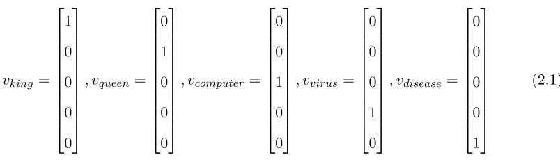
2.2. One-Hot Word Representations
Conventional approaches represent each word w in the vocabulary V by denoting w by
disease}, the one-hot representations will be {1, 2, 3, 4, 5}. This representation scheme is
better visualized by treating each word as a vector of 0s with a 1 at the index associated
with the word (or aone-hot vector),
vking =
1 0 0 0 0
, vqueen =
0 1 0 0 0
, vcomputer=
0 0 1 0 0
, vvirus =
0 0 0 1 0
, vdisease =
0 0 0 0 1 (2.1)
It is easy to see that this is an extremely crude representation that fails to capture
relation-ships (or lack thereof) between words. For instance, related words like king and queen are
treated the same (twodistinct atomic symbols), and so are unrelated words like computer
and king. Using features built on top of one-hot word representations will also suffer from
the same problem. For instance, the parameters learnt for the feature “the word king is
present in the document” during training cannot be shared for the feature “the wordqueen
is present in the document” that is only seen at test time. As a result, these one-hot word
representations have limited utility when used as the building blocks for a NLP model.
Another drawback is that the representation size increases with the size of the vocabulary,
which is cumbersome when working with large corpora.
2.3. Distributional Semantics
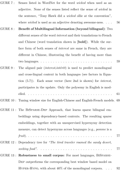
Marco saw a hairy little wampimuk crouching behind the tree.
During the winter the wampimuk hibernates in his burrow.
The girls fed their pet wampimuk berries and acorns.
Table 1: The distributional hypothesis in action: We (humans) can guess the meaning of
words likewampimuk by the context in which it appears.
How can we learn more meaningful representations for words that capture some notion of
relatedness? Intuitively, humans infer the meaning of a word from the context in which
wampimukin the sentence “Marco saw a hairy little wampimuk crouching behind the tree.”
can be guessed based on the neighboring words.1 Such patterns of word usage also allows
humans to guess that words likesquirrelorrabbitare similar towampimuk, because they can
substitute wampimuk in the above context. These observations form the basis of the field
of distributional semantics, where word meanings are modeled as a function of statistics
computed over a corpus. This intuition can be formalized in two popular distributional
semantics hypotheses.
The Distributional Hypothesis
The distributional hypothesis states that you shall know a word by the company it
keeps (Weaver, 1955; Firth, 1957; Furnas et al., 1983, inter alia). The hypothesis
has been restated differently (and more formally) over the years — words that are
similar in meaning occur in similar contexts (Rubenstein and Goodenough, 1965);
words with similar meanings will occur with similar neighbors if enough text material
is available (Schütze and Pedersen, 1995).
The definition of context and similarity in the distributional hypothesis is task-dependent.
The notion of similarity is often dictated by the representation paradigm — vector-based
word representations use a geometric similarity metric like cosine or the dot product, while
cluster-based word representations simply check for cluster overlap. Most popular
repre-sentation learning approaches define context to be the lexical neighborhood of the word
under consideration, but this choice can also be dictated by the task. For instance, in
Chapter 6, I will describe word representations that usesyntacticcontext of words to learn
representations for detecting asymmetric relations like hypernymy.
Distributed v/s Distributional. An important distinction is to be made between
dis-tributional word representations and distributed representations, A related term used in
representation learning literature (Bengio et al., 2013). Word representations that
ap-peal to the distributional hypothesis are calleddistributional representations. On the other
hand,distributedrepresentations are those where each word’s representation is described by
multiple contexts, and each context participates in describing multiple words. Distributed
representations are in contrast to local representations, such as the one-hot representation
discussed earlier. Note that a representation can be both distributional and distributed
(e.g., representations learnt using Skip-gram with Negative Sampling (SGNS), described in
Section 2.9).
While the distributional hypothesis is widely popular, it is worth noting that not all word
representation approaches appeal to it. Another related hypothesis that describes the
se-mantics of a word through statistics computed on a corpus is thebag-of-words hypothesis.
The Bag-of-Words Hypothesis
The bag-of-words hypothesis states that similar documents contain similar words,
and similar words appear in similar documents. More formally,documents that have
similar column vectors in a term-document matrix are similar (Salton et al., 1975;
Salton and Buckley, 1988).
The term-document matrix is computed by treating each document as a bag-of-words,
hence the hypothesis is referred to as the bag-of-words hypothesis. The bag-of-words
hy-pothesis examines the document level co-occurrence of words, and is close relative of the
distributional hypothesis.2 In Chapter 4, I will describe Explicit Semantic Analysis (ESA)
representations, that appeal to the bag-of-words hypothesis to represent words as the
‘bag-of-concepts’ that they describe in an encyclopedic resource like Wikipedia.
By invoking the distributional hypothesis and the bag-of-words hypothesis, representation
learning approaches can extract contextual knowledge directly from raw corpora. This
way of extracting semantics automatically is particularly appealing compared to the
time-consuming approach of hand-coding semantics (e.g., building lexical ontologies). Another
benefit of these representations is their re-usability — once extracted from a large and
2In fact, by defining the context of a word to be the documents it appears in, one can arrive at the
general enough corpora, the same word representation can be used for multiple tasks.
2.4. Cluster-based Word Representations
The problem with the one-hot representations were that they were extremely high
dimen-sional (of the size of the vocabulary), and thus did not permit any sharing. An alternative
to the crude one-hot representation is to first cluster the words in the vocabulary, such
that words that share meaningful linguistic properties gets assigned to the same cluster.
Intuitively, this cluster-based word representation reduces the effective vocabulary size to
the number of word clusters, such that words that are similar (clustered together) have
same one-hot representations. Here, I discuss one popular clustering algorithm for learning
such representations, Brown clustering (Brown et al., 1992).
The input to the Brown clustering algorithm is a corpus of wordsw1, w2,· · ·, wT, whereT
is the size of the corpus. The aim of the algorithm is to assign each word to a cluster, where
C:V →1,2,· · ·, K is a cluster assignment function that maps each word wi in the
vocab-ulary V to its clusterC(wi). The sequence of cluster assignments C(w1),C(w2),· · · ,C(wT)
for wordsw1, w2,· · · , wT is modeled using aclass-based bi-gram language model. Under this
model the generative story of the corpus is the following — transition to the current cluster
C(wi)conditioned on the previous clusterC(wi−1), sample a wordwiconditioned on the
cur-rent cluster C(wi), and repeat the process. The log-likelihood of the corpusw1, w2,· · ·, wT
(or the clustering quality) under this model is computed as,
log Pr(w1, w2,· · · , wT) = n
∑
i=1
log Pr(wi | C(wi))Pr(C(wi)|C(wi−1)) (2.2)
The output of the clustering algorithm is a binary tree, whose leaves are words, and internal
nodes are clusters of the words in the sub-tree rooted at that node. Each cluster can be
expressed using a binary code, which is the representation shared by all the words that
mutual information of adjacent clusters,
Quality(C) =∑ c,c′
Pr(c, c′)log Pr(c, c′) Pr(c)Pr(c′) −
∑
w
Pr(w)log Pr(w) (2.3)
=I(C)−H (2.4)
Thus, Brown clustering uses mutual information of adjacent clusters (i.e., at bi-gram level)
as a measure of distributional similarity between the words in those clusters. Starting with
each word in its own distinct cluster, the brown clustering algorithm greedily merges pair
of clusters that cause the smallest decrease in the likelihood of the corpus with respect to
the class-based bi-gram language model. The greedy clustering strategy naturally leads
to a hierarchical clustering upon termination. However, naively implementing this
clus-tering strategy has a run-time of O(|V|5), which was reduced to O(|V|3) in Brown et al.
(1992). Later, Liang (2005) proposed a more efficient approach that reduced the run-time
toO(|V|m2+n) by starting withm initial clusters for each of them most popular words,
wherem is number of initial clusters andnis the corpus length.
Brown clustering has proved successful in several semi-supervised scenarios, improving
per-formance on tasks like dependency parsing (Koo et al., 2008; Tratz and Hovy, 2011),
syntac-tic chunking (Turian et al., 2010), with sequence labeling tasks like named-entity recognition
enjoying large gains (Freitag, 2004; Miller et al., 2004; Ratinov and Roth, 2009).
Other Clustering Representations. Many variants of the Brown clustering algorithm
exists. For instance, Ushioda (1996) extended the Brown clustering algorithm to compute
clusters for words and phrases, while Martin et al. (1998) extended the bi-gram model
to tri-grams. Similarly, Uszkoreit and Brants (2008) used a more expressive class-based
language model that transitions to the current cluster C(wi) conditioned on the previous
clustering quality,
log Pr(w1, w2,· · · , wT) = n
∑
i=1
log Pr(wi| C(wi))Pr(C(wi)|wi−1) (2.5)
More recently, Stratos et al. (2014) noticed that the greedy strategy employed in Brown
clus-tering is simply a heuristic and is not guaranteed to recover the (provably) correct clusclus-tering
when given sufficient number of training examples. Furthermore, even with Liang (2005)’s
improved algorithm, the run-time is prohibitively long. Stratos et al. (2014) proposed an
improved cluster based representation learning approach that is guaranteed to recover the
correct clustering and runs around 10 times faster than the Liang (2005) implementation.
Limitations of Cluster-based Representations. A key limitation of using
clustering-based representations is that they are not amenable to end-to-end learning aimed at a
downstream task. This is due to the fact that the cluster assignment functionCis, in general,
discontinuous, so end-to-end learning methods like back-propagation cannot be used with
them. Furthermore, approaches like Brown clustering scale quadratically in the number
of clusters, and thus are extremely slow to train, preventing more expressive partitioning
of the space. The discreteness of the space induced by the clustering also means that the
granularity of similarity score between pair of words is discretely quantized. For instance, at
a certain level of the Brown clusters, two words either belong to the same cluster (similarity
of 1), or don’t (similarity of 0). One can circumvent this by describing a word by its path
from the root in the binary tree (e.g., apple becomes 101101). However, this approach
partially alleviates the discreteness of the space. We will see that vector space models
allow for a more expressive representation equipped with a continuous similarity measures
car bike
king queen book
magazine
muffin cake
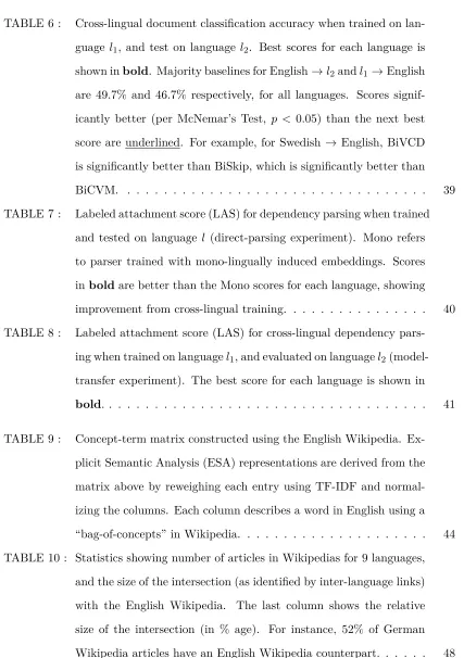
Figure 2: Vector-based word representations in a 2-dimensional space.
2.5. Vector-based Word Representations
Vector-based word representations use a point in a n-dimensional vector space to describe
each word in a language (see Figure 2). Under this representation paradigm, geometric
proximity in the vector space is used as surrogate for semantic similarity of two words. For
instance, in Figure 2, related words likeking and queen are closer than king and car. The
similarity of two wordsv and w represented in a vector space asvand wrespectively, can
then be computed using some natural geometric measure of vector proximity, like the dot
product dot(v, w) =v⊺w, or the cosine cosine(v, w) = dot|v(||v,ww|). This notion of “proximity
as a surrogate for similarity” traces its roots in cognition (Lakoff and Johnson, 1980, 1999)
as discussed in (Sahlgren, 2006).
As these representationsembed a word in a geometric space, they are also called word
em-beddings or word vectors. Over the years, several different ways of learning vector-based
word representations have been developed, that differ in the form of the vector
representa-tion (sparse or dense), and the learning framework used — count-based model and matrix
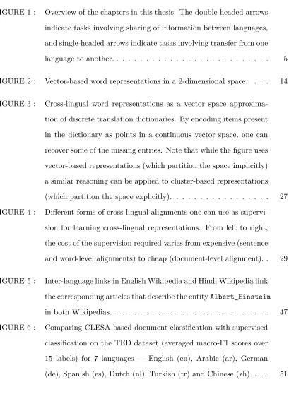
dimension→ 1st 2nd 3rd 4th 5th 6th 7th . . .
word
context
computer is of fruit breed physics bank . . .
apple 10 70 90 20 0 0 0 . . .
cat 0 60 75 5 20 0 0 . . .
interest 25 45 55 5 5 30 30 . . .
..
. ... ... ... ... ... ... ... . ..
Table 2: Example of a word-context co-occurrence matrix extracted from a corpus. Each dimension of a row corresponds to co-occurrence with a certain context word. For instance,
the word apple co-occurs with fruit (4th dimension) 20 times in the corpus.
2.6. Sparse Word Representations using Count Models
Sparse word representations (Lin, 1998a,b; Turney and Pantel, 2010; Baroni and Lenci,
2010; Levy and Goldberg, 2014a, inter alia) describe each word in the vocabulary using a
high dimensional but extremelysparse(>90% entries of the vector are 0s) vector.
The key ingredient in all sparse word representations is aco-occurrence matrixM∈R|V|×|C|,
such as the one shown in Table 2, where |V| is the size of the word vocabulary V, |C| is
the size of the context vocabulary C. The entryM[w, c]counts how often the word w∈V
has appeared in a contextc∈C.3 As a result, these approaches are also called count-based
modelsfor learning word representations (Baroni et al., 2014). The matrixM is extremely
sparse, e.g., for the text8 corpus containing about 17 million tokens and 71 thousand distinct
words, the co-occurrence matrix has ≈1% non-zero entries only (Jiang et al., 2018). The
sparsity of M is an artifact of the Zipfian distribution of words in natural language (Zipf,
1949). The representation of a word w can be directly read off the from the relevant row
w∈R|C| in the co-occurrence matrix, where|C|is the size of the context vocabulary.
Variants of count-based models differ along two dimensions — the definition of context,
and how the entries of Mare computed. As discussed in Section 2.3, the definition of the
3While I yield to the popular usage, the entries of the matrix can denote event frequencies other than
context is task-dependent, with lexical neighborhood being a popular choice. Similarly,
there are several ways to compute the entries of the co-occurrence matrixM. A naive way
of computing the entries of the occurrence matrix is to simply set each to the raw
co-occurrence frequencyn(w, c). However, raw frequency is not a good measure of relatedness
between words, because it is skewed towards co-occurrences with function words like the,
of, is etc., that do not truly reflect the semantics of the context. Different approaches of
computing the entries ofMhave been proposed to remedy this issue.
Point-wise Mutual Information (PMI). A popular approach is to weigh each entry of
the co-occurrence matrix using point-wise mutual information or PMI (Church and Hanks,
1990). PMI measures the association between word w and context c as,
P M I(w, c) =log Pr(w, c)
Pr(w)Pr(c) (2.6)
The probability of the co-occurrence is simply estimated using counts Pr(w, c) = n(w,cN ),
Pr(w) = n(Nw), Pr(c) = nN(c), wheren(w, c)is the frequency of(w, c)co-occurrence,n(w)and
n(c) are the frequencies ofw and crespectively, andN is the total corpus size. Intuitively,
PMI measures how much the probability Pr(w, c) differs from what we would expect it to
be assuming independence of Pr(w) and Pr(c) (Bouma, 2009).
Positive PMI (PPMI). An issue with PMI is that negative PMI values do not convey
meaningful information. When will PMI assume a negative value? when we have Pr(w, c)<
Pr(w)Pr(c), that is when one of w or c tend to occur individually rather than together.
For instance, this can happen when computing co-occurrences with words like the. PPMI
helps to ignore such uninformative co-occurrences. Furthermore, for unobserved(w, c)pairs
P M I(w, c) =log0 =−∞, which makes the co-occurrence matrix dense (and ill-defined).
To remedy these issues, Levy and Bullinaria (2001) suggested using positive PMI, that
Positive Local Mutual Information (PLMI). PMI and PPMI have a bias towards
rare events (i.e., smalln(w, c)). To see this, notice that for perfectly correlated wordwand
contextc (i.e., Pr(w) =Pr(c) =Pr(w, c)), the PMI or PPMI value is −log Pr(w, c), which
is higher for low Pr(w, c) (i.e., rare co-occurrences). Positive Local Mutual Information
(PLMI) (Evert, 2005, 2008) balances PPMI by including a factor for the co-occurrence
count n(w, c) of word w and context c, P LM I(w, c) = n(w, c)×P P M I(w, c). This way
rare co-occurrences get appropriately low entries inM.
Limitations of Sparse Representations. While sparse word representations do
over-come most of the limitations of one-hot word presentations, they have their own limitations.
The entries ofM are frequency estimates from a large corpus, that may be unreliable due
to chance co-occurrences of unrelated word pairs and missing evidence for unobserved but
related word pairs. Furthermore, many columns of the matrixMwill be highly correlated.
For instance, words that appear frequently with the context word big are also likely to
appear with the context wordlarge. These correlated context dimensions introduce
redun-dancy in the representation. The size of the representations also increases with the size of
the context vocabulary, just like one-hot representations.
Dense low dimensional word representations alleviate the above limitations of the sparse
word representations. These representations are dense, in that most entries in the
rep-resentation are non-zero values. Unlike sparse reprep-resentation, the reprep-resentation size is
significantly smaller than the size of the vocabulary (e.g., dense representation of size 100
can be used for a vocabulary of size 200k words). The reduced representation size also
reduces the redundancy due to correlated dimensions in the representation. Over the years,
several different approaches have been used to learn dense word representations. While
some approaches derive the dense representations by factorizing the sparse co-occurrence
matrix (eitherexactlyorapproximately), others directly learn dense representation by using