University of Pennsylvania
ScholarlyCommons
Publicly Accessible Penn Dissertations
2017
Machine Learning Methods To Identify Hidden
Phenotypes In The Electronic Health Record
Brett Kreigh Beaulieu-JonesUniversity of Pennsylvania, [email protected]
Follow this and additional works at:https://repository.upenn.edu/edissertations
Part of theBioinformatics Commons, and theGenetics Commons
This paper is posted at ScholarlyCommons.https://repository.upenn.edu/edissertations/2955 For more information, please [email protected].
Recommended Citation
Beaulieu-Jones, Brett Kreigh, "Machine Learning Methods To Identify Hidden Phenotypes In The Electronic Health Record" (2017).
Machine Learning Methods To Identify Hidden Phenotypes In The
Electronic Health Record
Abstract
The widespread adoption of Electronic Health Records (EHRs) means an unprecedented amount of patient treatment and outcome data is available to researchers. Research is a tertiary priority in the EHR, where the priorities are patient care and billing. Because of this, the data is not standardized or formatted in a manner easily adapted to machine learning approaches. Data may be missing for a large variety of reasons ranging from individual input styles to differences in clinical decision making, for example, which lab tests to issue. Few patients are annotated at a research quality, limiting sample size and presenting a moving gold standard. Patient progression over time is key to understanding many diseases but many machine learning algorithms require a snapshot, at a single time point, to create a usable vector form. In this dissertation, we develop new machine learning methods and computational workflows to extract hidden phenotypes from the Electronic Health Record (EHR). In Part 1, we use a semi-supervised deep learning approach to compensate for the low number of research quality labels present in the EHR. In Part 2, we examine and provide recommendations for characterizing and managing the large amount of missing data inherent to EHR data. In Part 3, we present an adversarial approach to generate synthetic data that closely resembles the original data while protecting subject privacy. We also introduce a workflow to enable reproducible research even when data cannot be shared. In Part 4, we introduce a novel strategy to first extract sequential data from the EHR and then demonstrate the ability to model these sequences with deep learning.
Degree Type
Dissertation
Degree Name
Doctor of Philosophy (PhD)
Graduate Group
Genomics & Computational Biology
First Advisor
Jason H. Moore
Second Advisor
Casey S. Greene
Keywords
deep learning, electronic health record, electronic phenotyping, machine learning, semi-supervised learning
Subject Categories
MACHINE LEARNING METHODS TO IDENTIFY HIDDEN PHENOTYPES IN THE ELECTRONIC
HEALTH RECORD
Brett Kreigh Beaulieu-Jones
A DISSERTATION
in
Genomics and Computational Biology
Presented to the Faculties of the University of Pennsylvania
in
Partial Fulfillment of the Requirements for the
Degree of Doctor of Philosophy
2017
Supervisor of Dissertation Co-Supervisor of Dissertation
____________________________ ____________________________
Jason H. Moore, Ph.D. Casey S. Greene, Ph. D.
Edward Rose Professor of Informatics Assistant Professor of Pharmacology
Graduate Group Chairperson
______________________
Li-San Wang, Ph.D.
Associate Professor of Pathology and Laboratory Medicine
Dissertation Committee:
John H. Holmes, Ph.D., Professor of Medical Informatics
Lyle H. Ungar, Ph.D., Professor of Computer and Information Science
MACHINE LEARNING METHODS TO IDENTIFY HIDDEN PHENOTYPES IN THE
ELECTRONIC HEALTH RECORD
COPYRIGHT
2017
Brett Kreigh Beauileu-Jones
This work is licensed under the
Dedicated to Robyn Beaulieu, Stuart Jones, William Beaulieu and Elizabeth O’Neill
ACKNOWLEDGMENTS
I would like to thank Jason Moore and Casey Greene for being incredible mentors
and advisors. I am grateful of my entire committee – John Holmes, Lyle Ungar, and
Suchi Saria for providing guidance, expertise and advice along the way. The entire
community at the University of Pennsylvania, and especially GCB created a stimulating
and encouraging environment. I would like to especially thank my cohort of GCB
students – Katie Siewart, Ian Mellis, Alex Amelie-Wolf, Lucy Shan and Salika
Dunatunga for their help adapting to Penn and preparing for the prelim. I would also like
to thank Sallie Ellison, Maureen Kirsch and Hannah Chervitz for their organizational
help and assistance transitioning to Penn.
Both the Greene and Moore labs provided ideal environments for learning and
personal development. I would like to specifically highlight Elizabeth Piette, Christian
Darabos, and Ryan Uranowicz for their support and friendship especially during the
Moore lab’s move to Penn. In the Greene lab, Jie Tan and Gregory Way provided
invaluable methods discussions and brainstorming. I would like to thank many others
from both labs for their support and feedback along the way – Jaclyn Taroni, Daniel
Himmelstein, Rene Zelaya, Kathy Chen, William LaCava, Randall Olson, Brian Cole,
Patryk Orzechowski, Alicia Cutillo, Elisabetta Manduchi, Nadia Penrod, Molly Hall and
Dan Herman.
I am grateful for all my collaborators at Penn and Geisinger Health System. Steven
Wu, Chris Bauer, and Sarah Pendergrass, especially, provided great inspiration, expertise
and were a pleasure to work with. I thank my mentee, Chris Williams, for taking on a
I would like to thank my family and friends for being an incredible support system.
My parents, Robyn and Stuart for giving me both goals and the path to achieve them. My
grandfather, William, for instilling the intellectual curiosity that has led to a love of
science. My siblings – Kyle, Megan and Brendin for challenging, teaching and
encouraging me every step of the way. My co-founders and colleagues – Alex LoVerde,
Jeff Impey, Dan Stefanis, Andrew Stephan, Chris Sullivan and Anthony Russo for
enabling me to make the transition to graduate school. Finally, Elizabeth O’Neill, for her
great support and encouragement throughout this process.
ABSTRACT
MACHINE LEARNING METHODS TO IDENTIFY HIDDEN PHENOTYPES IN
THE ELECTRONIC HEALTH RECORD
Brett Kreigh Beaulieu-Jones Jason H. Moore Casey S. Greene
The widespread adoption of Electronic Health Records (EHRs) means an
unprecedented amount of patient treatment and outcome data is available to researchers.
Research is a tertiary priority in the EHR, where the priorities are patient care and billing.
Because of this, the data is not standardized or formatted in a manner easily adapted to
machine learning approaches. Data may be missing for a large variety of reasons ranging
from individual input styles to differences in clinical decision making, for example,
which lab tests to issue. Few patients are annotated at a research quality, limiting sample
size and presenting a moving gold standard. Patient progression over time is key to
understanding many diseases but many machine learning algorithms require a snapshot,
at a single time point, to create a usable vector form. In this dissertation, we develop new
machine learning methods and computational workflows to extract hidden phenotypes
from the Electronic Health Record (EHR). In Part 1, we use a semi-supervised deep
learning approach to compensate for the low number of research quality labels present in
the EHR. In Part 2, we examine and provide recommendations for characterizing and
managing the large amount of missing data inherent to EHR data. In Part 3, we present an
adversarial approach to generate synthetic data that closely resembles the original data
research even when data cannot be shared. In Part 4, we introduce a novel strategy to first
extract sequential data from the EHR and then demonstrate the ability to model these
TABLE OF CONTENTS
ACKNOWLEDGMENTS ... iv
ABSTRACT ... vi
LIST OF TABLES ... xi
LIST OF ILLUSTRATIONS ... xii
Chapter 1. An introduction to extracting phenotypes using machine learning in the Electronic Health Record. ... 1
Motivation for using machine learning on the structured Electronic Health Record ... 1
Common Uses of Machine Learning for Structured Clinical Data ... 2
1.2.1. Patient Clustering and Disease Stratification ... 3
1.2.2. Electronic phenotypes for Genetic Associations ... 5
1.2.3. Clinical Recommendations ... 9
Challenges to Using Machine Learning on Structured Clinical Data ... 10
1.3.1. Limited research labeled “gold-standards” ... 10
1.3.2. Missing Data ... 12
1.3.3. Privacy, Reproducibility, and Data Sharing ... 16
1.3.4. Longitudinal Data ... 19
Chapter 2. Semi-‐‑Supervised Learning of the Electronic Health Record with limited “gold-‐‑standard” labels. ... 21
Abstract ... 21
Introduction ... 22
Methods ... 24
2.3.1. Unsupervised Training with Denoising Autoencoders ... 25
2.3.2. Supervised Denoising Autoencoder Classifier ... 28
2.3.3. Simulation Framework ... 28
2.3.4. Supervised Classification Comparison ... 31
2.3.5. Semi-Supervised Classification Comparison ... 32
2.3.6. Missing Data Comparison ... 32
2.3.7. Clustering and Visualization ... 33
2.3.8. ALS Survival Analysis ... 33
Results ... 34
2.4.1. Case-Control DA Training Visualization ... 34
2.4.2. Fully Supervised Comparison ... 35
2.4.3. Semi-Supervised Comparison ... 36
2.4.4. Simulated Subtype Clustering Visualization ... 39
2.4.5. ALS Survival Analysis ... 41
Summary and Future Directions. ... 42
Acknowledgements ... 45
Chapter 3. Characterizing and managing missing data in the Electronic Health Record. 46 Motivation and Introduction ... 47
Characterizing and Managing Missing Structured Data in Electronic Health Records. ... 50
3.2.1. Abstract ... 50
3.2.2. Materials and Methods ... 51
3.2.2.1. Source Code ... 51
3.2.2.2. EHR data processing ... 52
3.2.2.3. Variable selection ... 52
3.2.2.4. Predicting the presence of data ... 53
3.2.2.5. Sampling of complete cases ... 53
3.2.2.6. Simulation of missing data ... 53
3.2.2.7. Imputation of Missing Data ... 54
3.2.1. Discussion ... 63
3.2.1. Acknowledgments ... 68
Missing Data imputation in the Electronic Health Record Using Deeply Learned Autoencoders. ... 69
3.3.1. Abstract ... 69
3.3.2. ALS and the Pooled Resource Open-access Clinical Trials ... 69
3.3.3. Methods... 70
3.3.3.1. Data preparation and standardization ... 71
3.3.4. Imputation Strategies and Evaluations ... 71
3.3.4.1. Imputing missing data with Autoencoders ... 72
3.3.4.2. Comparative imputation strategies ... 74
3.3.4.3. Missing Completely at Random Imputation Evaluation ... 74
3.3.4.4. Missing Not at Random Imputation Evaluation ... 75
3.3.4.5. Progression Prediction Evaluation ... 75
3.3.5. Results ... 76
3.3.6. Missing completely at random spike-in results ... 77
3.3.7. Not missing at random spike-in results ... 78
3.3.8. ALS disease progression ... 79
3.3.9. ALS progression predictive indicators ... 80
3.3.10. Discussion and Conclusions ... 82
3.3.11. Acknowledgments ... 83
Chapter 4. Enabling data sharing and reproducible research with private data. 84 Motivation ... 84
Reproducibility of computational workflows is automated using continuous analysis. ... 85
4.2.1. Abstract ... 85
4.2.2. Introduction ... 86
4.2.3. Results ... 87
4.2.3.1. Using Docker containers improves reproducibility ... 91
4.2.3.2. Continuous Analysis ... 92
4.2.3.3. Setting up continuous analysis ... 97
4.2.3.4. Reproducible workflows ... 98
4.2.4. Discussion ... 99
4.2.5. Acknowledgements ... 101
Privacy-preserving generative deep neural networks support clinical data sharing ... 102
4.3.1. Abstract ... 102
4.3.2. Introduction ... 102
4.3.3. Results ... 105
4.3.3.1. Auxiliary Classifier GAN for SPRINT Clinical Trial Data. ... 105
4.3.3.2. Evaluation of Simulated Participants ... 107
4.3.3.3. Privacy Analysis ... 113
4.3.4. Discussion ... 114
4.3.5. Materials and Methods ... 115
4.3.5.1. SPRINT Clinical Trial Data ... 116
4.3.5.2. Auxiliary Classifier Generative Adversarial Network ... 116
4.3.5.3. Transfer Learning Task ... 117
4.3.5.4. Differential Privacy ... 117
4.3.5.5. Training AC-GANs in a Differentially Private Manner ... 118
4.3.5.6. Differentially Private Model Selection ... 119
4.3.6. Acknowledgments ... 120
Chapter 5. Taking advantage of the longitudinal aspect of Electronic Health Record data. ... 121
Abstract ... 121
Introduction ... 122
5.3.1. Source Code and Analysis Availability ... 124
Care Event Extraction ... 124
5.4.1. Medical Information Mart for Intensive Care III (MIMIC) Critical Care Database ... 124
5.4.2. Extracting Care Events from MIMIC ... 124
5.4.3. Stratification of Patient Attention based on type of Insurance Provider ... 126
Unsupervised learning to learn embeddings of extracted Care Events ... 126
5.5.1. Applying Autoencoders to Extracted Care Events to cluster in a low dimensional space. . 126
5.5.2. Predicting Survival Using Care Events ... 127
5.5.3. Traditional machine learning methods to predict survival from an EHR Snapshot. ... 127
5.5.4. Long Short Term Memory Networks (LSTMs) to predict survival with Care Events Sequences. 128 Results ... 128
5.6.1. Treatment and Outcome Comparison ... 129
5.6.2. Unsupervised modeling of patient Care Events ... 130
5.6.3. Supervised prediction of patient survival ... 131
Discussion and Conclusions ... 132
Acknowledgments ... 134
Chapter 6. Summary and Future Directions ... 135
Bibliography ... 140
LIST OF TABLES
Table 2.1 : Simulation Model 1 Parameter Sweep Specifications. ... 32 Table 2.2: Mean Receiver Operating Curve Area Under Curve by method under simulation model 1. (10
Replicate, 10-fold cross validation) ... 36 Table 3.1: LOINC codes and descriptions of the most frequently ordered clinical laboratory measurements. The assays are ranked from the most common to the least. ... 57 Table 4.1: Spearman Correlation between variable importance scores (Random Forests) and model
coefficients (Support Vector Machine and Logistic Regression). ... 113 Table 5.1: Categories and examples of Encounter Actions. ... 125 Table 5.2: Summary statistics for MIMIC Critical Care database. ... 129
LIST OF ILLUSTRATIONS
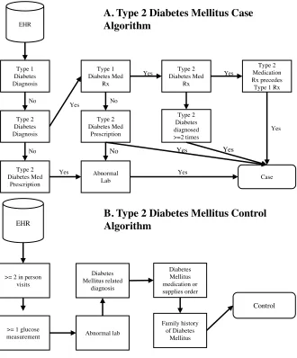
Figure 1.1: Phenotype Algorithms for Type 2 Diabetes Mellitus. ... 7
Figure 1.2: Example of case vs. control selection. ... 11
Figure 1.3: Predicting the presence of data under different missing data mechanisms. ... 13
Figure 1.4: Comparison between spike-in accuracy and variation between imputation runs. ... 15
Figure 2.1: Diagram of Denoising Autoencoder and Simulation Procedure. ... 27
Figure 2.2: Visualization of DA training over time. ... 35
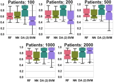
Figure 2.3: Classification AUC in relation to the number of labeled patients under simulation model 1. .... 37
Figure 2.4: Classification accuracycomparisons for models 2-4. ... 38
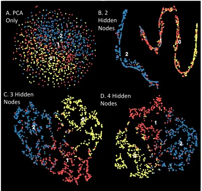
Figure 2.5: Case vs. Control clustering of 2 disease states and 1 healthy state. ... 40
Figure 2.6: Prediction comparison of ALS survival between DA constructed and raw features. ... 41
Figure 2.7: ALS Survival Visualization (Raw vs. Constructed Features). ... 42
Figure 3.1: : Mechanisms of missing data. ... 50
Figure 3.2: Summary of missing data for 143 clinical lab measures in the Geisinger Health System EHR. 56 Figure 3.3: Summary of missing data for 143 clinical lab measures in the Geisinger Health System EHR. 59 Figure 3.4: Imputation accuracy measured by RMSE across simulations 1-3. ... 60
Figure 3.5: Imputation error (RMSE) for a subset of 10,000 patients from simulation 4. ... 61
Figure 3.6: Assessment of multiple imputation for each method. ... 62
Figure 3.7 : Schematic structure of the autoencoder used for evaluations. ... 73
Figure 3.8: Imputation Evaluation Outline. ... 76
Figure 3.9: Histogram distribution and rug plot showing the number of patients each feature is present in. 77 Figure 3.10: Effect of the amount of spiked-in missing data on imputation. ... 78
Figure 3.11: Effect of non-random spiked-in missing data on imputation (measured in RMSE). ... 79
Figure 3.12: ALS Functional Rating Scale prediction accuracy. ... 80
Figure 3.13: Prediction feature importance. ... 81
Figure 4.1: Custom CDF version reporting in recent and popular publications. ... 88
Figure 4.2: Comparison of traditional vs. container based approaches. ... 90
Figure 4.3: Setting up continuous analysis. ... 93
Figure 4.4: Reproducible workflows with continuous analysis. ... 95
Figure 4.5: AC-GAN architecture and training. ... 107
Figure 4.6: Median Systolic Blood Pressure Trajectories from initial visit to 27 months. ... 109
Figure 4.7: Correlation structure between variables in the data. ... 110
Figure 4.8: Performance and Variable importance in a transfer learning task. ... 112
Figure 4.9: Privacy Parameter values during training. ... 114
Figure 5.1: Example of encounter extraction. ... 126
Figure 5.2: Association testing between different insurance types. ... 130
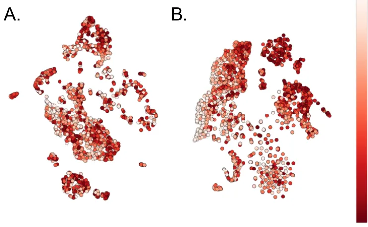
Figure 5.3: Unsupervised Encounter Embedding Visualization. ... 131
Chapter 1. An introduction to extracting phenotypes using machine learning in
the Electronic Health Record.
Portions of this chapter were adapted from: Beaulieu-Jones, Brett K. “Machine
Learning for Structured Clinical Data.” To appear in Advances in Biomedical Informatics
(Book Editors: Dawn Holmes and Lakhmi Jain), Springer. Preprint:
https://arxiv.org/abs/1707.06997
Motivation for using machine learning on the structured Electronic
Health Record
Precision medicine has the potential to substantially change the way patients are
treated in many facets of health care. Precision medicine is the idea of delivering
personalized treatment and prevention strategies by considering the holistic patient,
including their genetics, environment, and lifestyle. Machine learning using structured
clinical data will likely play a large role in the success or failure of precision medicine.
Specifically, machine learning using structure data can help in finding associations
between a patient’s genotype and phenotype, identifying similar patients and evaluating
and predicting the efficacy of different clinical treatment strategies on a personalized
level.
The amount of data collected in the clinic has rapidly expanded, the first EHRs are
now more than 20 years old and the United States federal government mandated
2015, 96% of acute care hospitals had implemented a certified EHR. Correspondingly,
several top research institutions across the country have established departments or
institutes in biomedical informatics using the EHR as a major data source in the past 5
years.
Smartphones, wearable devices and in-clinic diagnostic tools offer the ability to
stream accurate measurements in real time. AliveCor received FDA approval in 2012 for
its iPhone-based heart monitor using machine learning to detect Atrial Fibrillation in
seconds. Billions of dollars in venture capital are currently being invested in companies,
such as Grail, Foundation Medicine, and Guardant health, promising less invasive
biopsies, or liquid biopsies, using machine learning to classify patients from circulating
tumor cells in the bloodstream. Preventative wellness clinics, such as Forward, are
emerging to characterize and track what it means to be healthy.
These are only a few examples of the many opportunities centered on patient data.
Data for both evidence-based clinical decision making and computational research is
becoming increasingly available and we must now develop new methods to preprocess
and analyze this data at a matching rate.
Common Uses of Machine Learning for Structured Clinical Data
Each time a patient interacts with a health system, actions, notes, and measurements
are recorded in the EHR. This wealth of data has made the EHR the primary source of
structure clinical data. Three promising research applications of EHR data are:
1.) Patient clustering and disease stratification.
2.) Electronic phenotyping for genetic studies.
These tasks can be performed using machine learning, but each task requires careful
preprocessing of data and appropriate phrasing of the problem to utilize traditional
machine learning methods. The nature of EHR data places emphasis on unsupervised
clustering and semi-supervised classification. In this section, we discuss these common
tasks and show examples where researchers have utilized machine learning effectively to
guide discovery. There exist many great resources for understanding machine learning
approaches as applied to general problems (1). We concentrate on how to position
relevant clinical questions and the challenges specific to the EHR that need to be solved
in order to apply these powerful techniques.
1.2.1. Patient Clustering and Disease Stratification
As we learn more about the mechanisms and etiology of a disease, our diagnoses can
become more precise, leading to the creation of disease subtypes. Historically, cancers
were diagnosed based on their occurrence location and their reaction to different
treatments. As the mechanisms of cancer are better understood, they are further
categorized by their physiological nature. The progression of subtypes in lung cancer
illustrates the increases in resolution over time for a previously poorly defined disease
(2). Beginning with a single diagnosis based on occurrence in the lung, it was later
differentiated as small cell lung cancer and non-small cell lung cancer (3, 4). Non-small
cell lung cancer was then broken up into squamous cell carcinoma, adenocarcinoma, and
large cell carcinoma. Today these subtypes continue to be broken up based on the genetic
locations and pathways of associated risk variants.
What happens when physiological differences cannot easily be used to subtype
has been redefined numerous times. It is associated with a wide range of comorbidities
and presents in a clinically heterogeneous manner. These comorbidities, including
coronary heart disease, diabetes, and stroke, represent an oversized risk to public health
and increasingly unwieldy burden on the health care system. Despite this, metabolic
syndrome’s predictive value for cardiovascular events, disease prediction and progression
is disputed and may not outperform the individual components that define it (5). While
the concept of identifying patients at high risk of developing diseases such as heart
disease and diabetes for early intervention is an important one, metabolic syndrome in its
current form fails to do this effectively.
Li et al. demonstrated the ability to identify disease subtypes of patients with a
metabolic disorder, type 2 diabetes (6). To do this they performed a topological analysis
of 11,210 patients with type 2 diabetes at Mount Sinai Medical Center in New York. This
topological analysis constructed a network of patients by connecting those most similar to
each other. Using this they found three unique subtypes. Subtype 1 demonstrated the
traditional observations of type 2 diabetes, hyperglycemia, obesity, and eye and kidney
diseases. Subtype 2’s main comorbidity was cancer, and subtype 3’s unique
comorbidities were neurological diseases. These subtypes are likely enriched for
etiological differences; the disease likely operates differently in someone who develops
cancer than someone who develops kidney disease. By developing a machine learning
classifier to identify which subtype a patient is in as early as possible, clinicians may be
able personalize treatment to reduce the odds of developing these more serious
Multiple sclerosis illustrates an area machine learning for disease stratification could
be particularly useful. Multiple sclerosis was traditionally subtyped into
Relapsing-Remitting MS and Progressive MS. In 2014, it was recommended that these subtypes be
further divided into six total subtypes (7). Unfortunately, the current strategies for
determining subtype and thus treatment strategy require looking at the progression of the
disease. This is essentially a retrospective diagnosis and means personalized treatment
plans cannot be started until progression has been observed. Could unsupervised
clustering be used to identify subtypes earlier on?
1.2.2. Electronic phenotypes for Genetic Associations
Genetic associations examine whether a genetic variant is associated with a specific
trait. This specific trait, a phenotype, can be a moving target when dealing with the
complexity of human disease. The trait is often a human defined disease. Those with the
disease are labeled the case and those without the disease are considered controls. Early
genetic associations using the electronic health record were performed with raw
International Classification of Diseases (ICD) codes. ICD codes are recorded by
physicians when diagnosing a patient with a condition, and are used to ensure proper
billing and insurance reimbursement. ICD codes are published and updated by the World
Health Organization and are primarily used for clinical billing purposes. Despite ICD-10
being initially published in 1994, ICD-9 codes are still commonly used in both clinical
and research settings.
While ICD codes provide a clear, discrete endpoint for genetic associations, the use
of billing codes can introduce unintentional biases to analyses. An ICD code may be
screen for the disease the ICD code represents. In this case, not only is the timing of
diagnosis difficult to determine, but solely looking at the ICD codes for a patient is likely
to introduce false positives. In addition, certain ICD codes are more easily reimbursed
than others. When a clinician determines that a patient requires a treatment or test to
increase their odds of a successful outcome, the clinician is incentivized to choose the
ICD code most likely to allow them to effectively treat their patient.
Phenotype algorithms can be developed using the structured EHR to leverage both
ICD codes and the rest of the of a patient’s record. The eMERGE project is a national
network which has deployed phenotype algorithms for over 40 diseases, over 500,000
EHRs and 55,000 patients with genetic data. Many of the phenotype algorithms are
Figure 1.1: Phenotype Algorithms for Type 2 Diabetes Mellitus.
A.) Case selection from the EHR. B.) Control Selection from the EHR. Adapted from: (8).
An approach to study phenotype-genotype associations from the EHR are
Phenome-wide association studies or PheWAS (8). PheWAS use EHRs to define a phenome that
can be linked back to individual genetic variants. The approach can discover gene-disease
associations while identifying pleiotropic effects of individual SNPs. PheWAS generally
uses the ICD9 codes to construct a phenotype. While primarily used for billing, these
codes provide a set of discrete variables that can represent many phenotypes for a patient
at the same time, providing greater resolution. Besides the repurposing of billing codes, a
Type 1 Diabetes Diagnosis Type 2 Diabetes Diagnosis Type 1 Diabetes Med Rx Type 2 Diabetes Med Prescription Abnormal Lab No EHR Yes Case Type 2 Diabetes Med Rx Type 2 Diabetes diagnosed >=2 times Type 2 Medication Rx precedes Type 1 Rx
Type 2 Diabetes Med Prescription Yes No Yes Yes Yes Yes No Yes No Yes
A. Type 2 Diabetes Mellitus Case Algorithm
B. Type 2 Diabetes Mellitus Control Algorithm
>= 2 in person visits EHR
>= 1 glucose
major challenge of PheWAS is in understanding the functional mechanisms at work
behind GWAS SNP matches. Stratification by the 4,841 different codes creates wide
data, presenting statistical challenges in achieving adequate power. This challenge of
achieving adequate power will be exacerbated by the transition to ICD10, with less
historical data built up and the potential for over 16,000 codes. Continuing to increase
open data access will allow researchers to utilize a more accurate phenotypic
representation while lessening the burden of statistical challenges. Coding systems,
unlike patient notes or genomic data should be easier to anonymize, aggregate, and
distribute.
ICD billing codes can be biased, as evidenced by phenotype algorithms having
multiple steps to catch errors for both case and control status, using billing codes alone
may cause misclassification of phenotypes. The misclassification of phenotypes
substantially reduces the power to detect linkage in case-control studies. With 1%
phenotypic misclassification up to 10% of the power is lost, and with 5% phenotypic
misclassification, the power is reduced by approximately two-thirds (9–11).
Misclassification can occur for a variety of reasons including misdiagnosis/clinical error,
clerical error, or lack of scientific knowledge about the disease in question.
Labbe et al. showed increased linkage by clustering lifetime symptoms in
schizophrenia and bipolar disease to form more homogenous phenotypes. Separating
cases by the symptoms of psychiatric diseases compensates for the inability to subtype
these diseases by physical properties (12). This is important due to the deficit of
physiological understanding for these diseases. Labbe et al. also included familial
that show a strong familial aggregation they observed higher linkage scores. By looking
at ancestral histories for subtypes, the expected heritability could be better estimated
resulting in a reduction of “missing heritability.”
Phenotypic subtyping was also used successfully in the analysis of genetic variants
responsible for the severe development regression and stereotypical hand movements of
Rett syndrome. Causal mutations were found in the FOXG1 and MECP2 genes and
deletions at the 22q11.2 locus (13).
Each of these examples point towards the promise of using machine learning to
cluster patients based on their EHRs to identify disease subtypes or more homogenous
groups of patients for use in association studies.
1.2.3. Clinical Recommendations
The availability of data and advances in biomedical informatics have helped to make
medicine increasingly evidence based and in some cases entirely data driven. Clinicians
and researchers now have the ability to leverage millions of data points when designing
and determining treatment best practices. The New England Journal of Medicine recently
held the SPRINT data analysis to “use the data underlying a recent article to identify a
novel clinical finding that advances medical science.” The original clinical trial sought to
see whether intensive management of systolic blood pressure (<120 mm Hg) was more
effective than standard management (<140 mm Hg). The original trial was stopped early
due to the success of the intensive management strategy in reducing cardiovascular
events. The data from the trial was released as a challenge where teams used machine
More personalized treatment strategies are a popular use of machine learning in the
EHR. This can be driven by genomics (pharmacogenomics), or simply by sub setting
patients based of attributes (race, BMI, etc.). Wiley et al. demonstrate the importance of
training an algorithm on a population similar to the application population (14). In their
case it was necessary to extract the percent African ancestry from the genome instead of
self reported race in order to improve the model fit.
Due to the inherent risk of adjusting clinical treatment strategies, many of the early
applications of machine learning in health systems have been seen in academic research
(retrospective analysis, drug development, pharmacogenomics) and for things like
resource usage. For example, how likely is a patient coming into the ER to need an ICU
bed? Increasingly machine learning methods are likely to be applied to clinical decisions
including providing prognosis information for shared decision making strategies. Deep
learning, in particular, is becoming an increasingly tool for drug discovery and
development (15).
Challenges to Using Machine Learning on Structured Clinical Data
1.3.1. Limited research labeled “gold-standards”
Large institutions and health care systems can have EHRs containing millions of
patients and billions of measurements. Despite the size of these data, electronic
phenotyping requires a gold standard to validate accuracy. This gold standard often
requires time consuming, manual clinician review and is thus expensive.
In addition, the selection of cases and controls can unintentionally create biases in
and the healthiest controls. In these circumstances researchers can have the greatest
confidence they are accurately selecting a true case or control. Unfortunately, this creates
a biased training set where it is difficult to differentiate between less severe cases and less
healthy controls. Figure 1.2 shows an illustration of a simulated dataset where the first
two principal components happen to represent the degree of the case phenotype. If the
most severe cases are selected, a classifier trained to distinguish between cases and
controls is unlikely to generalize well. If less severe cases are chosen, there may be issues
with mislabeled cases.
Figure 1.2: Example of case vs. control selection.
Simulated disease severity plot where the 2 principal components stratify patients according to severity.
An example of another bias can be seen in the Type 2 Diabetes Mellitus algorithm,
controls must have at least 1 glucose measurement (Figure 1.1 B). For a young patient,
this means that a clinician must have had reason to suspect that the patient’s glucose
could be abnormal and thus could bias controls to patients who “look” like they are at a
high risk for developing Type 2 Diabetes.
Because patients move between health systems, a patient may not be diagnosed in
the system they are treated in and may only have a partial history. Some methods for
controlling for incomplete histories can result in smaller sample sizes. It is common to
include only patients who have a visit in the system prior to the diagnosis of the
phenotype of interest. While this can help to determine the diagnosis date for a disease, it
excludes anyone who was diagnosed on their first visit to a particular health system.
1.3.2. Missing Data
The average patient is unlikely to have measurements for the clear majority of fields
in the EHR. It does not make sense logistically or economically to administer every test
to a seemingly healthy patient. There are three primary types of missing data:
1.) Missing Completely at Random (MCAR) – when data is missing in a completely unrelated way to the values of both the observed and the unobserved data.
2.) Missing at Random (MAR) – when the data is missing based on the observed data, when other fields in the EHR indicate whether the value will be present or absent.
3.) Missing Not at Random (MNAR) – when the data is missing based on the values of the unobserved data.
be predicted (Figure 1.3 A), and data that is either MAR or MNAR (Figure 1.3 B, 1.3 C)
can be predicted with an accuracy significantly greater than random. In practice, most
missing data in the EHR tends to be of the MAR variety. Clinicians must decide which
measurements are relevant and fiscally responsible, irrelevant tests are wasteful and it
does not make sense to subject patients to unnecessary discomfort. The clinician is
making these decisions based on the observations they make, so when data is missing it is
related to the observed data.
Figure 1.3: Predicting the presence of data under different missing data mechanisms.
A.) Data that is missing completely at random cannot be predicted. B & C.) Data that is missing at random and missing not at random can be predicted at better than random accuracy (to appear
(16)).
MCAR data is less likely to present issues to downstream analyses than data that is
introduce unintentional biases to all sorts of downstream analyses including machine
learning. Machine learning algorithms often expect a complete matrix as input and are
not designed to handle null values. This often leads to researchers performing one of
three options:
1.) Perform feature selection of relevant features and use only complete cases, or patients that have values for all features.
2.) Modify the algorithm to accept null inputs (often by ignoring them) or
3.) Perform imputation to predict what the value for a feature would be.
Each of these options have several pros and cons and can have unintended effects on
machine learning. When performing complete case analysis after feature selection, the
features included can lead to including either more severe cases or cases that were harder
to diagnose. Imagine a disease that is diagnosed by a laboratory measurement where
values over 10 conclusively indicate you have the disease but values between 8 and 10
require an additional test. If the additional test is included in the features selected, the
complete cases are now only the patients that were harder to diagnose. When modifying
an algorithm to accept null inputs, the researcher needs to be careful that the algorithm
does not disproportionately learn to depend on patients that have all of the measurements
or only the most complete measurements. If the algorithm relies on patients with all of
the measurements, many of the same issues that arise in complete case analysis repeat. If
the algorithm learns to ignore rare measurements it can miss signal. For example, in an
analysis of different treatment options, say 40 of 10,000 patients suffered a fairly rare but
severe adverse event. Without careful monitoring the algorithm may not place enough
Figure 1.4: Comparison between spike-in accuracy and variation between imputation runs.
Imputation can be effective in the EHR because many missing values can be inferred
by omission and just knowing whether a value was present or absent can be useful. If a
patient has never had a chest x-ray, it is unlikely that their physician suspects a broken rib
cage. This information can be provided to downstream machine learning algorithms by
performing imputation. It is, however, very important to carefully analyze the results of
imputation. Oftentimes much can be learned simply by looking at which methods are the
most accurate. Direct accuracy can be measured by spiking in missing values to replace
known values, imputing these spiked-in values and measuring their difference from the
real values. Despite this direct accuracy should only be used as a benchmark, and it is
important to analyze the effect of imputation on the downstream analyses you are
performing (Figure 1.4).
For example, mean imputation may perform strongly in an analysis using spiked-in
missingness but remove all variance from the imputed values for a feature (Figure 1.4 C).
Other evaluation criteria, such as, comparing the variance between imputed values of
different imputation runs and the difference between imputed values and real values.
Ideally these values would be highly correlated in order to maintain the variance
RMSE Imputed vs. Spike-in RMSE Imputed vs. Spike-in RMSE Imputed vs. Spike-in
D if fe re nc e be tw ee n im put at ion r uns D if fe re nc e be tw ee n im put at ion r uns D if fe re nc e be tw ee n im put at ion r uns
structure. Popular imputation methods for EHRs include K-Nearest Neighbors, Singular
Value Decomposition and Multiple Imputation by Chained Equations.
All three of these strategies for handling missing data may introduce bias when
performing EHR-based analyses. It is important to consider potential effects and ideally
to utilize multiple strategies and examine the differences.
1.3.3. Privacy, Reproducibility, and Data Sharing
Patient privacy needs to be a focus of any secondary use of EHRs. Because a patients
EHR is ‘de-identified’ does not mean that it is anonymous. Latanya Sweeney
demonstrated this emphatically when the Massachusetts Group Insurance Commission
released de-identified data on state employees (17). These records included each hospital
visit and Sweeney re-identified several patients including the former Governor of
Massachusetts. Sweeney did this from his birth date, zip code and sex alone, and to prove
a point mailed the Governor a copy of his personal records. The task of re-identification
has been shown possible in several other cases where data holders attempted to share
their data, including the Netflix challenge. Narayana and Shmatikov were able to
de-anonymize users in the Netflix challenge by linking their viewing histories with popular
movie review sites. For users who had rated more than 6 movies, they were able to do
this with greater than 90% accuracy (18). This, in part, led to Netflix canceling the
second iteration of its popular recommendation contest following a privacy lawsuit.
Caution needs to be taken even when the actual data is not released. Deep learning
models can have many millions of parameters, allowing adversaries to perform
membership inference attacks in order to determine whether a user was a member of the
examples in the training set. They do this by examining the trained parameters of a deep
neural network trained on the CIFAR-100 dataset. Even without the model, enterprising
adversaries performed membership inference attacks with only black-box access to the
target model through an API. Shokri et al. again demonstrated this on various purchase
history datasets made available through Amazon and Google APIs.
One approach to adding privacy protection is called “Differential Privacy” (20).
Differential Privacy is a robust, meaningful and mathematical rigorous definition of
privacy which operates under the knowledge that data cannot be fully anonymized and
remain useful. If you remove all of the signal in a dataset to anonymize, machine learning
methods are fruitless. If you keep any signal at all, there is a chance an adversary will
able to discover information about the members of the dataset. The goal of differential
privacy is to find a balance between an acceptable risk, the privacy budget, and
usefulness of the data. It attempts to minimize the likelihood an adversary can perform a
membership inference attack to determine if a subject is in a dataset. It works by adding a
plausible deniability of any outcome by inserting random noise into the information made
available. If balanced, meaningful answers can be interrogated from the data while
greatly reducing the risk that any member of a study is harmed by de-identification. A
classic example and simple way to think about differential privacy is to imagine a study
where participants are told to answer a question. Before answering the question they flip
a coin, if the coin lands heads, they give the real answer, the truth. If the coin lands tails,
they answer randomly by flipping an additional coin and responding yes if it lands heads
Simmons et al. used a variant of differential privacy to enable privacy preserving
genome wide association studies even when there is significant population stratification.
Genomic data has a high dimensionality and relatively low signal to noise ratio making
de-identification or other attempts at masking individual records impractical. They
demonstrate the ability to allow users to query summary statistics while minimizing
privacy risks. This is a particularly interesting application because while genome
sequencing prices have rapidly decreased, the combined costs of recruitment and
sequencing are a major barrier to this type of research. This method allows for increased
sharing of valuable, difficult to obtain datasets. Differential privacy is a rapidly growing
area, we suggest “The Algorithmic Foundations of Differential Privacy” (21) as a starting
point if interested in implementing differential privacy.
Privacy challenges can make sharing data prohibitively difficult. This in turn
presents challenges in reproducing work from other researchers. Even if source code is
shared, researchers attempting to reproduce original research generally can only compare
final results. This means that even if a protocol of a paper is well written and described, if
it has 100 steps, a researcher attempting to reproduce cannot be sure where their results
diverged. Because of this challenge we strongly advocate publishing intermediate results.
This can help narrow down divergences to a few steps, was it the data? The
preprocessing? The actual analysis? The plotting into charts? One way to release
intermediate results without adding a large amount of additional work is to use
1.3.4. Longitudinal Data
A key attribute and potential strength of EHRs is the ability to track the way a patient
progresses over time. Early moving caregivers such as Geisinger Health System
implemented initial EHRs over twenty years ago but fully utilizing this longitudinal
presents challenges to researchers.
Longitudinal EHR data are often irregular time series. Measurements are recorded at
irregular times, can be mixed type (continuous, ordinal, categorical), require feature
extraction (images, free text). It is common for researchers to take a single time point (i.e.
current time, set time after diagnosis etc.) and use this as the single end point or label for
machine learning analyses. This can be problematic when patients have arrived at that
point through very different routes. For example, if using a systolic blood pressure as an
end point, one patient may be on an intensive blood pressure management protocol while
another with the same blood pressure may have never taken medication. In the SPRINT
clinical trial there were patients on as many as seven medications to manage blood
pressure (23), if unmedicated these patients would almost definitely have significantly
higher measurements. One method researchers use to remediate this issue is to derive
statistics to represent the time series, such as taking the median value. This can be
insufficient when the way clinicians choose to observe and treat patients based on data
either not recorded in the electronic health record, in the unstructured data or in fields not
selected for inclusion can also bias the labels. For example, if patient A has a single
normal white blood cell count, and patient B has had a monthly count every month for
the past 5 years. A clinician could have been checking to see if patient A showed an
contrast, the repeated measurements for patient B indicate the clinician may have a
reason to believe patient B is immunocompromised or may become
immunocompromised due to a virus or adverse reaction to a medication and is using the
white blood cell count to monitor this. Despite the patients having relatively equal white
blood cell counts, using this single value as a label is clearly inadequate to represent the
complete state of the patient. For this specific case deriving a panel of statistics including
features such as the count and variance of the measurement could help to better represent
the current state of a patient. Recent work takes this further to calculate disease and
patient trajectories by generating networks of the way a patient or disease progresses over
time. Jensen et al. demonstrated this using 6.2 million patients from Danish National
Patient Registry to cluster patients based on time dependent disease diagnoses (24).
These disease diagnoses were extracted from patterns of ICD-9 codes on patient’s EHRs.
This method creates a visualization of patient trajectories and allows for analyses of
co-morbidities observed in health systems in order to identify important patterns that
indicate the potential for more severe outcomes. Further work in this field could move
Chapter 2. Semi-Supervised Learning of the Electronic Health Record with
limited “gold-standard” labels.
This chapter was originally published as: Beaulieu-Jones, Brett K., Casey S. Greene, and
the Pooled Resource Open-Access ALS Clinical Trials Consortium. "Semi-supervised
learning of the electronic health record for phenotype stratification." Journal of
biomedical informatics 64 (2016): 168-178. doi: 10.1016/j.jbi.2016.10.007
B.K.B.-J. and C.S.G. conceived the study and designed the solution. B.K.B.-J.
implemented and performed the analysis. B.K.B.-J. and C.S.G. wrote, revised and
approved the manuscript.
Data used in the preparation of this article were obtained from the Pooled Resource Open-Access ALS Clinical Trials (PRO-ACT) Database. As such, the following organizations and individuals within the PRO-ACT Consortium contributed to the design and implementation of the PRO-ACT Database and/or provided data, but did not participate in the analysis of the data or the writing of this report: Neurological Clinical Research Institute, MGH, Northeast ALS Consortium, Novartis, Prize4Life, Regeneron
Pharmaceuticals, Inc., Sanofi, Teva Pharmaceutical Industries, Ltd.
Abstract
Patient interactions with health care providers result in entries to electronic health
records (EHRs). EHRs were built for clinical and billing purposes but contain many data
points about an individual. Mining these records provides opportunities to extract
electronic phenotypes, which can be paired with genetic data to identify genes underlying
common human diseases. This task remains challenging: high quality phenotyping is
costly and requires physician review; many fields in the records are sparsely filled; and
evaluate a semi-supervised learning method for EHR phenotype extraction using
denoising autoencoders for phenotype stratification. By combining denoising
autoencoders with random forests we find classification improvements across multiple
simulation models and improved survival prediction in ALS clinical trial data. This is
particularly evident in cases where only a small number of patients have high quality
phenotypes, a common scenario in EHR-based research. Denoising autoencoders perform
dimensionality reduction enabling visualization and clustering for the discovery of new
subtypes of disease. This method represents a promising approach to clarify disease
subtypes and improve genotype-phenotype association studies that leverage EHRs.
Introduction
Biomedical research often considers diseases as fixed phenotypes, but many have
evolving definitions and are difficult to classify. The electronic health record (EHR) is a
popular source for electronic phenotyping to augment traditional genetic association
studies, but there is a relative scarcity of research quality annotated patients (25).
Electronic phenotyping relies on either codes designed for billing or time intensive
manual clinician review. This is an ideal environment for semi-supervised algorithms,
performing unsupervised learning on many patients followed by supervised learning on a
smaller, annotated, subset. Denoising autoencoders (DAs) are a powerful tool to perform
unsupervised learning (26). DAs are a type of artificial neural network trained to
reconstruct an original input from an intentionally corrupted input. Through this training
they learn higher-level representations modeling the structure of the underlying data. We
annotated patients required, construct non-billing code based phenotypes and elucidate
disease subtypes for fine-tuned genetic association.
The United States federal government mandated meaningful use of EHRs by 2014 to
improve patient care quality, secure and communicate patient information, and clarify
patient billing (27, 28). Despite not being designed specifically for research, EHRs have
already proven an effective source of phenotypes in genetic association studies (29, 30).
Initially, phenotypes were hand designed based on manual clinician review of patient
records. These studies were limited by the time and cost inherent in manual review (31,
32), but DAs can make use of unlabeled data. After unsupervised pre-training, the trained
DA’s hidden layer can be used as input to a traditional classifier to create a
semi-supervised learner. This allows the DA to learn from all samples, even those without
labels, and requires only a small subset to be annotated. Today, phenome-wide
association studies (PheWAS) are the most prevalent example of EHR phenotyping,
proving particularly effective at identifying pleiotropic genetic variants (33). PheWASs
often use algorithms based on the International Classification of Disease (ICD) codes to
construct a phenotype. This coding system was designed for billing, not to capture
research phenotypes. DA constructed features are combinations of many components of
clinical data and may provide a more holistic view of a patient than billing codes alone.
Through extensive study, disease diagnoses can become more precise over time (2–
4, 34, 35). Cancers, for example, were historically typed by occurrence location and the
efficacy of different treatments. As the mechanisms of cancer are better understood, they
are further categorized by their physiological nature. The progression of subtypes in lung
diagnosis based on occurrence in the lung, lung cancer has been divided into dozens of
subtypes over several decades based on histological analysis, and genetic markers (2–4,
35). The unsupervised nature of DAs means that even if the definitions of a disease
change, they would not need to be retrained. The ability to identify more homogenous
phenotypes showed increased genotype to phenotype linkage in schizophrenia, bipolar
disease (12), and Rett Syndrome (13, 36–38). Furthermore, type 2 diabetes subtypes have
been discovered using topological analysis of EHR patient similarity (6). The
dimensionality reduction possible with a DA makes clustering and visualization more
feasible. Subtyping exposes disease heterogeneity and may contribute to additional
physiological understanding.
Previous work in semi-supervised learning of the EHR relies on closed source
commercial software (6), and natural language processing of free text fields to match
clinical diagnosis (39, 40). We are not aware of any previous work performing
semi-supervised classification and clustering from quantitative structured patient data.
Methods
We developed an approach, entitled “Denoising Autoencoders for Phenotype
Stratification (DAPS),” that constructs phenotypes through unsupervised learning. This
generalized phenotype construction can be used to classify whether patients have a
particular disease or to search for disease subtypes in patient populations. To evaluate
DAPS, we created a simulation framework with multiple hidden factors influencing
potentially overlapping observed variables. We evaluated the reduced DA models against
feature-complete representations with popular supervised learning algorithms. These
incompletely labeled and missing data. We developed a technique that uses the reduced
feature-space of the DA to visualize potential subtypes. Finally, we evaluate DAs ability
to predict ALS patient survival in both classification and clustering tasks. Each of these is
fully described below and full parameters included in sweeps are available in the
supplementary materials.
Source code to reproduce each analysis is included in our repository
(https://github.com/greenelab/DAPS) (41) and is provided under a permissive open
source license (3-clause BSD). A docker build is included with the repository to provide
a common environment to easily reproduce results without installing dependencies (42).
In addition, Shippable, a continuous integration platform, is used to reanalyze results in a
clean environment and generate figures after each commit (43).
2.3.1. Unsupervised Training with Denoising Autoencoders
DAs were initially introduced as a component in constructing the deep networks
used in deep learning (44). Deep learning algorithms have become the dominant
performers in many domains including image recognition, speech recognition and natural
language processing (45–50). Recently they have also been used to solve biological
problems including tumor classification, predicting chromatin structure and protein
binding (26, 51, 52). DAs showed strong performance early in the deep learning
revolution but have been surpassed in most domains by convolutional neural networks or
recurrent neural networks (44). While these complex deep networks have surpassed the
performance of DAs in these areas, they rely on strictly structured relationships such as
the relative positions of pixels within an image (47, 53). This structure is unlikely to exist
are easily generalizable, benefit from both linear and nonlinear correlation structure in the
data, and contain accessible, interpretable, internal nodes (26). Oftentimes the hidden
layer is a “bottle-neck”, a much smaller size than the input layer, in order to force the
autoencoder to learn the most important patterns in the data (53).
We used the Theano library (54, 55) to construct a DA consisting of three layers, an
input layer x, a single hidden layer y, and a reconstructed layer z(44) (Figure 2.1A).
Noise was added to the input layer through a stochastic corruption process, which masks
20% of the input values, selected at random, to zero.
The hidden layer y was calculated by multiplying the input layer by a weight vector
W, adding a bias vector band computing the sigmoid (Formula 1). The reconstructed
layer z was similarly computed using tied weights, the transpose of W and b (Formula 2).
The cost function is the cross-entropy of the reconstruction, a measure of distance
between the reconstructed layer and the input layer (Formula 3).
𝑦 = 𝑠 𝑊𝑥 + 𝑏 (Formula 1)
𝑧 = 𝑠 𝑊)𝑦 + 𝑏) (Formula 2)
𝑐𝑜𝑠𝑡 = − 4 [𝑥0log 𝑧0
056 + (1 − 𝑥0) log 1 − 𝑧0 ] (Formula 3)
Stochastic gradient descent was performed for 1000 training epochs, at a learning
rate of 0.1. Hidden layers of two, four, eight and sixteen hidden nodes were included in
the parameter sweep with a 20% input corruption level. Vincent et al. (44) provide a
through explanation of training for DAs without missing data.
In the event of missing data, the cost calculation was modified to exclude missing
data from contributing to the reconstruction cost. A missingness vector m was created for
missing. Both the input sample x and reconstruction z were multiplied by m and the
cross-entropy error was divided by the sum of the m, the number of non-missing features to get
the average cost per feature present (Formula 4). This allowed the DA to learn the
structure of the data from present features rather than imputation.
𝑐𝑜𝑠𝑡 = − 4056[𝑥0log 𝑧0 𝑚0+ (1 − 𝑥0) log 1 − 𝑧0 𝑚0] / 𝑐𝑜𝑢𝑛𝑡(𝑚)
(Formula 4)
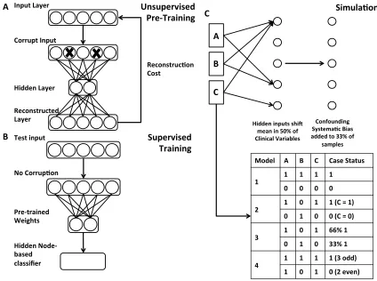
Figure 2.1: Diagram of Denoising Autoencoder and Simulation Procedure.
A.) Network diagram of DAs used for unsupervised pre-training. Input data is intentionally corrupted and then weights and biases are learned to minimize reconstruction cost when mapping the data to a hidden layer and back to a reconstructed layer. B.) Supervised classification occurs using the pre-trained DA hidden nodes as input to a traditional classifier. C.) Simulation model with example cases and controls under each rule set.
Unsupervised Pre-Training
Hidden inputs shi4 mean in 50% of Clinical Variables
Confounding SystemaBc Bias added to 33% of
samples
A
B
C
Model A B C Case Status
1 1 1 1 1
0 0 0 0
2 1 0 1 1 (C = 1)
0 1 0 0 (C = 0)
3 1 0 1 66% 1
0 1 0 33% 1
4 1 1 1 1 (3 odd)
1 0 1 0 (2 even)
2.3.2. Supervised Denoising Autoencoder Classifier
To convert the DA to a supervised classifier, we first trained the DA in an
unsupervised fashion (pre-training) (Fig 2.1 A). We then applied a variety of traditional
machine learning classifiers including, decision trees, random forests, logistic regression,
nearest neighbors and support vector machines to the pre-trained unsupervised hidden
layer values, y, of the DA (Figure 2.1 B). Random forests applied to DA hidden nodes
(DA+RF) were shown for all comparisons. Predictive performance was measured by
comparing the AUROC using stratified 10-fold cross validation. The Scikit-learn library
was used for the traditional classifiers (56). The Support Vector Machine uses a radial
basis function kernel, with a penalty parameter of 1. The nearest neighbors classifier uses
a k-value of 5 and the random forest uses 10 estimators. These parameters achieved
optimal performance in a preliminary parameter sweep.
2.3.3. Simulation Framework
We designed four simulation models to evaluate algorithmic performance. These
simulations were not designed to perfectly recapitulate EHR data. Instead they are
designed to capture a variety of complexity in order to identify algorithmic strengths and
weaknesses with known underlying models.
To simulate patients, first clinical observations were generated by first drawing
random samples from a normal distribution. Next hidden input effects were generated in
accordance with one of four simulation models. When turned on these hidden input
effects shift 1 to N observed clinical variables with replacement (Figure 2.1 C). Shifted
clinical features were chosen at random, but consistent for all patients. Case-control
effect being on and 0 represents the effect being off. Next, a confounding systematic bias
was added to a random subset (33%) of the patients as a source of additional noise to
simulate the variance accompanying data created by physicians, labs, hospitals or other
spurious effects.
There are four models defining hidden input effect rules to determine case-control
status:
1. All together/all relevant. Individuals have the same value (0 or 1) for all hidden input effects. Controls have all hidden effects set to 0. Cases have all hidden effects set to 1. A model capturing any hidden input will be able to predict case/control status in this scenario. This is a test of whether each method can recognize any of the hidden effects.
2. All independent /single effect relevant. Individuals have 0 to N (specified per simulation) hidden input effects chosen at random. One arbitrary effect (the last one) is used to determine case-control status. In controls, this is 0. In cases, this is 1. A model capturing the relevant hidden input will be able to predict
case/control status in this scenario. This is a test of whether each method can recognize the important hidden effect when there are multiple shifted
distributions.
3. All independent/percentage based. Individuals have 0 to N (specified per simulation) of hidden input effects chosen at random set to 1. The percentage of hidden input effects on represents the probability of the patient being a case. A model capturing more hidden effects will be able to more accurately predict case/control in this scenario. This is a test of whether each method can perform effectively without a hard-rule based model, and could represent a disease with incomplete penetrance.