Patron: Her Majesty The Queen Rothamsted Research Harpenden, Herts, AL5 2JQ Telephone: +44 (0)1582 763133 Web: http://www.rothamsted.ac.uk/
Rothamsted Research is a Company Limited by Guarantee Registered Office: as above. Registered in England No. 2393175. Registered Charity No. 802038. VAT No. 197 4201 51. Founded in 1843 by John Bennet Lawes.
Rothamsted Repository Download
A - Papers appearing in refereed journals
Reynolds, A. M. 2018. Fluctuating environments drive insect swarms into
a new state that is robust to perturbations. EPL. 124, p. 38001.
The publisher's version can be accessed at:
•
https://dx.doi.org/10.1209/0295-5075/124/38001
The output can be accessed at:
https://repository.rothamsted.ac.uk/item/84v45/fluctuating-environments-drive-insect-swarms-into-a-new-state-that-is-robust-to-perturbations
.
© 6 December 2018, CC-BY terms apply
1
Fluctuating environments drive insect swarms into a new state that
is robust to perturbations
Short title: Fluctuating environments drive insect swarms into a robust new state
5
Andy M. Reynolds
Rothamsted Research, Harpenden, Hertfordshire, AL5 2JQ, UK
Tel: +44 (0)1582 763133
Fax: +44 (0)1582 760981
10
Email: andy.reynolds@rothamsted.ac.uk
PACS 87.23.Ge - Dynamics of social systems
PACS 05.10.Gg – Stochastic analysis methods (Fokker-Planck, Langevin etc.)
15
In contrast with laboratory insect swarms, wild insect swarms display significant
coordinated behaviour. Here it is hypothesised that the presence of a fluctuating
environment drives the formation of transient, local order (synchronized subgroups),
and that this local order pushes the swarm as a whole into a new state that is robust
to environmental perturbations. The hypothesis finds support in a theoretical analysis
20
and in an analysis of pre-existing telemetry data for swarming mosquitoes. I suggest
that local order is sufficient to make swarms fault-tolerant and that the swarm state
and structure may be tuneable with environmental noise as a control parameter. The
new theory opens a window onto thermodynamic descriptions of swarm behaviours
and extends a long-standing analogy with self-gravitating systems.
2
In contrast with bird flocks, fish schools and animal herds, insect swarms maintain cohesion
but do not possess global order [1-11]. This has prompted the search for more nuanced
30
ways to characterize collective motions in animal aggregates that go beyond the
identification of global ordering or patterning [5-8]. These studies vividly demonstrate that an
aggregates’ properties cannot be determined by passive observations of its quiescent state
alone; instead the aggregate must be perturbed [12]. In contrast with laboratory insect
swarms [1-8], wild insect swarms [9-11] contend with temperature gradients, air flows, and
35
other dynamic perturbations. Understanding how and why laboratory and wild swarms differ
may therefore lead to a better understanding of collective motion and to why collectives
possess enhanced properties relative to individual animals.
Insects within laboratory swarms appear somewhat paradoxically to be tightly bound to the
40
swarm whilst at the same time weakly coupled inside it [2]. This is quite different from wild
swarms which display very strong correlations associated with the intermittent presence of
synchronized subgroups [9-11]. Here I account for the difference in observed correlations
between the two data sets. I show how the presence of transient synchronized subgroups
can push the swarm as a whole into a new state that is robust to environmental
45
perturbations. The new theory predicts that the aerial density profiles of wild swarms can be
accurately characterized by q-Gaussians. Support for this distinctive prediction is found in an
analysis of pre-existing telemetry data for swarming mosquitoes [11]. The occurrence of
q-Gaussians is shown to sharpen much-exploited similarities between insect swarms and
self-gravitating systems [1,13-16].
50
In wild swarms, subgroups of synchronized individuals form momentarily [11]. These
subgroups predominantly consist of pairs of individuals flying in parallel. For illustrative
purposes I begin by considering wild swarms that consist exclusively of individuals and
coordinated pairs. In the long-time limit, the dynamics of such swarms can be described
55
‘thermodynamically’ and so without direct reference to specific individuals by a pair of
coupled reaction-diffusion equations
223
where
N
1 andN
2are the spatio-temporal distributions of individuals and coordinated pairs[17]. The first two terms on the right hand sides of Eq. (1), the fusion-fission terms, describe
60
the continuous formation and break-up of pairs. The third terms account for the attraction to
the swarm centre. [The results that follow apply irrespective of whether or not pairs are
attracted to the swarm centre]. Taken together the first, third and fourth terms are the
Eulerian, long-time equivalent of the Lagrangian models of Obuko [1] and Reynolds et al
[13,14] which encapsulate many of the microscopic and emergent macroscopic properties of
65
laboratory swarms. Here in accordance with observations [11] it is assumed that: (1)
2
1
N
N
; (2)D
2
D
1 (i.e., co-moving pairs have higher motility); (3) reaction dynamicsare fast so that
N12 2
N2 0which is consistent with the membership of synchronizedpairs changing rapidly over time. Under these assumptions, Eqn. 1 reduces to the non-linear
diffusion equation
70
2 2 22x N D xN x k t N (2)
where
N
N
1
N
2, 2 22 D
D
and 2 12 2
2
2 N N
N
The stationary solution of Eqn. 2 is a q-Gaussian with q=0
x for k D x for x N 0 / 1 43 / 1/2
2 2
2
(3)
Laboratory swarms, on the other hand, have Gaussian density profiles with long tails [2].
75
These are predicted by the model, Eqn. 1, when fission-fusion processes are absent. Given
enough time an insect in a laboratory swarm can explore the whole of its potential well,
whereas an insect in a wild swarm never can. Confinement in wild swarms arises because
Eqn. 2 corresponds to a density-dependent random walk model
x
d
DN
kxdt
dx
2
(4)80
where d
is a white noise process with mean zero and variance dt [18].The intensity of thedriving noise depends on the probability distribution,
N
x
, and vanishes at the edges of theswarm. As a consequence, wild swarms are predicted to be more tightly bound together than
4
d
D
kxdt
dx
2
(5)85
[1,14]. In other words, in wild swarms the attraction to the swarm centres is countered by
sub-diffusion whereas in laboratory swarms the attraction is countered more strongly by
diffusion. It is noteworthy that if
N
x
is interpreted as being the instantaneous rather thanthe equilibrium distribution then distant fluctuations in the density of a wild swarm are
90
predicted to be felt locally This may explain the findings of Attanasi et al. [9,10] who reported
that wild swarms tune their control parameters to the swarm size. This was interpreted by
Attanasi et al. [9,10] under the guise of criticality. Here it is simply a mathematical
consequence of fusion-fission dynamics.
More generally sub-groups of size n correspond to q-Gaussians with q=2-n [17]. A
95
population of different-sized subgroups can be expected to correspond to a series of
q-Gaussians with q=0, -1, -2,…., so that the overall density profile becomes
2 2 2/
0
/
1
1
2
/
3
1
n QQ
x
for
Q
x
for
x
Q
Q
Q
Q
n
f
x
N
(6)where q Q 1 1
,
x and where here f(n) is taken directly from observations [11]. Thisprediction provides good representations of the density profiles of wild swarms [11] (Figs.
1-100
3). This shows how seemingly disparate observations (distribution of subgroup sizes and
overall density profiles) can be tidied together consistently by the new theory. The model
distributions were fitted to the telemetry data [11] by matching the variances of the model
distributions to the observations [for a Gaussian distribution this is the log maximum
likelihood estimate] and the best model distribution was identified using the Akaike
105
information criterion.An Akaike weight (reported in Figs 1-3) is the weight of evidence in
favour of the q-Gaussians providing the better fit to the data. They can vary from 0 (no
5
Okubo [1] was the first to propose that insect swarms are analogous to self-gravitating
110
systems.This analogy stems from the fact that individual insects are bound to the swarm
centre by a force that increases linearly with distance from the swarm centre [1,2]. This is
encapsulated in Eqn. 1 and is consistent with insects interacting via an inverse-square law.
An inverse-square law is expected if, as is widely believed, insects are interacting
acoustically with one another [14]. In this regard, q-Gaussians, also known as polytropic
115
distributions, are interesting because they constitute the simplest, physically plausible
models for self-gravitating stellar systems [19]. They arise in a very natural way from the
theoretical study of self-gravitating systems. The parameter q is related to the polytropic
index, n, that links pressure and density,
P
n1 1
, by2 1 1
1
q n . This is consistent with
observations of laboratory swarms which have Gaussian density profiles (corresponding to
120
1
q ) [1,2] and have isothermal cores (P
) [8] (corresponding to n). A polytropewith index n = ∞ corresponds to an isothermal self-gravitating sphere of gas, whose
structure is identical to the structure of a collisionless system of stars like a globular cluster.
Laboratory swarms are therefore predicted to be analogous to globular clusters, as claimed
by Gorbonos et al. [15]. Wild swarms are different as q-Gaussians with q=0 (i.e., n=3/2) are
125
predicted to make the dominant contribution to the overall aerial density profile. A polytrope
with index n = 1.5 is a good model for fully convective star cores(like those of red giants),
brown dwarfs, giant gaseous planets (like Jupiter), or even for rocky planets [20].
The foregoing analyses suggests that the presence of a fluctuating environment drives the
130
formation of transient, local order (synchronized subgroups), and that this local order pushes
the swarm as a whole into a new state that is robust to environmental perturbations. It may
therefore reconcile seemingly conflicting observations of insect swarms [1-8] made in the
laboratory and in the wild [9-11] becauseit suggests that different kinds of group
morphologies and swarm dynamics are simply different phases of the same phenomenon. It
135
may also sharpen a long-standing analogy with self-gravitating systems [1], an analogy that
6
Acknowledgements
140
The work at Rothamsted forms part of the Smart Crop Protection (SCP) strategic
programme (BBS/OS/CP/000001) funded through Biotechnology and Biological Sciences
Research Council’s Industrial Strategy Challenge Fund. I thank Derek Paley for use of data
from his laboratory. I thank Nick Ouellette, Michael Sinhuber and Kasper van der Vaart for
encouraging and stimulating communications.
7
References
[1] Okubo, A. Dynamical aspects of animal grouping: swarms, schools, flocks, and herds.
Adv. Biophys. 22, 1-94 (1986).
150
[2] Kelley, D.H. & Ouellette, N.T. Emergent dynamics of laboratory insect swarms. Sci. Rep.
3, 1073, 1-7 (2013).
[3] Puckett, J.G., & Ouellette, N.T. Determining asymptotically large population sizes in
insect swarms. J. Roy. Soc. Inter.11 article 20140710 (2014).
[4] Puckett, J.G., Kelley, D.H. & Ouellette, N.T. Searching for effective forces in laboratory
155
insect swarms. Sci. Rep.4, article 4766 (2014).
[5] Ni, R. & Ouellette, N.T. Velocity correlations in laboratory insect swarms. Eur. Phys. J.
S.T.224, 3271-3277 (2015).
[6] Ni, R. & Ouellette, N.T. On the tensile strength of insect swarms. Phys. Biol.13, article
045002 (2016).
160
[7] Ni, R., Puckett, J.G., Dufresne, E.R. & Ouellette, N.T. Intrinsic fluctuations and driven
response of insect swarms. Phys. Rev. Lett.115, article 118104 (2015).
[8] Sinhuber, M. & Ouellette, N.T. Phase coexistence in insect swarms. Phys. Rev. Lett.199,
178003 (2017).
[9] Attanasi, A. et al. Collective Behaviour without collective order in wild swarms of midges.
165
PLoS Comp.Biol.10, article e1003697 (2014).
[10] Attanasi, A. et al. Finite-size scaling as a way to probe near-criticality in natural swarms.
Phys. Rev. Lett. 113, article 238102 (2014).
[11] Shishika, D., Manoukis, N.C., Butail, S. & Paley, D.A. Male motion coordination in
anopheline mating swarms. Sci. Rep. 4, article 6318 (2014).
170
[12] Ouellette, N.T. Toward a "thermodynamics" of collective behavior, SIAM News50 (2017).
[13] Reynolds, A.M., Sinhuber, M. & Ouellette, N.T. Are midge swarms bound together by an
effective velocity-dependent gravity? Eur. Phys. J.E.40, article 46 (2017).
[14] Reynolds, A.M. Langevin dynamics encapsulate the microscopic and emergent
macroscopic properties of midge swarms. J. Roy. Soc. Int.15 20170806 (2018).
175
[15] Gorbonos, D., Ianconescu, R., Puckett, J. G., Ni, R., Ouellette, N. T. & Gov, N. S.
Long-range acoustic interactions in insect swarms: an adaptive gravity model. New J. Phys.18,
article 073042 (2016).
[16] Gorbonos, D. & Gov, N.S. Stable Swarming Using Adaptive Long-range Interactions.
Phys. Rev. E95, 042405 (2017).
180
[17] Reynolds, A.M. & Geritz, S.A.H.Tsallis distributions, Lévy walks and correlated-type
8
[18] Borland, L. Microscopic dynamics of the nonlinear Fokker-Planck equation: A
phenomenological model. Phys. Rev. E.57, 6634-6642 (1998)
[19] Plastino, A.R. Sq entropy and self-gravitating systems. Europhys. News 208-210.
185
(2005).
[20] Chandrasekhar, S. An Introduction to the Study of Stellar Structure, New York: Dover
9 190
195
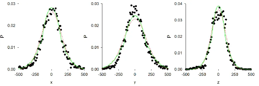
Figure 1. Analysis of a male-only swarm with 22 individuals (ref. Males08292120).
Distribution, P, of distances of each individual from the swarm centre. Telemetry data (●).
q-Gaussian ansatz (green line). Shown for comparison is the best fit q-Gaussian (red-line). The
Akaike weights for the q-Gaussians are 1.00, 1.00 and 1.00.
10
Figure 2. Analysis of a male-only swarm with 22 individuals (ref. Males08292120).
Distribution, P, of distances of each individual from the swarm centre. Telemetry data (●).
Best fit q-Gaussian (green line). Shown for comparison is the best fit Gaussian (red-line).
The Akaike weights for the q-Gaussians, are 1.00, 1.00 and 0.00.
11
Figure 3. Analysis of a male-only swarm with 7 individuals (ref. Males08252010a).
Distribution, P, of distances of each individual from the swarm centre. Telemetry data (●).
Best fit q-Gaussian (green line). Shown for comparison is the best fit Gaussian (red-line).
210