Characterisation of Field-of-View for Energy
Efficient Application-Aware Visual Sensor Networks
Anas Amjad,
Student Member, IEEE,
Mohammad Patwary,
Senior Member, IEEE,
Alison Griffiths
and Abdel-Hamid Soliman,
Member, IEEE
Abstract—Energy consumption is one of the primary concerns in a resource constrained Visual Sensor Network. The existing Visual Sensor Network design solutions under particular resource constrained scenarios are application specific; whereas the degree of sensitivity of any of these resource constrains (e.g. energy etc) varies from one application to another. This limits the implementation of the existing energy efficient solutions within a Visual Sensor Network node which may be considered to be a part of a heterogeneous network. The heterogeneity of image capture and processing within a Visual Sensor Network can be adaptively reflected with a dynamic Field-of-View realisation. This is expected to allow the implementation of a generalised energy efficient solution to adapt with the heterogeneity of the network. In this paper, an energy efficient Field-of-View characterisation framework is proposed which can support a diverse range of applications. The context of adaptivity in the proposed Field-of-View characterisation framework is considered to be: a) sensing range selection; b) maximising spatial coverage; c) adaptive task classification and d) minimising the number of required nodes. Soft decision criteria is exploited and it is observed that for a given detection reliability, the proposed framework provides energy efficient solutions which can be implemented within heterogeneous networks. It is also found that the proposed design solution for heterogeneous networks leads to 49.8%energy savings compared to the trivial design solution.
Index Terms—Energy optimisation, field-of-view characteri-sation, resource optimicharacteri-sation, sensing range estimation, task classification, visual sensor networks.
I. INTRODUCTION
A
Wireless Sensor Network (WSN) consists of a group of sensor nodes with sensing, processing and communica-tion capabilities. In tradicommunica-tional WSNs, sensors generally pro-vide coverage in all directions to collect scalar measurements as 1D data, for example: temperature, pressure, humidity etc that limits their suitability to many applications [1]. In order to enhance WSN’s suitability for a wider range of applications, its traditional sensors are replaced by visual sensors resulting in a network suitable for a new scope of applications known as a Visual Sensor Network (VSN). In a VSN, each node captures image data that can be processed locally to extract relevant information (such as visual features) and it collaborates with other nodes in the network [2]. VSNs are used in surveillance [3, 4], environmental monitoring [5, 6], assisted living and tele-healthcare [7, 8] applications. Visual sensors within aManuscript received April 24, 2015; revised January 20, 2016; accepted January 21, 2016.
The authors are with the Faculty of Computing, Engineering and Sciences, Staffordshire University, Stoke-on-Trent, UK (e-mail: [email protected]; [email protected]; [email protected]; [email protected]).
VSN employ directional sensing to provide pixel based mea-surements as a 2D dataset and they require a large bandwidth to transmit image data. The 3D viewing volume of a visual sensor is known as its Field-of-View (FoV) [2]. During the VSN design phase, some image processing algorithms require precise knowledge of the FoV. The fundamental differences between a traditional WSN and a VSN make the deployment of the latter more challenging as compared to the former. Furthermore, due to the directional sensing nature of visual sensors, the existing WSN design solutions are not suitable for VSNs.
In order to explore the challenges in more detail, consider a VSN deployed at a remote location for a surveillance ap-plication such as face detection, object detection and tracking etc. Since a power source may be unavailable, all nodes are assumed to be battery powered therefore the network lifetime is limited. This imposes tight constraints on energy consump-tion and data storage capacity within a VSN. Furthermore, the aforementioned surveillance tasks vary in terms of complexity and desired reliability. Therefore, the characterisation of FoV and task classification to provide an energy efficient design solution is an important and challenging problem in VSNs.
This paper is focused on the FoV characterisation and task classification to obtain an optimised VSN configuration for resource constrained scenarios. The configuration of a VSN considered in this paper is given by: a) the sensing range of the nodes and b) the allocation of sensing and processing tasks to the nodes which are part of a heterogeneous network. The contributions of this paper are summarised as follows:
1) A generalised FoV characterisation framework for ho-mogeneous and heterogeneous VSNs is proposed as a function of the required minimum object pixel oc-cupancy, maximum allowable error tolerance and de-sired image quality. The proposed FoV characterisation framework provides the system design engineers with a resource trade-off model while obtaining an optimised sensing range of a visual sensor node for any given application.
2) Considering the heterogeneity of the modern VSNs, an adaptive task classification scheme is proposed for the distribution of tasks between the nodes providing a trade-off model for reliability and energy efficiency. The proposed scheme provides solutions to the task classification problem feasible for implementation in resource constrained scenarios.
tech-niques is presented. The proposed framework, when employed with the proposed task classification and soft decision based sensing range selection schemes resulted in an optimised VSN configuration by maximising the spatial coverage, reducing the energy consumption and increasing the network lifetime without compromising on the desired reliability. Analysis of the energy effi-ciency of the proposed framework validates its suitability for a diverse range of applications
The rest of the paper is organised as follows; Section II explores the existing solutions for VSN design and their limitations, Section III presents the visual sensor 3D projection model. Section IV introduces the proposed FoV characterisa-tion framework. Seccharacterisa-tion V describes the experimental setup and presents the results. Section VI provides an analysis of the proposed framework’s energy efficiency. Section VII presents an analysis of system failure and finally, Section VIII provides the concluding remarks.
II. RELATEDWORK
In the last decade, researchers have been actively engaged in VSN coverage, design and optimisation problems. In [9], an unsupervised scheme is proposed to identify the overlapping FoV for the estimation of network topology in large VSNs. A mathematical model is proposed in [10] to solve VSN coverage problem by deploying each node sequentially and removing the overlapping nodes. Closed form solutions for VSN coverage estimation problem are proposed in [11] and [12] for homogeneous and heterogeneous VSNs respectively. The latter approach also considers the visual occlusions and boundary effect. A visual feature extractor, BRISKOLA (Bi-nary Robust Invariant Scalable Keypoints Optimized for Low-power ARM architectures), is proposed in [13] by optimising BRISK [14] for ARM architectures. The proposed approach can also be used in resource constrained VSNs. Ye et al. [15] proposed an energy-aware packet interleaving scheme for robust transmissions within VSNs to improve the end-to-end image transmission quality and prolong the network lifetime. In [16], Dai et al. proposed a routing algorithm by integrating correlation-aware inter-node differential coding and load balancing schemes. The proposed approach min-imises the sensor network’s energy consumption under certain constraints. Authors in [17] proposed camera scheduling and energy allocation schemes to maximise a VSN’s lifetime. Kim et al. [18] proposed an energy efficient scheme to maximise the data quality and lifetime of solar-powered VSNs. A VSN lifetime maximisation strategy is proposed in [19] that opti-mises the source rates, encoding powers and routing schemes to prolong the network’s lifetime. Authors in [20] proposed an energy efficient relaying scheme for data packets transmission within the VSN to increase its lifetime.
Although the existing work in literature addresses several key issues relating to VSNs such as FoV identification, cov-erage estimation, feature extraction, camera scheduling and transmission; it is found that the existing solutions are appli-cation specific under particular resource constrained scenarios. Furthermore, many existing solutions have limited application
capabilities as they assume a homogeneous network during the design phase. In this paper, an energy efficient FoV character-isation framework is proposed that exploits the heterogeneity of the network to obtain a design solution suitable for a diverse range of applications.
III. VISUALSENSOR3D PROJECTIONMODEL
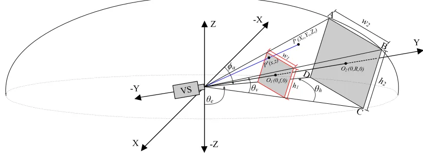
The 3D projection model of a visual sensor VS within a spherical sector is shown in Fig. 1. VS employs directional sensing and transforms a projection of the 3D scene fromR3to a 2D image plane inR2. In this model, the projection of the 3D scene points onto a physical 2D image plane is characterised by the pinhole camera model. In reality, the physical image plane lies inside the visual sensor behind its centre. The light rays hit the image plane through a pinhole and create an upside down image of the scene within the FoV. In order to simplify the mathematical model, it is assumed that the physical image plane lies infront of the sensor’s centre and provides the same image with respect to the scene within the FoV. The visual sensor covers a certain part of the spherical area of interest. The region within the sensor’s 3D FoV is described by the horizontal FoV (θh)and the vertical FoV (θv)of the sensor; whereθhandθvare the angular extents of the scene measured horizontally and vertically by the sensor respectively.
In Fig. 1, sensor VS is located at the origin of the cartesian coordinate system i.e. (0,0,0) and the sensor’s optical axis overlaps onto the y-axis with X = 0 and Z = 0. Within the context of a homogeneous VSN, where N sensor nodes are present, each sensor node VSu (u={1,2,3, . . . , N}) is identified by its location which is described by the cartesian coordinates (Xu, Yu, Zu), azimuth angle φa and elevation angle θe. These parameters define sensor distribution within the network and are tuned to fit the respective areas of interest within each sensor’s FoV. The originO2 of the ABCD-plane intersects the y-axis at (0, R,0); where R is the distance between the visual sensor and the ABCD-plane and is known as the sensing range, w2 is the width of the ABCD-plane and h2 is its height. For a target object, the sensing range spans from Rmin to Rmax for a certain acceptable level of sharpness. Varying R affects the sensor’s coverage area due to the change in ABCD-plane dimensions. Therefore, R is a key parameter for FoV characterisation. The width and height of the physical image plane are represented by w1 and h1 respectively. The physical distance f ∈ R+ between the sensor’s optical centre and the image plane is known as
the focal length. Each sensor maps P ×Q pixels onto the
image plane, where P ×Q is known as the resolution of the sensor. High resolution sensors are capable of observing a large area within their FoVs and result in reduction of the number of sensors required for full coverage. However, such sensors may increase the overall network design cost. Therefore, the selection of sensors for VSN design requires careful consideration of all the aforementioned parameters.
IV. PROPOSEDFOV CHARACTERISATIONFRAMEWORK
Fig. 1: Visual sensor’s 3D projection model.
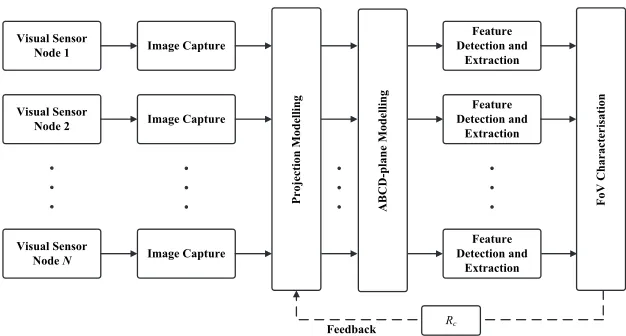
Based on the type of VSN, there are two approaches for its design and calibration: (i) Approach I for homogeneous sensor networks shown in Fig. 2a (ii) Approach II for heterogeneous sensor networks shown in Fig. 2b. The proposed framework consists of image capture, projection modelling, ABCD-plane modelling, adaptive task classification (for heterogeneous net-works), feature detection, extraction and FoV characterisation which are described in the following sections.
A. Image Capture
Each sensor VSucaptures an imageIuof dimensionP×Q which is a function of the following parameters: the rangeR, the horizontal FoVθh and the vertical FoV θv.
Iu=F(R, θh, θv) (1)
B. Projection Modelling
As mentioned earlier, a visual sensor projects 3D scene points onto its image plane. Volume V of the scene within the sensor’s FoV projected onto its image plane is given by,
V = 4R
3sinθhsinθv
3(1 + cosθh)(1 + cosθv) (2)
In order to characterise sensor’s coverage, FoV (θh, θv) is required to be known. The projection modelling approach is different for homogeneous and heterogeneous networks, as discussed in the following sections.
(i) Homogeneous Networks (Approach I): A homogeneous
sensor network has identical nodes in terms of their sensing parameters and hardware capabilities. Using the following equations [21], FoV (θh, θv) is calculated with prior knowl-edge of the sensor specifications.
θh= 2 arctan
w1
2f
(3)
θv= 2 arctan
h1
2f
(4)
(ii) Heterogeneous Networks (Approach II): A
heteroge-neous network has two or more types of nodes in terms of their sensing parameters and hardware capabilities. The nodes with lower specifications are less costly and consume less energy. On the other hand, the nodes with higher specifications can perform tasks with higher reliability but consume more energy and cost more. Keeping a certain reliability level in a heterogeneous network, few higher specification nodes can be used in each cluster along with the lower specification nodes to reduce the overall network cost.
In the case of using a variety of sensing nodes within the network, any of the following sensor specifications: (w1, h1) and (f) may be unknown and FoV (θh, θv) cannot be calculated through Approach I. For such case, an alternative approach is presented for calculating the FoV of each type of sensor node using the following equations,
θh= 2 arctanw2 2R
(5)
θv= 2 arctan
h2
2R
(6)
This method requires an experimental setup (described later in Section V) which utilises a known reference distanceR=
Rref for FoV calculation.
C. ABCD-plane Modelling
Onceθh and θv are known, the dimension of the ABCD-plane is calculated for a range of values of R i.e. Rmin to Rmax using the following equations,
w2= 2Rtan
θh
2
(7)
h2= 2Rtan
θv
2
(8)
D. Adaptive Task Classification
Visual Sensor Node 1
Visual Sensor Node 2
Visual Sensor Node N
Image Capture
Image Capture
Image Capture
Feature Detection and
Extraction Feature Detection and
Extraction
Feature Detection and
Extraction
Rc
Feedback
ABCD-plane Modelling FoV Characteri
sati
on
Projection Modelling
(a) FoV Characterisation (Approach I) for homogeneous VSNs
Image Capture
Feature Detection and
Extraction
Rc , r
Feedback Node 1
Node 2
Node n1
Visual Sensor
Class
1
Node 1 Node 2
Node n2
Visual Sensor
Class 2
Image Capture
Feature Detection and
Extraction
Node 1 Node 2
Node nk
Visual Sensor
Class
k
Image Capture
Feature Detection and
Extraction
Projection Modelling ABCD-plane Modelling
Adaptive Task Classi
fication
FoV Characteri
sati
on
(b) FoV Characterisation (Approach II) for heterogeneous VSNs
Fig. 2: Proposed FoV Characterisation Framework for Energy Efficient VSNs.
sensing and processing tasks assigned to each visual sensor class based on its sensing capabilities. Adaptive task classifi-cation is employed by the FoV characterisation framework to enhance the intelligence of heterogeneous networks. Consider a heterogeneous sensor network with k sensor classes; each sensor is denoted by VSl,j such that l = {1,2,3, . . . , k} represents the sensor class andj={1,2,3, . . . , n}represents nl sensors belonging to a sensing class l. Letn denotes the maximum number of sensors belonging to a particular sensing class given by n= max{nl|l= 1,2,3, . . . , k}. The sensors within the VSN can be represented by,
VS=
VS1,1 VS1,2 . . . VS1,n
VS2,1 VS2,2 . . . VS2,n
..
. ... . .. ...
VSk,1 VSk,2 . . . VSk,n
Assume the sensor network is divided into clusters and each cluster head receives control signals from the cluster nodes to
determine whether they are active or inactive. VSl,jis assigned a value based on the following condition,
VSl,j =
−1, if j > nl
1, if the sensor is active
0, if the sensor is inactive
(9)
Supposetrepresents the total sensing and processing tasks within the VSN. Let ani-dimensional task classification matrix
Tsuch thati={1,2,3, . . . , t} is given by,
T=
T1,1 T1,2 . . . T1,n
T2,1 T2,2 . . . T2,n
..
. ... . .. ...
Tk,1 Tk,2 . . . Tk,n
where eachTl,j is given by,
Tl,j =
(
1, ifithtask is assigned to sensor VSl,j
In the proposed approach, upto d√ke sensor classes are assigned anithtask; where(d e)refers to the ceiling function. Let T0i denotes the adaptive ith task classification matrix which optimises Ti for active sensing nodes within the VSN and is given by,
T0i=
1 2
h
Ti·VS+J i
(11)
where Jis a k×n all-ones matrix and (b c) refers to the floor function.
Feedback Rc and r are substituted in (2) to calculate the required 3D scene coverageVc ofksensor classes to perform ttasks and the chosen 3D scene coveragevofksensor classes respectively. Algorithm 1 presents the proposed adaptive task classification scheme that calculates T and then T0 in an optimised way.
E. Feature Detection and Extraction
Global colour histogram is used for object detection and feature extraction. It represents the distribution of colours within each captured image Ii of size P ×Q and is given by [22],
hc(b) =
P X
x=1 Q X
z=1 (
1, ifIi(x, z)is in binb
0, otherwise (12)
where a colour bin defines a region of particular colour. In this framework, histogram-based features have been extracted in YCbCr colour space as it distinguishes the lu-minance and chrolu-minance. The extracted features have been analysed and a range of values of Cb and Cr has been defined to detect a particular object of interest through image segmentation.
The probabilityP(E)of a pixel at location(x, z)belonging to an object of interest is given by,
P(E) =
(
1, if γl
Cb≤Cb≤γuCb∩γCrl ≤Cr≤γuCr
0, otherwise
(13) The pixels probabilities are indexed at their respective locations in the object segmentation matrix Sm. The object of interest is extracted from Ii by image segmentation using the following equation [23],
Sg=Ii.Sm (14)
where Sg is the segmented image and (.) refers to the dot product.
F. FoV Characterisation
The relationship between sensor’s resolution and ABCD-plane dimensions for a distance R is given by,
dh= P
w2 ; dv=
Q
h2 (15)
where dh is the horizontal and dv is the vertical density measured in pixels/mm.
As P and Q are constant, it is found that dh ∝ 1/w2 and dv ∝1/h2. Increasing the distance R increases w2 and
Algorithm 1 Adaptive task classification scheme for hetero-geneous networks
Require:
The number of: sensor classesk, sensors of each typenl, taskstrequired to be performed by the VSN; the required 3D scene coverage Vc of k sensor classes to perform t tasks and the chosen 3D scene coverage v of k sensor classes.
Ensure:
For∀ j∈ {1,2,3, . . . , n} and∀i∈ {1,2,3, . . . , t}
0< k X
l=1
T0(l, j, i)≤ d√ke
1: n←max{n1, n2, n3, . . . , nk} 2: VS←∅
3: s←[−1 1 0 0 0]
4: forl←1tok do
5: forj←1tondo
6: if j > nl then
7: VS(l, j)←s1
8: else ifsensor is activethen
9: VS(l, j)←s2
10: else ifsensor is inactive then
11: VS(l, j)←s3
12: end if
13: end for 14: end for 15: T←∅ 16: T0 ←∅
17: fori←1totdo
18: forl←1tokdo
19: s5←k−l+ 1
20: if Vc(s5, i)≥v(s5) &s4<d√kethen
21: T(s5,1:n, i)←s2
22: s4←s4+ 1
23: else
24: T(s5,1:n, i)←s3
25: end if
26: end for
27: T0i=
1
2
h
Ti·VS+J i
28: s4←0 29: end for 30: return T0
h2 which results in the reduction of horizontal and vertical density. IfR goes outside a certain range, the captured image may not provide sufficient feature descriptors. Hence, the need arises to propose a criteria for optimised range defined as
theField-of-View Characterisation Criteria(FoVCC). FoVCC
must ensure the presence of sufficient feature descriptors within the captured image as well as guarantee optimised utilisation of resources while maintaining a certain quality.
(i) Object Pixel Occupancy: The number of pixels (Opo)
an object of interest occupies in the image captured from a particular distance R is derived as,
Opo=A× P
2Rtan θh 2
× Q
2Rtan θv 2
(16)
where A is the area of the object inmm2. Let ξo defines the required minimum pixel occupancy for a particular applica-tion, the chosen rangeR1of a visual sensor must guarantee the criteria Opo≥ξo and it can be calculated using the following equation,
R1=
s
P×Q×A
4×Opo×tan θh 2
×tan θv 2
(17)
Table I provides the minimum object pixel occupancy required for various detection algorithms.ξofor face detection depends on the image size used to train the classifiers. The detection accuracy calculated on PETS 2005 data set in [24] withξo= 25for LOTS, SGM and MSM is 91.2%, 86.8%and 85.0%respectively.
TABLE I: Required minimum object pixel occupancy for various detection algorithms
Detection Method ξo
Viola-Jones face detector [25] 315 Lehigh Omnidirectional Tracking System (LOTS) [26] 25
Single Gaussian Model (SGM) [27] 25 Multiple Gaussian Model (MGM) [28] 25
(ii) Estimation Error: Increasing range R1 reduces the
object pixel occupancy Opo which may lead to detec-tion/estimation error. Hence, the need arises to provide a method for the estimation of maximum sensing range based on a certain acceptable error tolerance level. In order to propose such method, an application that estimates the detected object’s diameter from the acquired visual data is considered.
After feature detection, ifOpodenotes the number of pixels representing the detected object; the framework estimates pixels representing the diameterpd by,
pd= 2
r Opo
π (18)
The diameterde of the object is estimated by,
de= 4Rtan
θh 2 P r Opo
π (metres) (19)
If da is the actual measured diameter of the object of interest, the absolute percentage estimation error|εd|is given by,
|εd|=|da−de|
da ×100 (%) (20)
It is expected that as the range increases, the estimation error will increase. Let ξd defines the maximum acceptable estimation error in percentage for a particular application, the chosen rangeR2of a visual sensor must guarantee the criteria
|εd| ≤ξd.
Substituting (19) in (20), the range R2 can be calculated using the following equation,
R2= " r π Opo #" P da
4 tan θh 2
#"
1−|εd| 100
#
(21)
The above equation is valid for|εd| 6= 100%.
(iii) PSNR: Suppose image I1 of dimension P ×Q is
captured at a distance Rp which contains a particular object of interest. The aforementioned histogram-based feature ex-traction scheme is employed to extract the region of interest containing only the object under consideration in the form of image I01 of dimension P0 ×Q0. As I0
1 contains the object captured at distance Rp, the dimension Ps×Qs of image
Is containing the extracted object at distance Rs (such that Rs> Rp) is estimated by,
Ps=P0 w
Rp 2 wRs
2 !
; Qs=Q0 h Rp 2 hRs
2 !
(22)
where wRp
2 , w
Rs
2 , h
Rp
2 and h
Rs
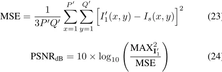
2 are calculated using (7) and (8). As Ps< P0 and Qs< Q0, the object captured and extracted at distance Rs appears smaller in size. In order to measure the quality,I01 andIsare compared to find the Peak Signal-to-Noise Ratio (PSNR) value. As PSNR requires both images to have the same size,Is is resized toP0×Q0. First, Mean Squared Error (MSE) is calculated and then the PSNR.
MSE= 1
3P0Q0 P0 X x=1 Q0 X y=1 h
I10(x, y)−Is(x, y) i2
(23)
PSNRdB= 10×log10
MAX2I0 1
MSE !
(24)
where MAX2I0
1 is the maximum possible pixel value in I 0 1. Let ξp defines the required minimum PSNRdB for a
par-ticular application, the chosen range R3 of a visual sensor must guarantee the criteria PSNRdB ≥ξp. As this method is
based on image quality assessment, an experiment needs to be conducted to find the rangeR3 from graph analysis which is discussed later in Section V.
Apart from PSNRdB, there are many other image quality
assessment methods such as [29, 30] that can be used with the proposed FoV characterisation framework based on their respective confidence bounds for sensing range estimation.
The selection of one or more characterisation methods depends on the application and the design criteria. The applica-tion where design considers the detecapplica-tion method’s minimum pixel requirement, object pixel occupancy based method is used. If the design criteria depends on a particular tolerance level, then estimation error based method is used. The design considering image quality utilises the PSNR based method.
LetRc defines the chosen value of sensor’s range, the FoV Characterisation Criteria (FoVCC) is proposed as,
Rc=
R1 ifOpo≥ξo
R2 if|εd| ≤ξd
R3 if PSNRdB≥ξp
The sensing range for applications where the design engi-neer utilises more than one characterisation method is selected by Rc= min{R1, R2, R3}. The designed VSN’s FoV is said to be optimised based on the following criteria,
(
Rc =R1∪Rc =R2∪Rc =R3 Optimised
Rc 6=R1∩Rc 6=R2∩Rc 6=R3 Unoptimised (26)
G. Adaptive Range Selection
(i) Hard decision based sensing range selection: In
homo-geneous network design that considersttasks to be performed within the VSN, sensing range {Rc(i) | i= 1,2,3, . . . , t} is required to be calculated for each task. The sensing range Rc can be obtained by hard decision as shown below,
Rc= min{Rc(1), Rc(2), Rc(3), . . . , Rc(t)} (27)
The chosen sensing range Rc is the feedback to projection modelling.
In the case of heterogeneous network design, Rc of di-mensionk×t is the feedback to projection modelling which provides the estimated sensing range ofksensor classes fort tasks.
Rc=
Rc(1,1) Rc(1,2) . . . Rc(1,t)
Rc(2,1) Rc(2,2) . . . Rc(2,t)
..
. ... . .. ...
Rc(k,1) Rc(k,2) . . . Rc(k,t)
Sensing range r(l)can be calculated for each sensor class by hard decision as shown below,
r(l) = min{Rc(l,1), Rc(l,2), Rc(l,3), . . . , Rc(l,t)} (28)
The individual sensing range values for different sensor classes obtained through hard decision can be represented collectively by ras,
r= [r(1), r(2), . . . , r(k)]T (29) where [·]T refers to transpose. The proposed hard decision
based scheme is suitable for homogeneous networks as they have identical sensor nodes and hard decisions need to be made for sensing range selection. However, the hard deci-sion based scheme for heterogeneous networks does not take advantage of the multiple sensor classes present within the network. The approach provides the minimum range for each sensor class and does not prolong the network lifetime by maximising the sensing range. To maximise the sensing range and prolong the lifetime of heterogeneous networks, a soft decision based scheme for sensing range selection is proposed in the following section.
(ii) Soft decision based sensing range selection: A soft
decision based sensing range selection scheme is proposed in Algorithm 2 which calculates a suitable range r(·) for each sensor class based on the estimated Rc. The algorithm provides range r for k sensor classes by maximising it for
(k− d√ke)sensor classes.
Algorithm 2 Proposed soft decision based sensing range selection scheme for heterogeneous network design
Require:
The number of: sensor classes k, sensors of each type nl, tasks t required to be performed by the VSN; Rc providing the estimated sensing range ofksensor classes for t tasks.
Ensure:
For d√ke values of l ∈ {1,2,3, . . . , k} and ∀ i ∈ {1,2,3, . . . , t}
r(l)≤Rc(l,i) 1: s1=∅
2: forl←1tok do
3: s1← t X
i=1 Rc(l,i)
4: end for
5: s2←Sorts1 in ascending order 6: s3←First d
√
kevalues’ indices froms2 7: forl←1tok do
8: ifl∈s3 then
9: r(l)←min{Rc(l,1), Rc(l,2), Rc(l,3), . . . , Rc(l,t)} 10: else ifl /∈s3 then
11: r(l)← 1
t
×
t X
i=1 Rc(l,i)
12: end if 13: end for
14: return r
V. EXPERIMENTALSETUP ANDRESULTS A. Image Capture
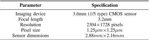
Specification of the visual sensor used for experiments is presented in Table II.
TABLE II: Visual sensor specification
Parameter Specification
Imaging device 3.6mm (1/5 type) CMOS sensor
Focal length 3.2mm
Resolution 2304×1728 pixels
Pixel size 1.25µm×1.25µm
Sensor dimensions 2.88mm×2.16mm
B. Projection Modelling utilising Approach I
Using Projection Modelling Approach I for homogeneous VSNs, after substituting focal length (f) and sensor dimen-sions (w1 × h1) in (3) and (4), the calculated values of horizontal and vertical FoVs are: θh = 48.39◦, θv = 37.25◦ respectively.
C. Projection Modelling utilising Approach II
Projection Modelling Approach II, they will be compared with those calculated from Projection Modelling Approach I. The experimental procedure is described in Table III.
TABLE III: Experiment 1 procedure
Procedure: Experiment 1
1: The visual sensor is placed near a wall at a certain heightht and a known reference distanceRrefwithout any tilt or pan. 2: A certain portion of the wall is captured within the sensor’s
FoV.
3: The widthw2and heighth2of the wall’s portion within the FoV are measured forRref.
4: Using (5) and (6),θhandθvare calculated.
5: Steps 1 to 4 are repeated for a set of values of Rref to guarantee the accuracy of the calculatedθhandθvvalues.
The experimental results for six cases have been sum-marised in Table IV; where each case is distinguished by its reference distanceRref.
TABLE IV: FoV calculation utilising Projection Modelling Approach II
Parameter Case Case Case Case Case Case Average
1 2 3 4 5 6
Rref 0.27m 0.30m 0.45m 0.68m 0.92m 1.91m
-w2 0.24m 0.27m 0.40m 0.61m 0.82m 1.72m
-h2 0.18m 0.20m 0.30m 0.46m 0.62m 1.29m
-ht 1.04m 1.04m 1.04m 1.04m 1.04m 1.04m
-θh 48.37◦ 48.38◦ 48.43◦ 48.41◦ 48.29◦ 48.48◦ 48.39◦
θv 37.11◦ 37.23◦ 37.29◦ 37.30◦ 37.16◦ 37.40◦ 37.25◦
φa 41.54◦ 41.54◦ 41.54◦ 41.54◦ 41.54◦ 41.54◦
-θe 52.75◦ 52.75◦ 52.75◦ 52.75◦ 52.75◦ 52.75◦
-Based on the experimental results it is found that the error for each case is negligible and by averaging the estimated values, the projection modelling approach II leads to accurate FoV measurements.
D. ABCD-plane Modelling
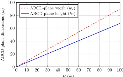
ABCD-plane modelling plays a vital role for FoV char-acterisation. As θh and θv have been calculated, extensive numerical simulations have been performed for ABCD-plane modelling utilising (7) and (8) for a range of values ofR. The simulation results are presented in Fig. 3. From the results, it is found that increasing the sensing range increases the ABCD-plane’s width (w2) and height (h2) as well. In this case, w2> h2 for any value ofR due to the fact thatθh> θv.
E. Feature Detection and Extraction
Using the global colour histogram, the probabilityP(E)of a pixel at location(x, y)belonging to the object of interest is found to be,
P(E) =
(
1, if 43≤Cb≤90∩138≤Cr≤159
0, otherwise (30)
After dataset creation (discussed in the following section) probability P(E) can be used for feature detection and ex-traction.
0 10 20 30 40 50 60 70 80 90 100
0 20 40 60 80 100
R(m)
ABCD-plane
dim
ensions
(
m
) ABCD-plane width (w2)
ABCD-plane height (h2)
Fig. 3: ABCD-plane modelling.
F. FoV Characterisation
Although the FoV characterisation depends on several fac-tors, sensing range (R) is the key parameter for the characteri-sation process. The sensing range estimation and optimicharacteri-sation requires practical measurements and simulations. The experi-mental procedure for these calculations is described in Table V.
TABLE V: Experiment 2 procedure
Procedure: Experiment 2
1: A particular type of feature needs to be considered based on the desired application. In this experiment, colour features are considered.
2: Images of objects under consideration are captured for a range of values ofR.
3: The captured images are processed to classify those contain-ing sufficient colour feature descriptors.
4: A particular value ofRcis chosen for VSN design based on the FoVCC.
In order to estimate the sensing range for optimised FoV characterisation, a dataset is created by capturing objects for a range of values of R i.e. 0.25m to 9.55m. Sensing range can be estimated for optimised FoV characterisation using one or a combination of the following parameters: object pixel occupancy, estimation error, PSNR. The experimental and simulation results for FoV characterisation are presented and analysed in the following sections.
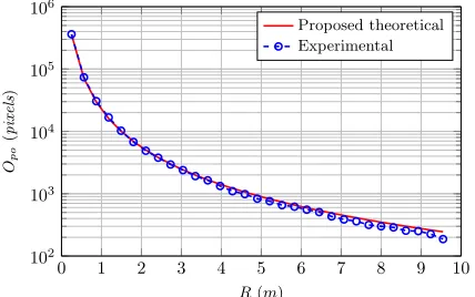
(i) Object Pixel Occupancy: Fig. 4 shows a comparison of
0 1 2 3 4 5 6 7 8 9 10 102
103
104
105
106
R(m)
Opo
(
pixels
)
Proposed theoretical Experimental
Fig. 4: A comparison of theoretical and experimental values of object pixel occupancy.
0 1 2 3 4 5 6 7 8 9 10
5 5.5 6 6.5 7 7.5 8
R(m)
Diameter
(
cm
)
Actual Diameter (da) Estimated Diameter (de)
Fig. 5: A comparison of actual and estimated diameter for different sensing range values.
0 1 2 3 4 5 6 7 8 9 10
0 3 6 9 12 15
R(m)
|
εd
|
(%)
Fig. 6: Estimation error for different sensing range values.
0 1 2 3 4 5 6 7 8 9 10
20 25 30 35 40 45 50
R(m)
PSNR
(d
B
)
Fig. 7: PSNR estimation for different sensing range values.
As an example, a face detection application [25] requires object pixel occupancy to be atleast 315 pixels i.e.Opo≥315, the acceptable sensing range in that case will beR1≤4.05m.
(ii) Estimation Error: Using (19), Fig. 5 presents a
compar-ison of actual and estimated diameter for images captured for a range of values ofR. The absolute percentage estimation error
|εd|is shown in Fig. 6. It has been noticed from Fig. 6 that as the range increases, the estimation error increases. This is due to the fact that the object of interest appears too small beyond a certain range which leads to inaccurate feature detection and extraction results. As an example, suppose a particular application can tolerate maximum 6% error i.e. |εd| ≤ 6%, the acceptable sensing range will be R2≤6.76m.
(iii) PSNR: This method utilises an image quality
assess-ment technique for FoV characterisation. Fig. 7 shows the estimated PSNRdB for a range of values ofRand it has been
noticed that as the range increases, the PSNRdB decreases.
As PSNRdB is an index for image quality assessment, this
method can assist the design engineer to tune the network for a suitable image quality. As an example, an image transmission application [31] requires PSNRdB to be atleast 30dB i.e.
PSNRdB ≥ 30dB, the acceptable sensing range in that case
will beR3≤9.55m.
G. Adaptive Range Selection
(i) Homogeneous Networks: Consider a homogeneous
net-work design for a surveillance application that requirest= 2
tasks to be performed within the VSN i.e. face detection [25] (Task I) and occluded target surveillance and tracking [26] (Task II). Suppose a medium resolution sensor with the following parameters: P ×Q = 640 ×480, θh = 48.39◦
and θv = 37.25◦ is selected for the VSN design. Let the object pixel occupancy based characterisation method is used with required minimum Opo = 315 and Opo = 25 for Task I and Task II respectively. The area (A) to be considered for detection is found to be 406cm2for Task I and 3922.6cm2for Task II. By substituting these parameters in (17), the sensing range estimated for Task I isRc1= 8.09mand for Task II is Rc2= 89.21m. According to the hard decision based sensing range selection method for homogeneous networks, the chosen sensing range Rc is min{Rc1, Rc2} i.e. Rc = 8.09m. The chosen rangeRc is a feedback to projection modelling and it is also used to find the number of active sensor nodes (Na) required within the VSN to perform the desired tasks.
(ii) Heterogeneous Networks: Now consider a
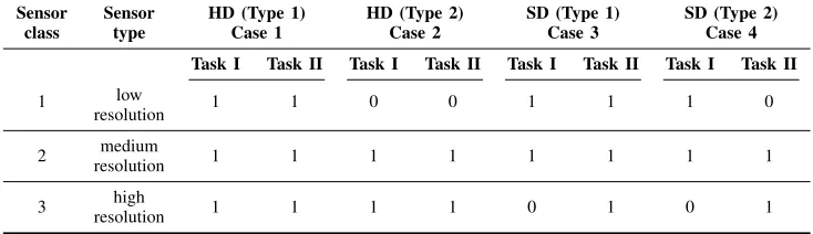
TABLE VI: A comparison of task classification using four different cases for a network consisting of k = 3 sensor classes performing t= 2 tasks
Sensor Sensor HD (Type 1) HD (Type 2) SD (Type 1) SD (Type 2) class type Case 1 Case 2 Case 3 Case 4
Task I Task II Task I Task II Task I Task II Task I Task II
1 low 1 1 0 0 1 1 1 0
resolution
2 resolutionmedium 1 1 1 1 1 1 1 1
3 high 1 1 1 1 0 1 0 1
resolution
P×Q= 2304×1728. The horizontal FoV (θh) and the vertical FoV (θv) are assumed to be same for k = 3 sensor classes and are given byθh= 48.39◦andθv = 37.25◦. Again, object pixel occupancy based characterisation method is considered with the same Opo and A values described earlier for the homogeneous network scenario.
In this case, the matrix Rc which is the feedback to projection modelling is found to be,
Rc =
Rc11 Rc12
Rc21 Rc22
Rc31 Rc32
=
4.05 44.60 8.09 89.21 29.12 321.16
In this design solution, Rc is calculated in metres. Using the hard decision based sensing range selection scheme, the chosen range is calculated (in metres) to be
r = [r(1), r(2), r(3)]T = [4.05,8.09,29.12]T. The range computed using the soft decision based scheme is r = [4.05,8.09,175.14]T.
This vector r is also a feedback to projection modelling. It can be observed from the comparison ofr computed using the hard and soft decision based approaches that the latter maximises the sensing range for (k − d√ke)
k=3 sensor classes. The hard decision based approach computed r(3)to be 29.12mwhereas, the soft decision based scheme calculated r(3)to be 175.14m. This shows that the soft decision based scheme maximised the range approximately 6 times compared to the hard decision based approach.
H. Sensor’s 3D Coverage Estimation
The sensor’s 3D coverage volume can be calculated from (2) by substitutingθh andθv for a suitable sensing range R. In the case of homogeneous sensor networks, feedback Rc is utilised for projection modelling. Considering the homo-geneous network design solution presented in the previous section and using (2), the chosen sensing range Rc= 8.09m leads to 3D coverage volume 106.90m3.
On the other hand, heterogeneous networks require feedback
Rc and r for projection modelling. Considering the hetero-geneous network design solution presented earlier and using (2), feedback Rc leads to the following required 3D scene coverageVc(inm3) ofk= 3sensor classes to performt= 2 tasks.
Vc=
13.41 1.79×10⁴
106.90 1.43×10⁵
4.99×10³ 6.69×10⁶
After calculating r using the hard decision based scheme, the chosen 3D scene coverage v (in m3) of k = 3 sensor classes is found to bev=
13.41,106.90,4.99×103T . Sim-ilarly, after calculatingrusing the soft decision based scheme, the chosen 3D scene coverage v (in m3) of k = 3 sensor classes is found to bev=
13.41,106.90,1.08×106T .
I. Adaptive Task Classification
In the proposed adaptive task classification scheme for het-erogeneous networks, upto d√kesensor classes are assigned a certain task. Considering the heterogeneous design solution presented earlier, d√ke
k=3 evaluates to the allocation of 2 sensor classes for each task. The proposed scheme utilisesVc andv (calculated from the soft decision based sensing range selection scheme) for task classification.
In order to analyse the proposed task classification scheme, four different cases are compared. These are being hard decision based approach without d√ke upperbound (case 1), hard decision based approach withd√keupperbound (case 2), soft decision based approach withoutd√keupperbound (case 3) and soft decision based approach with d√ke upperbound (case 4).
Table VI summarises the task classification results for these cases where ‘Task I’ refers to face detection, ‘Task II’ refers to occluded targets surveillance and tracking, ‘1’ refers to an allocated task and ‘0’ refers to an unallocated task.
Case 1 for task classification leads to a trivial solution where each sensor class has to perform every single desired task. Clearly, this is not a desired solution for VSN design. Although, case 2 provides a better solution as compared to case 1, it totally neglects the sensor class 1 by not allocating even a single task. It can be noticed that the task classification solution from case 2 will always neglect (k− d√ke)sensor classes due to the hard decision. The solution obtained from case 3 is somewhere between the solutions of case 1 and case 2. Utilising the proposed soft decision based approach with
VI. ENERGYEFFICIENCY OF THEPROPOSEDFRAMEWORK Consider a visual sensor network that requires Na active nodes to cover an area of size100×100m2. The number of nodesNarequired to be active depends on: the chosen sensing range Rc for homogeneous networks, or the chosen sensing range rof ksensor classes for heterogeneous networks.
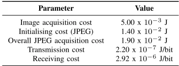
To validate the proposed framework which provides opti-mised energy consumption within certain desired confidence bounds, an energy-measurement testbed employed in [32] is considered. Each visual node within the testbed consists of a multimedia subsystem and a radio subsystem. The testbed’s parameters are listed in Table VII.
TABLE VII: Energy-measurement testbed’s parameters
Parameter Value
Image acquisition cost 5.00 x10⁻³J Initialising cost (JPEG) 1.40 x10⁻²J Overall JPEG acquisition cost 1.90 x10⁻²J Transmission cost 2.20 x10⁻⁷ J/bit
Receiving cost 2.92 x10⁻⁶ J/bit
SupposeEAcq,ET x andERx denote the energy consump-tion of a single visual node to acquire, transmit and receive a single image frame respectively. Consider a scenario where each node within the VSN acquires, transmits and receives one image frame, the overall acquisition, transmission or receiving cost is given by,
˜
Eq =Na×Eq ; q∈ {Acq, T x, Rx} (31)
The total energy consumption within the VSN will be,
Ec=Na×(EAcq+ET x+ERx) (32)
The energy efficiency of the proposed framework for both homogeneous and heterogeneous networks is discussed in the following sections.
A. Homogeneous Networks
Consider a homogeneous network for a surveillance appli-cation that utilises a sensor with the following parameters: P ×Q = 320×240, θh = 48.39◦ and θv = 37.25◦. A comparison of image acquisition, transmission and receiving costs for different sensing range values is shown in Fig. 8.
0 10 20 30 40 50 60 70 80 90 100
10−2
10−1
100
101
102
103
104
105
106
R(m)
Energy
consum
ption
(
Joules
) Receiving cost
Transmission cost
JPEG image acquisition cost
Fig. 8: A comparison of JPEG image acquisition, transmission and receiving cost for different sensing range values .
It is found from the results that increasing the sensing range results in less number of required active nodes leading to reduced energy consumption. However, if the sensing range goes beyond a certain threshold, the sensor may not provide accurate feature descriptors and may lead to miss detections. In that case, the proposed framework can be used for application-aware sensing range estimation during the VSN design and calibration process. It maximises the spatial coverage leading to the reduced energy consumption configuration without compromising on the desired accuracy. Moreover, reducing the energy consumption will prolong the network’s lifetime.
Table VIII lists the estimated sensing range for various applications based on certain criteria along with the number of required active nodesNa and the total energy consumption Ec within the VSN. The applications are listed in descending order of their energy consumption. The results show that the application-aware proposed FoV characterisation framework estimates the sensing range based on the desired criteria to maximise the spatial-coverage within the VSN and thus optimises the energy consumption. Suppose the lifetime of a VSN employing face detection algorithm is LT. It is evident from the results that the proposed approach leads to 2.78 −
112.92 times increased VSN lifetime for other applications in comparison with the first. The proposed framework has also optimised the number of required active nodes Na leading to reduced energy consumption configuration. The LOTS method proposed in [26] for occluded targets surveillance and tracking finds its applications in military where energy efficiency is highly desirable. As shown in the results, utilising the proposed approach with LOTS has resulted in optimised energy consumption. Hence, the application-aware sensing range estimation from the proposed approach makes it suitable for a wide range of applications and it can be utilised to design and calibrate an energy efficient VSN.
B. Heterogeneous Networks
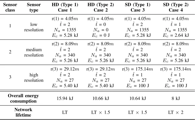
Heterogeneous networks provide much more flexibility to the design engineer compared to the homogeneous networks due to the presence of different types of sensor nodes within the network. The analysis of energy efficiency presented in the previous section for homogeneous networks considered the de-sign solution for four different applications. For heterogeneous networks, supposeˆtrepresents the number of tasks allocated to a sensing class; the task classification solutions obtained from four different cases given in Table VI are used to analyse the energy efficiency of the proposed framework and the results are presented in Table IX.
TABLE VIII: Application-aware sensing range estimation and energy consumption
Application Characterisation Criteria Range and Gain Network
method energy lifetime
Face detection [25] object pixel occupancybased Opo≥315
R1= 4.05m
− LT
Na= 1355 Ec= 2.64 kJ
Feature extraction & size
estimation estimation error based |εd| ≤6%
R2= 6.76m
64.06% LT×2.78 Na= 487
Ec= 948.78 J
Image transmission using
IEEE 802.15.4a [31] PSNR based PSNRdB≥30dB
R3= 9.55m
81.99% LT×5.55 Na= 244
Ec= 475.36 J
Occluded targets surveillance & tracking [26]
object pixel occupancy
based Opo≥25
R1= 44.60m
99.11% LT×112.92
Na= 12
Ec= 23.38 J
TABLE IX: Analysis of the energy efficiency of the proposed framework for heterogeneous network design
Sensor Sensor HD (Type 1) HD (Type 2) SD (Type 1) SD (Type 2) class type Case 1 Case 2 Case 3 Case 4
1
r(1) = 4.05m r(1) = 4.05m r(1) = 4.05m r(1) = 4.05m
low ˆt= 2 ˆt= 0 ˆt= 2 ˆt= 1
resolution Na= 1355 Na= 0 Na= 1355 Na= 1355 Ec= 5.28 kJ Ec= 0 J Ec= 5.28 kJ Ec= 2.64 kJ
2
r(2) = 8.09m r(2) = 8.09m r(2) = 8.09m r(2) = 8.09m
medium ˆt= 2 ˆt= 2 ˆt= 2 ˆt= 2
resolution Na= 340 Na= 340 Na= 340 Na= 340 Ec= 5.26 kJ Ec= 5.26 kJ Ec= 5.26 kJ Ec= 5.26 kJ
3
r(3) = 29.12m r(3) = 29.12m r(3) = 175.14m r(3) = 175.14m
high ˆt= 2 ˆt= 2 ˆt= 1 ˆt= 1
resolution Na= 27 Na= 27 Na= 27 Na= 27
Ec= 5.40 kJ Ec= 5.40 kJ Ec= 100 J Ec= 100 J
Overall energy
15.94 kJ 10.66 kJ 10.64 kJ 8 kJ
consumption
Network
LT LT×1.5 LT×1.5 LT×2
lifetime
VII. ANALYSIS OFSYSTEMFAILURE
After the design process, the VSN is expected to perform tasks within a certain confidence bound. Let ζl to ζu be the dynamic PSNR range in dB for a particular application andδ1= antilog−ζu
10
−antilog− ζl 10
be the dynamic difference. Supposeλtdenotes the threshold for system quality assessment representing the desired PSNR in dB. The proba-bility that a system with qualityβ (representing the achieved PSNR in dB) will fail to perform a certain task is derived as,
P(λt> β) =
0 if λt< β
δ2
δ1 if λt≥β
(33)
whereδ2= antilog−λt 10
−antilog−10β
Fig. 9 shows an analysis of system failure for several values ofλt. It can be observed from the graph that the system failure probability is maximum whenλtandβare at the opposite ends of the dynamic PSNR range. The system failure probability reduces when λt and β lies between the dynamic range and minimises to zero when λt< β.
24 27 30 33 36 39 42
0 0.2 0.4 0.6 0.8 1
β(dB)
System
failure
probabilit
y
λt= 42 dB
λt= 33 dB
λt= 30 dB
Fig. 9: Analysis of system failure.
VIII. CONCLUSION
sensing range of a visual sensor node. For any given applica-tion, the proposed solution for FoV characterisation enhances the spatial coverage, optimises the energy consumption and increases the lifetime in homogeneous networks. This paper also proposes adaptive task classification and soft decision based sensing range selection schemes for heterogeneous net-works. The configuration of heterogeneous network obtained by utilising the proposed FoV characterisation framework with the task classification and sensing range selection schemes for a surveillance application resulted in 49.8% energy savings compared to the trivial design solution. Based on the required and achieved quality of the captured image by a visual sensor node, an analysis of system failure is presented to predict and minimise the network failure probability. The energy efficiency of the proposed FoV characterisation framework demonstrates that it can be utilised during the network design and calibration phase to achieve an application-aware solution. Furthermore, the proposed framework provides simplified direction to future research within the context of homogeneous and heteroge-neous VSN design. For the future extension of this work, the authors intend to develop generalised adaptation models of feature detection and extraction schemes for realisation with the proposed framework.
REFERENCES
[1] Y. Charfi, N. Wakamiya, and M. Murata, “Challenging issues in visual sensor networks,” IEEE Wireless
Com-munications, vol. 16, no. 2, pp. 44–49, April 2009.
[2] S. Soro and W. Heinzelman, “A survey of visual sensor networks,”Advances in Multimedia, vol. 2009, 2009. [3] N. B. Bo et al., “Human mobility monitoring in very
low resolution visual sensor network,” Sensors, vol. 14, no. 11, pp. 20 800–20 824, 2014.
[4] Y. Cho, S. O. Lim, and H. S. Yang, “Collaborative occupancy reasoning in visual sensor network for scal-able smart video surveillance,” IEEE Transactions on
Consumer Electronics, vol. 56, no. 3, pp. 1997–2003,
Aug 2010.
[5] A. Filonenko and K.-H. Jo, “Visual surveillance with sensor network for accident detection,” in 39th Annual Conference of the IEEE Industrial Electronics Society
(IECON), Nov 2013, pp. 5516–5521.
[6] N. Ahmad, K. Khursheed, M. Imran, N. Lawal, and M. O’Nils, “Modeling and verification of a heteroge-neous sky surveillance visual sensor network,”
Interna-tional Journal of Distributed Sensor Networks, vol. 2013,
2013.
[7] F. Deboeverie, J. Hanca, R. Kleihorst, A. Munteanu, and W. Philips, “A low-cost visual sensor network for elderly care,”SPIE NEWSROOM, no. 1, 2014.
[8] M. Brezovan and C. Badica, “A review on vision surveil-lance techniques in smart home environments,” in2013 19th International Conference on Control Systems and
Computer Science (CSCS), May 2013, pp. 471–478.
[9] K. Shafique, A. Hakeem, O. Javed, and N. Haering, “Self calibrating visual sensor networks,” in2008 IEEE
Workshop on Applications of Computer Vision (WACV).
IEEE, 2008, pp. 1–6.
[10] H.-H. Yen, “Efficient visual sensor coverage algorithm in wireless visual sensor networks,” in2013 9th Interna-tional Wireless Communications and Mobile Computing
Conference (IWCMC). IEEE, 2013, pp. 1516–1521.
[11] M. Karakaya and H. Qi, “Coverage estimation for crowded targets in visual sensor networks,”ACM
Trans-actions on Sensor Networks (TOSN), vol. 8, no. 3, p. 26,
2012.
[12] M. Karakaya and H. Qi, “Coverage estimation in het-erogeneous visual sensor networks,” in 2012 IEEE 8th International Conference on Distributed Computing in
Sensor Systems (DCOSS). IEEE, 2012, pp. 41–49.
[13] L. Baroffio, A. Canclini, M. Cesana, A. Redondi, and M. Tagliasacchi, “Briskola: Brisk optimized for low-power arm architectures,” inIEEE International
Confer-ence on Image Processing, 2014.
[14] S. Leutenegger, M. Chli, and R. Y. Siegwart, “Brisk: Binary obust invariant scalable keypoints,” in2011 IEEE
International Conference on Computer Vision (ICCV).
IEEE, 2011, pp. 2548–2555.
[15] S. Ye, Y. Lin, and R. Li, “Energy-aware interleaving for robust image transmission over visual sensor networks,”
IET wireless sensor systems, vol. 1, no. 4, pp. 267–274,
2011.
[16] R. Dai, P. Wang, and I. F. Akyildiz, “Correlation-aware qos routing with differential coding for wireless video sensor networks,” IEEE Transactions on Multimedia, vol. 14, no. 5, pp. 1469–1479, 2012.
[17] C. Yu and G. Sharma, “Camera scheduling and energy allocation for lifetime maximization in user-centric visual sensor networks,”IEEE Transactions on Image Process-ing, vol. 19, no. 8, pp. 2042–2055, 2010.
[18] M. Kim, C.-M. Kyung, and K. Yi, “An energy manage-ment scheme for solar-powered wireless visual sensor networks toward uninterrupted operations,” in 2013
In-ternational SoC Design Conference (ISOCC), Nov 2013,
pp. 023–026.
[19] Y. He, I. Lee, and L. Guan, “Distributed algorithms for network lifetime maximization in wireless visual sensor networks,” IEEE Transactions on Circuits and Systems
for Video Technology, vol. 19, no. 5, pp. 704–718, 2009.
[20] D. G. Costa, L. A. Guedes, F. Vasques, and P. Portugal, “Energy-efficient packet relaying in wireless image sen-sor networks exploiting the sensing relevancies of source nodes and dwt coding,”Journal of Sensor and Actuator
Networks, vol. 2, no. 3, pp. 424–448, 2013.
[21] Y. Gui, F. Wu, X. Gao, and G. Chen, “Full-view bar-rier coverage with rotatable camera sensors,” in 2014 IEEE/CIC International Conference on Communications
in China (ICCC), Oct 2014, pp. 818–822.
[22] L. Viet Tran, “Efficient image retrieval with statistical color descriptors,” PhD Thesis No. 810, Linkoping
Uni-versity, 2003.
[23] A. Amjad, A. Griffiths, and M. Patwary, “Multiple face detection algorithm using colour skin modelling,” IET
Image Processing, vol. 6, no. 8, pp. 1093–1101, Nov.
2012.
of object detection algorithms for video surveillance,”
IEEE Transactions on Multimedia, vol. 8, no. 4, pp. 761–
774, Aug 2006.
[25] P. Viola and M. Jones, “Robust real-time object detec-tion,” inInternational Journal of Computer Vision, 2001. [26] T. Boult, R. Micheals, X. Gao, and M. Eckmann, “Into the woods: visual surveillance of noncooperative and camouflaged targets in complex outdoor settings,”
Pro-ceedings of the IEEE, vol. 89, no. 10, pp. 1382–1402,
Oct 2001.
[27] C. Wren, A. Azarbayejani, T. Darrell, and A. Pentland, “Pfinder: real-time tracking of the human body,” IEEE Transactions on Pattern Analysis and Machine
Intelli-gence, vol. 19, no. 7, pp. 780–785, Jul 1997.
[28] C. Stauffer and W. E. L. Grimson, “Learning patterns of activity using real-time tracking,”IEEE Transactions
on Pattern Analysis and Machine Intelligence, vol. 22,
no. 8, pp. 747–757, 2000.
[29] K. Gu, G. Zhai, X. Yang, and W. Zhang, “Using free energy principle for blind image quality assessment,”
IEEE Transactions on Multimedia, vol. 17, no. 1, pp.
50–63, Jan 2015.
[30] A. Mittal, R. Soundararajan, and A. Bovik, “Making a ’completely blind’ image quality analyzer,”IEEE Signal
Processing Letters, vol. 20, no. 3, pp. 209–212, March
2013.
[31] Y.-S. Lee, J.-M. Kwak, S.-E. Cho, J.-W. Kim, and H.-J. Kang, “A study on the medical image transmission service based on ieee 802.15. 4a,” inAdvances in Hybrid
Information Technology. Springer, 2007, pp. 159–167.
[32] A. Redondi, D. Buranapanichkit, M. Cesana, M. Tagliasacchi, and Y. Andreopoulos, “Energy consumption of visual sensor networks: Impact of spatio-temporal coverage,” IEEE Transactions on
Circuits and Systems for Video Technology, vol. 24,
no. 12, pp. 2117–2131, Dec 2014.
Anas Amjad (S’15) received the B.Eng. (Hons.) degree in electronic engineering from Staffordshire University, Stafford, UK in 2011. He is currently pursuing the Ph.D. degree in electronic engineering from Staffordshire University, Stoke-on-Trent, UK. He is a member of Sensing, Processing & Com-munication Research (SPCR) Group at Stafford-shire University, UK. His current research interests include resource optimisation for wireless visual sensor networks, feature detection and extraction, visual content compression and quality assessment for future generation of wireless networks.
Mohammad Patwary(SM’11) holds a Readership in Wireless Communication Systems since 2011 and leading Sensing, Processing & Communication Research (SPCR) Group at Staffordshire University, UK. He received his Ph.D. degree in Telecommu-nication Engineering from The University of New South Wales, Sydney, Australia in 2005 and BSc. in Electrical and Electronic Engineering from Chit-tagong University of Engineering and Technology, Bangladesh in 1998. He was with the General Elec-tric Company of Bangladesh from 1998 to 2000 and with Southern-Poro Communications, Sydney, Australia from 2001- 2002 as R&D Engineer. He worked at the University of New South Wales, Sydney, Australia as Lecturer from 2005-2006; then at Staffordshire University, UK as Senior Lecturer from 2006-2010. Current research interests of SPCR Group include future generation of cellular network architecture; signal detection, estimation and optimisation for future generation of wireless receivers; joint source-channel characterisation for wireless sensor networks (Heterogeneous Networks & IoT) and spatial diversity schemes for wireless communications.
Alison Griffithsreceived the BEng. (Hons.), MEng. and PhD degrees from Staffordshire University, Stoke-on-Trent, UK, in 1998, 1999 and 2004, re-spectively. She is currently working as full time senior lecturer within the Faculty of Computing, Engineering and Sciences, Staffordshire University, Stoke-on-Trent, UK. She also worked with several companies on industrial collaborations. Her research interests include control system technologies, esti-mation and optimisation techniques, wireless sensor networks and battery life optimisation techniques.