Experimental Validation for Globally Optimized Tractor-Trailer Base Flaps

http://www.sciencepublishinggroup.com/j/ajtte doi: 10.11648/j.ajtte.20190404.11

ISSN: 2578-8582 (Print); ISSN: 2578-8604 (Online)

Experimental Validation for Globally Optimized

Tractor-Trailer Base Flaps

Jacob Andrew Freeman, Mark Franklin Reeder, Anna Christine Demoret

Department of Aeronautics and Astronautics, Air Force Institute of Technology, Wright-Patterson Air Force Base, Ohio, USA

Email address:

To cite this article:

Jacob Andrew Freeman, Mark Franklin Reeder, Anna Christine Demoret. Experimental Validation for Globally Optimized Tractor-Trailer Base Flaps. American Journal of Traffic and Transportation Engineering. Vol. 4, No. 4, 2019, pp. 103-117. doi: 10.11648/j.ajtte.20190404.11 Received: July 2, 2019; Accepted: July 25, 2019; Published: August 13, 2019

Abstract:

Using wind-tunnel testing, this study validates a design that was globally optimized under uncertainty and used computational fluid dynamics. The computational study determined a design for a 3-D tractor-trailer base (back-end) drag-reduction device that reduces the wind-averaged drag coefficient by 41% at 57 mph (92 km/h). The wind-tunnel testing applies the same method of including some uncertainties, such that the design is relatively insensitive to variation in wind speed and direction, elevation, and installation accuracy. The validation testing shows a 20.1% reduction in wind-averaged drag coefficient, or 1.3% better than a non-optimized commercial design, and is conducted on a 1/24-scale model of the simplified tractor trailer at a trailer-width-based Reynolds number (ReW) of 4.9x105. Test data include both force and pressure

measurements on the simplified tractor trailer, as well as pressure measurements on the tunnel wall. Measurements are taken at static side-slip angles to enable wind-averaged calculations. Since the original computations are conducted for a full-scale tractor-trailer at ReW = 4.4x106, this study does not fully validate the computational design due to the wind tunnel limitations

and resulting inability to match the ReW; however, the results show qualitative and quantitative improvement over the

non-optimized design.

Keywords:

Experimental Validation in Low-Speed Wind Tunnel, Optimization Under Uncertainty, Uncertainty Quantification, Aerodynamic Shape Optimization, Drag Reduction

1. Introduction

As global fuel prices continue to fluctuate and generally rise, commercial transportation companies, the US Department of Energy and other government and military sectors have worked for decades to reduce aerodynamic drag on tractor trailers and to reduce consumption of fossil fuels. For tractor trailers, aerodynamic drag occurs primarily in four areas [1]: tractor forebody; tractor-trailer gap; trailer underbody; and trailer base (or the back end). The trailer underbody and base account for more than half of that aerodynamic drag [1]. While many drag-reduction shapes and devices have been designed and analyzed, such as a cab roof deflector, cab side extenders, skirt between cab and trailer, trailer front-end fairing, trailer front-end edge-rounding, trailer side skirts, wheel fairings, trailer underbody fairing, trailer vortex generators, slotted wheel flaps, wheel coverings, and trailer boat-tail or flaps on the trailer base [2, 3], most companies focus on modifications to the tractor,

where the largest return-on-investment is achieved. Figure 1 illustrates several tractor and trailer modifications and add-on devices.

From their computational study that employs global aerodynamic shape optimization under uncertainty, Freeman and Roy determine a design and obtained a provisional patent for the design of a device attached to the base of a tractor trailer that reduces the wind-averaged drag coefficient by 40% at 57 mph (92 km/h) [4, 5]. The value for the wind-averaged drag coefficient includes an uncertainty band that ranges between +15 and -42%. Eight to 10% of that uncertainty results from model form, including variation in computational turbulence models, time-averaged results, and the lack of experimental validation data. The current study provides data to validate the model and design effectiveness. To potentially reduce the computational uncertainty, data from this study may be coupled with a follow-on computational investigation that matches the model scale, Reynolds number, and wind tunnel geometry.

A wind-tunnel study using a full-scale truck at highway speed of 65 mph (105 km/h) has shown that the addition of base flaps (straight, deflected inward 15°, with axial length, L1 = 0.20W; and trailer width, W, is shown in Figure 1)

reduces the wind-averaged drag coefficient, ̅ , by 5 or 6%, depending on the configuration to which they are applied [2]. (We explain wind averaging in Section 2.3, and more detail is available in [6].) Using the Society of Automotive Engineers (SAE) road-test procedures for heavy trucks [7] and with base flaps of L1 = 0.47W, a commercial company claims the

base flaps provide 11% reduction in ̅ (based on 5.5% reduction in fuel consumption) at 65 mph [8].

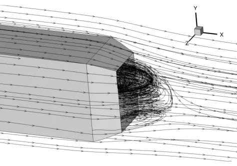
At the base of a tractor-trailer, flow features include massive separation and turbulent shear flow that lower the static pressure and generate significant pressure drag because of the pressure differential between tractor front and trailer base. While base flaps add skin-friction drag and regions of adverse pressure gradient, more significantly they force the trailing wake to shrink, resulting in a region with pressure a little larger than the freestream, which in turn reduces pressure drag [9] and allows for a safer driving environment for vehicles behind or near the tractor trailer. Figure 2 illustrates this with flow visualization from 3-D computational time-averaged solutions at 57.2 mph (92.1 km/h), the average highway speed for tractor trailers in the United States [4], and sideslip angles, β = 9.1° for Figures 2a and 2b, and β = 0° for Figures 2c and 2d. Tractor trailers are subject to random winds on the highway, resulting in different effective sideslip angles seen by the tractor trailer, and these uncertainties are included by considering varied sideslip angles. Figure 2a shows streamlines and gauge pressure (Pgauge = P - P∞, where P∞ is freestream pressure)

contours for the trailer base without flaps, and Figure 2b shows results for the trailer with base flaps; Figures 2c and 2d show stream traces for the two different configurations. Addition of the base flaps visibly reduces the wake size and strength, as indicated by the smaller region of recirculating flow and higher static pressure, resulting in 36% reduction in

̅ . Because the geometry for the computational simulation is simplified and includes forebody rounding, we expect a geometrically complex, full-scale tractor-trailer to experience

roughly half that amount of drag reduction [10, 11]; further, reduction in fuel consumption corresponds to half the reduction in ̅ [2, 8].

(a) Baseline configuration, no flaps, CD = 0.329.

(b) Side flaps deflected inward 20°, CD = 0.201.

(d) Stream traces, all flaps deflected inward 18°.

Figure 2. Time-averaged 3-D computational solutions of full-scale simplified tractor-trailer with and without base flaps, showing reduced region of low pressure. Horizontal slice at y/W = 0.695 for β = 9.1° showing velocity streamlines atop contours of gauge pressure (for (a) and (b)). β = 0° for (c) and (d). Highway speed, V∞ = 57.2 mph (92.1 km/h), and trailer-width-based Reynolds number, ReW = 4.4 x 106_{, reproduced from [4].}

Numerous experimental and some computational studies have been conducted to quantify the drag reduction associated with base flaps. Using various full and scaled-model trucks at various Reynolds numbers (corresponding to typical highway speeds) and with different flap lengths, shapes, and deflection angles, (see [2, 8, 9, 12-15] and summary in [4]), wind-averaged drag reductions ranged from 6 to 19%. However, all of these studies test a relatively small number of design configurations and indicate inconclusive correlations with drag reduction. Freeman and Roy evaluate 130 design configurations and determine an efficient design that maximizes drag reduction by adjusting flap deflection angle (to include holding side flap angles independent of top and bottom flap angles), axial length, and curvature (slope at the leading and trailing flap edges) and that was relatively insensitive to uncertain wind speed and direction, elevation, and mounting accuracy [4]. The present study compares experimental and computational performance estimates of Freeman and Roy’s design with one closely resembling the design of STEMCO Products Inc. that is seen with relative regularity on US highways.

2. Methods

2.1. Experimental Setup

We conduct tests in the US Air Force Institute of Technology (AFIT) open-circuit low-speed wind tunnel. The tunnel test section measures 41 in. (1.041 m) wide by 33 in. (0.838 m) high, including three-sided optical access, and may attain airspeed up to 150 mph (67.1 m/s) or M = 0.2, within the range of incompressible flow. The transverse velocity distribution across the test section and within the boundary layers is typically within 1.0% of the mean, and the turbulence measured at the test section centerline is less than 0.1% at full speed. To measure the axial loads, we use a six-component strain-gauge 10 lbf (44.5 N), force balance. To

ensure accurate measurement of surface static pressure on the model and one tunnel wall, we use ESP pressure scanners with miniature electronic differential pressure measurement using silicon piezoresistive pressure sensors, controlled by Pressure Systems, Inc., digital temperature compensation Initium system. The pressure sensors are rated for pressure ranges from 0 to 30 psi (2.04 atm) and provide static errors within ±0.05% of full-scale pressure range, and the data acquisition system maintains thermal stability within ±0.005% of full-scale pressure range per °C. While wind tunnel solid and wake blockage effects may not be significant for this study because of the limited range of side-slip motion (±14°) and no pitching or rolling motion, we use Barlow et al. to estimate a correction of 0.962 for drag coefficients and 0.974 for pressure coefficients [16].

(a) Drawing showing trailer base flaps device partially in place and pressure tap locations.

(b) Test article in low-speed wind tunnel.

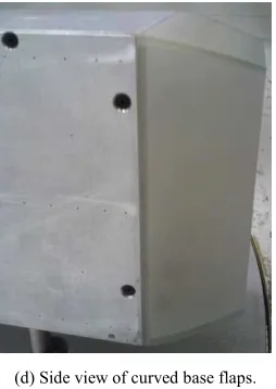
(d) Side view of curved base flaps.

Figure 3. Simplified 1/24-scale model of class-8 cab-over-engine tractor trailer without wheels or cab-trailer gap and with attached rear drag-reduction device.

Figure 3 shows the 1/24 scale model of a class-8 cab-over-engine tractor trailer, simplified by removing all complex geometry, such as grill, side mirrors, exhaust stack, undercarriage, wheels, mud flaps, and cab-trailer gap. In this study, we compare some results with those of Storms et al.,

who use the same model but 1/8 scale in the NASA Ames Research Center 7- by 10-Foot Wind Tunnel #1 [10]. For the model in the present study and shown in Figure 3b, the cab and cab-trailer gap portions are additively manufactured using plastic, and the trailer and bottom portions are machined from ¼-inch aluminum plate. The base drag-reduction devices are also printed with plastic and one is shown in Figures 3c and 3d, where the base device slides over the base using a tongue-and-groove design. Prior to testing, to ensure a smoother physical transition, clear packing tape is applied over the interface between plastic cab and aluminum trailer. The tape is also applied at the interface of trailer and base device to prevent the base device from moving upward during testing.

Figure 4 shows the model that is non-dimensionalized by the trailer width, W, of 4.25 in. (10.80 cm), as well as the 79 pressure taps; a tabular list of the pressure tap locations for the model is included in Appendix 2. The model attachment points are 0.5-in. diameter circular cylinder steel posts and position the model one inch (0.235W) above the tunnel floor. The posts are inside the turbulent boundary layers of the tunnel floor and model underside, and they have no aerodynamic fairings like those used by Storms et al. [10].

Figure 4. Simplified tractor-trailer geometry with pressure tap locations, non-dimensionalized by trailer width, W = 4.25 in. (10.80 cm). Not shown are 3 pressure taps on the starboard side, reproduced from [10].

The mounting posts attach to an air bearing beneath the tunnel floor, such that the displacement in the body axis enables the force measurement. The forward post centerlines are located at 2.428W from the front of the model, and the aft posts are located 4.612W from the forward posts, each post center located 0.118W from the respective lateral edges. Figure 5a shows the location of the model in the test section, noting that the front of the test article is located 4.24W from the front of the tunnel test section. Figure 5b shows the air

(a) Top view of test article on yaw plate, modified from [10]. Dimension at front is not to scale.

(b) Mounting of test article through yaw plate to air bearing and stand on underside of test section.

(d) Test article in tunnel, showing wall pressure taps, tubing, and pressure scanner.

Figure 5. Simplified tractor-trailer model in wind tunnel test section, including mounting setup and wall instrumentation. All measurements are non-dimensionalized by trailer width, W = 4.25 in. (10.80 cm).

2.2. Experiment Accuracy and Uncertainty

The surface pressures on the model and starboard tunnel wall are scanned electronically and time-averaged; they provide an accuracy in pressure measurements of ±0.009 psi (62.1 Pa), and the repeatability of the pressure coefficient measurements is ±0.001 for -6 ≤ β ≤ 6° and ±0.003 for -6 > β > 6°. Following the root-sum-square uncertainty method of Kline and McClintock [17], we estimate the uncertainty in pressure coefficients to be ±0.024, or about 4.8%. The body-axis drag measurements are accurate within ±0.01 lbf (0.044

N), and the repeatability of the drag force coefficient measurements is ±0.003 for -6 ≤ β ≤ 6° and ±0.03 for -6 > β > 6°. These errors include both measurement resolution and point-to-point repeatability. We estimate the uncertainty in drag coefficients to be ±0.032, or about 7.2% for measurements with the tunnel test section inlet flow at 150 mph (67.1 m/s). The largest component in both uncertainty estimates comes from the precision error of the tunnel static pressure port. Only body-axis drag is reported, and no measurements were taken for lift, side force, or moments.

Dynamic pressure, q∞, is measured at the inlet to the

wind tunnel test section, and we record ambient pressure and temperature that are used to calculate the tunnel flow speed. Equation (1) is used to calculate the pressure coefficient,

= (1)

where p is the local measured pressure and p∞ is the reference

pressure (both in psi) obtained when initializing the pressure scanning system at the start of each test run.

From the optimization studies of Freeman and Roy, they determine that the trailer base flaps need to be flush with the base edges for the largest drag reduction. Table 1 lists the

design variables and constraints that are applied to determine an optimal design. None of the constraints are active in the design of interest, meaning the design does not touch the constraint limits. In the current study we evaluate Freeman and Roy’s pseudo-optimal design [4, 18].

Table 1. Trailer base flaps design variables and constraints [4].

Design Variable Description Constraint L1 axial length of trailer base flaps 0.235 ≤ L1/W ≤ 0.471

θ1 slope at flap leading edge 0 ≤ θ1 ≤ 20°

θ2 slope at flap trailing edge -35 ≤ θ2 ≤ 35°

δside side flaps deflection angle 10 ≤ δside ≤ 28°

δtop top/bottom flaps deflection angle 10 ≤ δtop ≤ 28°

Table 2. Trailer base flap test configurations from Freeman and Roy [4] and from STEMCO [12].

Variable Flap Configuration Number

1 2 3 4 5 6 7 8

L1 0 0.42W 0.42W 0.42W 0.47W 0.47W 0.47W 0.42W

θ1 (deg) 0 10 10 10 13 15 17 10

θ2 (deg) 0 20 20 20 13 15 17 20

δsides (deg) 0 17 19 21 13 15 17 19

δtop (deg) 0 14 16 18 13 15 17 16

δbottom (deg) 0 14 16 18 13 15 17 0*

* _{Bottom flap for Configuration 8 has θ1 = θ2 = 0°.}

2.3. Experimental Procedure

To provide more complete validation data for computational modeling, the testing includes running the tunnel without the test article through a variable Mach-number run; with the tractor-trailer model with and without base flaps through static and dynamic runs; and repeating various runs at different times of day to better characterize the effect of temperature on the test data.

For the empty-tunnel Mach sweep, the tunnel initiates at 30 mph (M = 0.04 and ReW = 1x105) and ramps up to 150

mph (M = 0.20 and ReW = 5x105) at increments of 15 mph

(Re = 5x104), with at least 60 seconds of dwell time per Mach number, then ramps back down to 30 mph at the same increments and dwell times.

For the test article with and without the base flaps, we conduct 28 test runs, in addition to the empty-tunnel Mach number run. These runs include two variations of static sideslip angle at constant tunnel velocity, a dynamic sideslip angle run at constant velocity, and static and dynamic Mach number runs at zero sideslip. For the first type of static sideslip angle cases, the tunnel runs at 150 mph with the model at β = 0°, then we rotate the turntable by increments of 2° to β = 14° (nose turning to port), then to β = -14° and back to 0°, with a 60-second dwell time per increment. For the second type of static cases, the tunnel again runs at 150 mph with the model at β = 0°, but in this case, we rotate the turntable to each of six specified sideslip angles, both positive and negative to account for the denser instrumentation being on the port side of the model, and with the same dwell time per angle. The data from these prescribed sideslip angles are then used for wind-averaging the drag coefficient. For the dynamic sideslip angle cases, we rotate the turntable at a rate of 1° every 5 seconds through β = 14° to -14° and back to 0°.

The computational modeling and physical testing account for two uncertain inputs that are included within the design optimization. First, we include the effects of uncertain wind speed and direction, based on the National Oceanic and Atmospheric Administration collection of average monthly wind speed measurements in 250 continental US cities between 1927 and 2002 [19] and on the SAE standard practice for wind-averaging drag coefficients for trucks [6]. Freeman and Roy [18] show that the SAE wind-averaging practice of using weighted CD values from six determined

sideslip angles is sufficiently representative of averaging the

values from a much larger set of angles; thus, the SAE wind-averaging method is an adequate approximation of the more statistically robust method. Second, we include the effects of uncertainty in the base flap deflection angles, where the physical mounting angle may be inaccurate and/or where side winds may create static aeroelastic loading on the flaps and result in off-design deflection angles. We select δ ± 2° for the uncertainty bounds, based on engineering judgment for mounting tolerance and reasonable displacement from wind gusts and based on results from Freeman and Roy’s 2-D investigation [18]. Using the SAE wind-averaging method for freestream velocity, V∞ = 60 mph and average wind speed

of 9.06 mph [18], we obtain β = {2.0, 2.6, 5.5, 6.8, 8.0, 8.6°} and weights, ψ = {1.314, 0.731, 1.236, 0.809, 1.100, 0.945}.

̅ is then calculated according to

̅ = ∑ ( ) (2)

where ( ) = ( )

. (3)

where ρ∞ is freestream density (kg/m3), H is trailer height

(m), and Fx(βi) is the axial force (N) at the respective sideslip

angle, βi, which includes both pressure and skin friction

forces acting over the body surface and base flaps. This force is measured by the strain gauge during tunnel testing and compared with the computational predictions. Further, we can estimate a more robust wind-averaged drag coefficient by taking into account the worst-case result from δ ± 2° at each β; that is, two deflections, zero deflection, and six sideslip angles for a total of 18 drag coefficient values are used to calculate each total wind-averaged drag coefficient.

̅ _{± °= ∑ #$% &' ,) *°}( )+ , ( ), , ,)-*°( )./(4)

2.4. Computational Models

The computational meshes for the Freeman and Roy studies [4, 18] are generated using Gridgen [20] and flow calculations are conducted using the Cobalt computational fluid dynamics (CFD) solver versions 4.2 and 5.2 [21]. For the computational models, we assume a constant V∞ = 57.2

mph (25.6 m/s) for the full-scale optimization study and V∞ =

200 mph (89.4 m/s) for validation with the Storms et al. results, assuming standard temperature, pressure and density (T∞ = 293.15 K, P∞ = 101.325 kPa, ρ∞ = 1.204 kg/m

3

), corresponding to Reynolds number, ReW = 4.4x10

6

0.075 for the full-scale, and ReW = 2.1x106 and M∞ = 0.279

for the Storms et al. validation. For the full-scale study, we use the vehicle geometry of the Sandia National Laboratories Ground Transportation System (GTS) that models a class-8 cab-over-engine tractor trailer and uses the standard length (L = 19.812 m = 65 ft) and width (W = 2.5908 m = 8 ft 6 in.) for US trucks, and a 1/8-scale version for the validation with Storms et al. [10]. The trailer height is modified (H = 3.6068 m = 11 ft 10 in.) to be 28 in. greater than the standard 9 ft 6 in. to represent some of the effects of a trailer skirt and the cab being closer to the ground than the trailer, while the top of the trailer maintains the standard 13 ft 6 in. (4.11 m) above ground [10, 22]. (Note: values for V∞, L, W and H are

assumed to be exact and we neglect the uncertainty associated therewith.) We also choose to remove the wheels for the full-scale study, based on the explanation in [4]; however, for the computational validation study, the model includes the circular mounting posts and wind-tunnel floor, as shown in Figure 6a. Note that surface contours of skin friction coefficient are shown in Figure 6a, but the legend and additional details are not included because this is shown to illustrate the geometry. The full-scale computational domain is shown in Figures 6b, 6c and 6d, and boundary conditions, flow solver parameters, turbulence model selection, solution convergence, grid resolution determination, and estimation of numerical uncertainty are detailed in Freeman and Roy’s studies [4, 18].

(a) Some CFD validation of Storms et al. using Cobalt v4.2, 16x106 _cells,

includes mounting posts and tunnel floor.

(b) Complete computational domain for [4].

(c) Surface geometry and mesh with base flaps.

(d) Base and flaps, horizontal slice at y/W = 0.69.

Figure 6. Computational mesh for simplified 3-D tractor-trailer geometry (GTS model), 5.75x106 _{hexahedral cells, average first-cell y}+ _{≈ 1.3 (for} combined GTS and flaps), where (b), (c) and (d) are reproduced from [4].

3. Results and Discussion

To validate the computational model, we model the 1/8-scale GTS with mounting posts and wind tunnel floor. Using the Cobalt flow solver with Menter shear-stress transport turbulence model and a mesh of 31x106 hexahedral cells, we estimate for β = 0° and no base device attached that =

0.255 ± 0.010. This is 2.0% different from the Storms et al.

measurement of = 0.250 ± 0.01 and within the

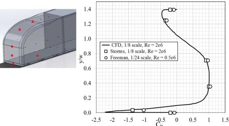
uncertainty band. Furthermore, in Figure 7 we compare CP

measurements from Storms et al. on the front and the base centerlines with our 1/8-scale CFD results at the same ReW. On

the GTS model front centerline in Figure 7a, where the illustration on left indicates the pressure tap locations, CFD (solid line) differs from the Storms experiment (squares) by between 1.0 and 30%, with the larger percentage being where the CP values are close to zero. Our 1/24-scale experiment

results (circles), conducted at ReW = 4.9x105, are also included

and in Figure 7a differ from the Storms experiment by 4 to 60%, with the largest discrepancy occurring at the front near the bottom side, where there is rapid turning and a large acceleration in the local flow. At the trailer base in Figure 7b, differences in the results appear more pronounced because the CP range is smaller; CFD and 1/8-scale experiment differ by 6

to 65%, or ∆CP of 0.02 to 0.12, while the experiments differ by

(a) Surface CP at front of GTS along centerline (z/w = 0); red stars on left show pressure tap locations for data on right, with y/w = 0 at truck underside.

(b) Surface CP at base of GTS along centerline (z/w = 0); red stars on left show pressure tap locations for data on right.

Figure 7. Surface pressure coefficients for GTS model at β = 0° and no base flaps, comparing Storms et al. and CFD, both 1/8-scale at ReW = 2.1x106_{, and} current experiment 1/24-scale at ReW = 4.9x105_.

The baseline computational full-scale model at ReW =

4.4x106 with no flaps predicts ̅ = 0.329- . *7_{. *6}, while Storms et al. at ReW = 2.1x106 measure ̅ = 0.277 ± 0.01

for the no-flaps baseline 1/8-scale model [4, 10]. We may attribute the 18.8% delta to variation in Reynolds number, flow differences between wind tunnel and open road simulated by the CFD, and numerical error from using a relatively coarse mesh. For the current experiment 1/24-scale at ReW = 4.9x105, we measure and calculate ̅ = 0.510 ±

0.036 . With nearly double the wind-averaged drag

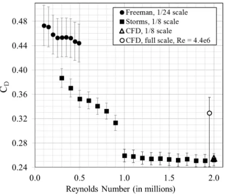
coefficient, we cannot readily attribute the increase to the unfaired mounting posts or different wind tunnel test section shape. In Figure 8, we illustrate the issue of Reynolds-number effects on this geometry. The 1/24-scale drag coefficients (filled circles) for the baseline configuration at

β = 0° for ReW = 0.3, 0.4 and 0.5x10

6

differ from the 1/8-scale values from Storms et al. (squares) by 17, 22 and 26%, respectively, and this delta is more acceptably justified by differences in tunnel and model configurations. Note that the lower uncertainty band for the full-scale CFD result (hollow circle) at ReW = 4.4x10

6

includes the range of data for the 1/8-scale experiment at ReW ≥ 0.9x106. Note also that error

Figure 8. Effect of Reynolds number on drag coefficient for baseline no-flaps configuration at β = 0° for 1/8- and 1/24-scale experiments and full-scale CFD.

After evaluating 130 feasible design candidates and 1,560 flow solutions using CFD, Freeman and Roy determined a design that reduced ̅ more than any other published trailer base-flap design [4]. They do not claim this design is the global minimum because the sampling size is small, so the current study provides further evaluation. Freeman and Roy’s best design, with ̅ _{± °}=0.196- . :_{. 6:}

, shows 40.5% improvement over the wind-averaged no-flaps baseline; for this best design, note that ̅ _0.193

. 7 - .

, which does not include the uncertainty of flap deflection angle, is a 41.5% improvement over the no-flaps baseline. With the 50% cut to drag reduction numbers due to geometry simplification noted in Section II, we might reasonably expect 20-21% reduction in ̅ _{for an actual tractor trailer, which is a vast} improvement over the current best claim of 11% [8], noting again that 20% reduction in drag for a tractor-trailer results in

about 10% reduction in fuel consumption [2, 8]. According to data collected for 2018 by the US Federal Highway Administration, combination trucks (category that includes tractor-trailers but not single-unit trucks) averaged 5.9 miles per gallon (2.5 km/l) and traveled 92.4 billion miles (148.9 billion km) on US rural and urban interstate highways [23]. If we conservatively estimate that 1/3 of that travel would include trailer flaps of our design and based on average US diesel prices for 2018 ($3.18/gal) [24], the 10% reduction in fuel consumption would result in an annual US fuel savings of $1.66 billion and 522 million gallons of diesel; it would also reduce carbon emissions by 10% from the tractor-trailers that use this device.

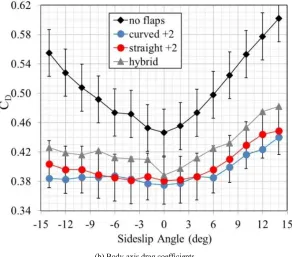
The robustness of our design comes from it accounting for the uncertain effects of wind speed and direction, static aeroelastic loading, mounting inaccuracy, and allowing for different deflection angles on each of the flaps. Figure 9a illustrates this claim by showing that the curved flaps (blue circles) raise the base pressure coefficient (determined at the locations marked with red stars on the left side of Figure 9a) by an average of 83% compared to the baseline (black diamonds), while the straight flaps (red circles) raise it by an average of 70%. An increase in base pressure results in lower pressure drag for the vehicle. Similarly, Figure 9b shows that the δ + 2 configuration for the curved flaps (blue circles) reduces CD from the baseline (black diamonds) by an average

of 22.3%, while the straight flaps (red circles) reduce it by an average of 20.7%; comparison values are similar for the δ - 2 and zero-deflection data. In addition, the slope of the CD

curves in Figure 9b flatten somewhat for the designs with base flaps, indicating less severe flow gradients and greater stability in the base flow. The improvements in both pressure and drag coefficients are more pronounced at the larger yaw angles (β ≥ 6°), confirming that the curved-flaps design is indeed optimized to perform in the uncertain conditions described above.

(b) Body-axis drag coefficients.

Figure 9. Comparison of GTS 1/24-scale model at ReW = 4.9x105 _{with curved flaps, straight flaps, hybrid (configuration 8 in Table 2), and no flaps for -14 ≤ β} ≤ 14°. Asymmetry is shown in the measurements.

We also note in Figures 9a and 9b the asymmetry in pressure and force measurements between the positive and negative yaw angles. For example, we expect in Figure 9a that CP for β = 14° at the starboard base pressure tap would

be approximately equal to the CP value for β = -14° at the

port base pressure tap that is located at the same relative position on the side opposite the starboard tap, assuming the flow, model, and tunnel are even and symmetric about the tunnel vertical centerline. However, the anticipated symmetric values for CP mismatch by between 0.2 and 40%,

where the greater mismatch occurs at the larger yaw angles. This pattern of asymmetry is consistent throughout the data, even with switching the sweep direction; that is, rotating first through negative angles rather than starting with the positive angles. Possible culprits include: (1) a subtle asymmetry in the test article, likely near the front of the GTS model where the influence on the downstream flow would be greatest via the viscous, high-energy boundary layer; or (2) asymmetry in the gap between the yaw plate and tunnel floor, particularly at the larger yaw angles. For option (1), in our early CFD analysis, we detected a laminar separation bubble near the tractor front that is artificially created by small leading-edge breaks in smoothness on the model geometry. Option (2) is more likely, however, since the data at β = 0° collected on opposite sides of the trailer do not manifest the asymmetrical behavior. As a result, for the wind-averaging, we include angles only as large as β = 8.6° where there is smaller departure from symmetrical behavior, and we use results from the positive sweep where the data do not appear to be influenced by the asymmetrical flow behavior.

Freeman and Roy show that their curved-flaps design

̅ _{± °} is 40.5% less than the baseline ̅ , while the

straight-flaps design reduced it by 37.7% [4]. It is further worth noting that a straight-flaps design with an increased deflection of 2° results in ̅ _{± °} that is only 20% smaller than the baseline, which is because flow has separated from the flaps at the perturbed deflection, δ + 2 = 20°; thus, the performance of the straight-flaps competing design is more inclined to diminished performance because of flow behavior sensitivity to the mounted deflection angle. In the current testing, we determined the straight-flaps design yields

̅ _{± °= 0.414 ± 0.029} , or 18.8% reduction from the

baseline no-flaps value, and the curved-flaps design provides

̅ _{± °= 0.407 ± 0.028}, or 20.1% reduction. These results

are summarized in Table 3 and shown graphically in Figure 10. From Figure 10, we observe again that the curved-flaps design out-performs the straight-flaps design at the larger yaw angles, while the straight flaps perform better or the same at smaller angles and zero sideslip. Also, the hybrid design performs worse than the curved- and straight-flaps designs but its ̅ is 14.5% smaller than the baseline. The summarized results in Table 3 and Figure 10 emphasize that our curved-flaps design provides modest but potentially significant improvements over straight or hybrid flaps; careful consideration should be given to the tradeoff between performance and manufacturing complexity and cost. Since the results of this study are neither conclusive nor overwhelmingly convincing due to the Reynolds-number issue and relatively small improvement over the straight flaps, and since we cannot test at a greater ReW in the AFIT

Figure 10. Body-axis, wind-averaged, and total wind-averaged drag coefficients for GTS 1/24-scale model at ReW = 4.9x105 _{with curved flaps, straight flaps,} hybrid, and no flaps for 0 ≤ β ≤ 8.6°.

Table 3. Comparison of GTS base flap designs from Storms et al. [10], current study and Freeman and Roy [4].

Configuration Scale ReW =>_? =>?@±A° =>?improvement over no-flaps

= >

?@±A°improvement over

no-flaps

Storms no flaps 1/8 2.1x106 0.277 ± 0.01 - - -

Parallel 0.225 ± 0.01 - 18.8% -

Freeman

no flaps

1/24 4.9x105

0.510 ± 0.036 - - -

Curved 0.399 ± 0.028 0.407 ± 0.028 21.8% 20.1%

Straight 0.405 ± 0.028 0.414 ± 0.029 20.6% 18.8%

CFD

no flaps

full 4.4x106

0.329- . *7. *6 - - -

Curved 0.193- ._{. 7} 0.196- . :_{. 6:} 41.5% 40.5%

Straight 0.197- ._{. 77} 0.205- . :_{. 67} 40.1% 37.7%

These results show there is greater drag-coefficient sensitivity to ReW below 0.9x106 than to ReW above 2x106,

where the highway speed of 57 mph and a full-scale tractor trailer correspond to ReW = 4.4x106, and accordingly, there

may be greater drag reduction from the curved base flaps that may be validated in an experiment at greater ReW. When we

consider more of the effects on tractor-trailer fuel economy, including aerodynamic (pressure and skin friction) drag, rolling friction, and engine and transmission losses, where travel at greater highway speed requires more power than at lower speeds [25], we find that total drag savings are larger at the lower speed than at the higher highway speed. Thus, greater highway speed results in smaller drag coefficient but not in smaller total drag. The fuel savings result from applying relative increments in drag coefficient reduction that come from base flaps and other devices noted in the introduction.

In Freeman and Roy [4], they discuss model form uncertainty that comes from the lack of experimental

validation of the computational model. The intent of the current study is to reduce or refine that uncertainty through a validation experiment; however, since the AFIT low-speed wind tunnel is limited for this scale to ReW ≤ 4.9x105, unless

we increase the scale of the model along with increased solid and wake blockage errors, a complete validation experiment at the appropriate Reynolds number is not possible in the current facility. Nonetheless, the current study does validate qualitatively and quantitatively the relative improved performance of curved base flaps compared to straight flaps. Further experimental studies and road testing may be merited.

4. Conclusion and Future Work

a simplified 1/24-scale class-8 cab-over-engine tractor-trailer geometry at ReW = 4.9x105.

The Freeman and Roy design is computationally optimized for full-scale highway speed at ReW = 4.4x106 [4], and Storms et al. show that CD remains relatively constant for the GTS model and its devices for 0.9x106 ≤ ReW ≤ 2.1x106 [10]. In our study, we show that CD increases at lower Reynolds numbers, such that this experiment does not fully validate the computationally optimized design. However, the current study does qualitatively and quantitatively validate the relative improved performance of curved base flaps compared to straight flaps. When incorporating the uncertain effects of wind speed and direction and device mounting, the full-scale computational model at ReW = 4.4x106 predicts the curved base flaps reduce ̅ _{± °} by 2.8% more than the straight base flaps, and the current study shows that the 1/24-scale model at ReW = 4.9x105 with curved base flaps reduces ̅ _{± °} by 1.3% more than the straight base flaps. It remains for further study to determine whether this

incremental improvement in drag reduction and fuel consumption is worth the expense of manufacturing a slightly more complex base-flap geometry.

All things considered, we validate that the curved base flaps design performs well in the face of uncertain wind speed and direction and uncertain flap deflection angles, and it has the potential to save billions of dollars in commercial trucking fuel consumption.

Acknowledgements

We express gratitude to Joshua Dewitt and Chris Harkless, both at the Air Force Institute of Technology, for their technical and mechanical expertise. We further acknowledge that some of the wind tunnel test instrumentation was purchased courtesy of a grant from the Air Force Office of Scientific Research.

Appendix

Appendix 1: Nomenclature

CD = body-axis drag coefficient

̅ = wind-averaged body-axis drag coefficient

̅ _{± °} = wind-averaged body-axis drag coefficient that accounts for flap deflection

CP = pressure coefficient

H = trailer height

L = trailer length

M∞ = freestream Mach number

P = local static pressure

P∞ = freestream static pressure

Pgauge = gauge pressure

q∞ = freestream dynamic pressure

ReW = Reynolds number based on trailer width

T∞ = freestream temperature

V∞ = freestream velocity

W = trailer width

Β = side-slip angle

∆ = base flap deflection angle

ρ∞ = freestream density

Ψ = weight factor

Appendix 2: Pressure Tap Locations

References

[1] Mason WT Jr, Beebe PS. The drag related flowfield characteristics of trucks and buses. In: Symposium on aerodynamic drag mechanisms of bluff bodies and road vehicles, General Motors Research Laboratories, Plenum Press, 1978.

[2] Cooper KR. Truck aerodynamics reborn – lessons from the past. SAE technical paper 2003-01-3376, 2003. DOI: 10.4271/2003-01-3376.

[3] Leuschen J, Cooper KR. Full-scale wind tunnel tests of

production and prototype, second-generation aerodynamic drag-reducing devices for tractor-trailers. SAE technical paper 2006-01-3456, 2006. DOI: 10.4271/2006-01-3456.

[4] Freeman JA, Roy CJ. Global optimization under uncertainty and uncertainty quantification applied to tractor-trailer base flaps. ASME J Verification, Validation and Uncertainty Quantification 2016; 1 (2): 021008: 1-16. DOI: 10.1115/1.4033289.

[6] SAE wind tunnel test procedure for trucks and buses. SAE J1252, SAE Recommended Practice, July 1981.

[7] Fuel consumption test procedure – type II. SAE J1321, SAE standard, February 2012.

[8] “Aerodynamics 101,” STEMCO Products Inc., accessed November 14, 2018. http://www.stemco.com/video-gallery

/aerodynamics-101 and

http://www.stemco.com/product/trailertail

[9] Cooper KR. The effect of front-edge rounding and rear-edge shaping on the aerodynamic drag of bluff vehicles in ground proximity. SAE technical paper 850288, February 1985. DOI: 10.4271/850288.

[10] Storms BL, Ross JC, Heineck JT, Walker SM, Driver DM, Zilliac GG. An experimental study of the ground transportation system (GTS) model in the NASA Ames 7- by 10-ft wind tunnel. NASA/TM-2001-209621, February 2001. [11] Lanser WR, Ross JC, Kaufman AE. Aerodynamic

performance of a drag reduction device on a full-scale tractor/trailer. SAE technical paper 912125, September 1991. DOI: 10.4271/912125.

[12] Visser KD, Grover K, Marin LE. Sealed aft cavity drag reducer. US Patent 8,079,634; 2011, accessed June 27, 2012. http://patft.uspto.gov

[13] Browand F, Radovich C, Boivin M. Fuel savings by means of flow attached to the base of a trailer: field test results. SAE technical paper 2005-01-1016, 2005. DOI: 10.4271/2005-01-1016.

[14] Hsu T-Y, Hammache M, Browand F. Base flaps and oscillatory perturbations to decrease base drag. In: McCallen R, Browand F, Ross J (eds.). Lecture notes in applied and computational mechanics, vol. 19: The aerodynamics of heavy vehicles: trucks, buses, and trains, pp. 303-316. Berlin: Springer; 2004.

[15] Ortega JM, Salari K. An experimental study of drag reduction devices for a trailer underbody and base. 34th fluid dynamics conference, AIAA-2004-2252, 2004.

[16] Barlow JB, Rae WH Jr, Pope A. Low-speed wind tunnel testing, 3d Edition. New York: Jon Wiley & Sons; 1999.

[17] Kline JS, McClintock FA. Describing uncertainties in single-sample experiments. ASME J Mech Eng, 1953, 1: 3-8.

[18] Freeman JA, Roy CJ. Application of optimization under uncertainty: 2-d tractor-trailer base flaps. AIAA-2012-0671, 2012.

[19] Dellinger D. Average wind speed. National Oceanic and Atmospheric Administration, 2008, accessed June 19, 2012.

http://lwf.ncdc.noaa.gov/oa/climate/online/ccd/avgwind. html

[20] Gridgen version 15 user manual. Pointwise, Inc., Texas, 2006. [21] Cobalt version 5.2 user’s manual. Cobalt Solutions,

LLC., Ohio, 2011.

[22] Gutierrez WT, Hassan B, Croll RH, Rutledge WH. Aerodynamics overview of the ground transportation systems (GTS) project for heavy vehicle drag reduction. SAE Technical Paper 960906, February 1996. DOI: 10.4271/960906.

[23] “Annual vehicle distance traveled in miles and related data by highway category and vehicle type,” 2016, Table VM-1, Highway Statistics, Office of Highway Patrol Information, Federal Highway Administration, US Department of Transportation, accessed November 14, 2018. https://www.fhwa.dot.gov/policyinformation/

statistics/2016/vm1.cfm.

[24] “US on-highway diesel fuel prices,” 2018, US Energy Information Administration, accessed November 14, 2018. https://www.eia.gov/petroleum/gasdiesel