An Explicit Expression of Average Run Length of Exponentially Weighted Moving Average Control Chart with ARIMA (p,d,q)(P, D, Q)L Models

Article

An Explicit Expression of Average Run Length of

Exponentially Weighted Moving Average Control

Chart with ARIMA (p,d,q)(P, D, Q)

L

Models

Yupaporn Areepong * and Saowanit Sukparungsee

Department of Applied Statistics, Faculty of Applied Science, King Mongkut’s University of Technology North Bangkok, 1518 Pracharat 1 road, Wongsawang, Bangsue, Bangkok 10800, Thailand ;

[email protected]

* Correspondence: [email protected]; Tel.: +66-2-555-2000

Abstract: In this paper we propose the explicit formulas of Average Run Length (ARL) of Exponentially Weighted Moving Average (EWMA) control chart for Autoregressive Integrated Moving Average: ARIMA(p,d,q) (P, D, Q)L process with exponential white noise. To check the accuracy, the ARL results were compared with numerical integral equations based on the Gauss-Legendre rule. There was an excellent agreement between the explicit formulas and the numerical solutions. Additionally, we compared the computational time between our explicit formulas for the ARL with the one obtained via Gauss-Legendre numerical scheme. The computational time for the explicit formulas was approximately one second that is much less than the numerical approximations. The explicit analytical formulas for evaluating ARL0 and ARL1 can produce a set of optimal parameters which depend on the smoothing parameter (_λ) and the width of control limit (H), for designing an EWMA chart with a minimum ARL1.

Keywords: exponentially weighted moving average control chart (EWMA); autoregressive integrated moving average (ARIMA); average run length (ARL)

1. Introduction

tighter than desired. It has been observed that the main effect of autocorrelation in process data for a traditional chart is that the Average Run Length of the in-control processes may be shorter than intended. Processes with serially correlated data need to be monitored by appropriate control charts. Two measures that are commonly used to compare the performance of control charts are the Average Run Length for in control process (ARL0) and the Average Run Length for out of control process (ARL1). The ARL0 is the average number of observations that will occur before an in-control process falsely gives an out-of-control signal. To reduce the number of false out-of-control signals a sufficiently large ARL0 is required. The ARL1 is a measure of the average number of observations that will occur before an out-of-control process correctly gives an out-of-control signal. To reduce the time that the process is out-of-control, a small ARL1 is required. Therefore the ARL and ARL1 are two conflicting criteria that must be balanced to give an optimal control chart.

Three standard methods that are often used to evaluate Average Run Length for in control process (ARL0) and the Average Run Length for out of control process (ARL1) are the Markov Chain Approach (MCA), the Integral Equation (IE) and the Monte Carlo simulation (MC) methods. Roberts [3] evaluated the ARL for EWMA control charts using the MC technique. Crowder [4] computed the ARL of an EWMA chart from numerical solutions to an integral for Gaussian observation. Lucas and Saccucci [1] employed a finite state Markov chain approximation to develop tables to assist users of EWMA control charts in these choices.

The methods used for the evaluation of the characteristics of EWMA control charts for serial correlated data were studied. Mastrangelo and Montgomery [7] have been evaluated the performance of EWMA control charts for serially-correlated observation using Monte Carlo simulation technique. Vanbrackle and Reynold [8] studied EWMA and CUSUMcontrol charts by using an Integral Equation and Markov Chain Approach to evaluate the ARL in case of AR(1) process with additional random error. Harris and Ross [9] discussed the effect of autocorrelation on the performance of EWMA and CUSUM charts. They found that the Average Run Lengths and Median Run Lengths of these charts were sensitive to autocorrelation. Later, Reynolds and Lu [10] studied the EWMA control charts using simulation based on the observations from the AR(1) process plus a random error of detecting change in the process mean or variance. Lu and Reynolds [11] presented the ARL of the EWMA control chart based on residual from the forecast value for monitoring the mean of the process for an AR(1) process plus a random error using an integral equation method. Apley and Lee [12] presented a technique for designing residual based EWMA charts under conditions of model uncertainty. Shiau and Chen [13] investigated the robustness of modified individual Shewhart and modified exponentially weighted moving average (EWMA) charts for normality assumption of the white noise term for AR(1) process with positive autocorrelation. Rosolowski and Schmid [14] measured ARL of EWMA charts by monitoring the mean of the stationary processes with heavy tailed distribution using simulation. Mititelu et al. [15] presented explicit formulas for the ARL of EWMA and CUSUM charts when the observations have a hyper exponential distribution, using the Fredholm integral equations approach. Recently, Suriyakat et al. [16] derived an exact solutions of ARL for EWMA control charts for AR(1) process observations with exponential white noise. Busaba et al. [17] have studied an explicit formula of ARL for cumulative sum charts using negative exponential data. Petcharat et al. [18] presented closed form expression of the ARL for CUSUM chart for MA(1) processes with exponential white noise using integral equations. Phanyaem et al. [19] presented Explicit formulas of average run length for ARMA(1,1) using the Fredholm integral equations approach.

In this research the objective is to derive explicit formulas for detecting changes in the mean of the process of EWMA control charts for ARIMA(p,d,q) (P,D,Q)LProcess with exponential white noise. Additionally, the explicit formulas of ARL0 and ARL1 can be able to generate a set of optimal parameters which depend on the smoothing parameter (

λ

) and the width of control limit control limit (

H

) for designing EWMA charts with a minimum of ARL1.

Let

ξ ξ

₁

, ,...,

₂ be sequentially observed independent random variables with a distribution

( )

,

β

F x

where

β

is a parameter. We study the change-point detection problem, i.e. of detecting

if and when the value of the parameter

β

changes. The change-point model for the exponential distribution may be stated as follows. We assume that:

0

1

( ),

1, 2,...,

1

,

( ),

,

1,

2,...

t

Exp

t

Exp

t

β

θ

ξ

β

θ θ

θ

=

−





=

+

+





where

β

₀and

β

₁are known parameters. Usually, the parameter value

β

₀is assumed to

define the in-control state and the parameter value

β

₁ to denote an out-of-control state. We assume

that the value

β

₀is maintained up to some unknown time

θ

−

1

_{and that at time}

θ

the parameter value changes to the new value

β β

>

₀. The time

θ

is called "the change-point time".

The typical condition of choice of the stopping times

τ

is as follows:

,

)

(

T

E

∞

τ

=

where T is given (usually large), and

E

_∞

(.)

denotes that the expectation under distribution

0

( ,

β

)

F x

, ‘in-control’ is that the change-point occurs at point

θ

(where

θ

≤ ∞

). In the literature

on quality control, the quantity

E

_∞

( )

τ

is called the Average Run Length for ‘in-control’ processes

(ARL0). Then, by definition,

ARL

₀

=

E

_∞

( )

τ

and the typical practical constraint is:

0= ∞( )

τ

= .

ARL E T (1)

Another common constraint consists of minimizing the quantity:

(

)

1

1

,

ARL

=

E

_θ

τ θ

− +

τ θ

≥

(2)

where

E

_θ

(.)

is the expectation under distribution,

F x

( , )

β

1 ‘out-of-control’ and

β

is the value

of the parameter after the change-point. There is restriction on the special case, usually

θ

=

1

. The quantity

E

₁

( )

τ

is called the Average Run Length for ‘out-of-control’ processes (ARL1) and it could be expected that a sequential chart would have a near optimal performance if ARL1 is close to minimal value.

The definition of EWMA statistics based on ARIMA(p,d,q)(P, D,Q)Lprocess is the following recursion:

1

(1 ) 1,2,....,

t t t

Z = −

λ

Z− +

λ

X ; t = (3)

where Z_t is the EWMA statistic, X_t is a sequence of ARIMA(p,d,q)(P,D, Q)L process,

λ

is a smoothing parameter, and the initial value is a constant (Z₀ = u).

The general autoregressive processes denoted by ARIMA (p,d,q)(P, D, Q)L process can be written as:

d L D 2 P L 2L PL

1 2 P L 2L PL t

(1 B) (1 B ) (1

−

−

− φ − φ

B

B

− − φ

...

B )(1

− φ

B

− φ

B

− − φ

...

B )X

2 q L 2L qL

0

(1

1

B

2

B

...

q

B )(1

L

B

2L

B

...

qL

B ) ,

t

θ + − θ − θ

− − θ

− θ

− θ

− − θ

ξ

(4)

where

ξt

are independent and identically distributed observed sequences of Exponential

average coefficient

− ≤ ≤

1

θ

_i

1

, a seasonal autoregressive coefficient

− ≤

1

φ

_iL

≤

1

and a seasonal moving average coefficient

− ≤

1

θ

_iL

≤

1

. It is assumed the initial value of ARIMA(p,d,q)(P,D,Q)L process equal to 1.

The first passage time of an EWMA chart is denoted by:

inf{

0 :

}

H

t

Z

t

H

τ

=

≥

≥

, (5)

where

H

is constant parameter known as the upper control limit.

3. ARL Explicit Formulas for ARIMA(p,d,q)(P,D,Q)LProcess of EWMA Chart

In this section, we derive explicit solution of Fredholm Integral Equation of the second kind

which is called ARL explicit formulas of EWMA chart for ARIMA(p,d,q)(P,D,Q)Lprocess. Let

L u

( )

denote the ARL of a one-sided EWMA control chart when the initial value is

u

,

0= .

Z u Since

ξ

_t

≥

0

we can assume that the lower and upper limits are H_L =0 and

H

_U

=

H

respectively. For the EWMA statistics Z₁ in an in-control state:

1

0 (1< −λ)Zt− +λXt <H.

Then the function L u( ) is defined as follows:

0

( )= _∞

( )

τ

≥

,

=

.

L u



T Z

u

(6)

To consider the functionL u( ):

1 1 ₁

( ) 1 ( ) ( ) .

L u = +



L Z f ξ ξd (7)

Equation 7 is a Fredholm integral equation of the second kind. Consequently the function L u( ) is obtained as:

( ) 1 ((1 ) t) ( ) . L u = +



L −λu+λX f y dy

Changing the integration variable, the function L u( ) is given by:

0

1 (1 ) ( ) 1 H ( ) ( t)

y u

L u L y f λ X dy

λ λ

− −

= +  − ₍₈₎

Therefore, we obtain

(1 )

0

1

( ) ( ) .

t

X u y H

L u L y e e dy

λ λβ β λβ

λβ

 − ₊ 

−  

 



=

Let the function G u( ) be given by:

(1 )

( ) .

t X u

G u e

λ λβ β

 − ₊ 

 

 

=

Consequently,

0

( )

( ) 1 ( ) ; 0 .

y H

G u

L u L y e λβdy u H

λβ

−

= +



≤ ≤

Let 0

( ) ,

y H

k=



L y e−λβdy

so we have; L u( ) 1 G u( )k.

λβ

= +

(1 )

1 ( ) 1

t

X u

L u e k

λ λβ β λβ  − ₊     

= + (9)

Solving a constant k;

( )( 1) _.

1

1 ( 1)

t H X H e k e e λβ β β λβ λ −   −     − − = + −

Substituting k into Eq. (9) thus the function

L u

( )

can be written as

(1 )

( 1)

( ) 1 .

1

1 ( 1)

t t X u H X H e e L u e e λ λβ β λβ β β λ  − ₊  ₋       −     − = − + − (10)

As mentioned above, the value of the parameter β is equal to β₀ when the process is in

control process. Therefore, substituting β β= 0 into Eq. (10) gives the formula for the ARL0 as:

0 0 0

0 0

(1 )

0 1 ( 1).

1

1 ( 1)

t t X u H X H e e ARL e e λ λβ β λβ β β λ  − ₊  −       −     − = − + − (11)

The formula for ARL1 can be obtained in a similar manner. When the process is out of control process the value of the parameter β in Eq. (11) will be β β= 1. The formula for ARL1 can therefore

be written as:

1 1 1

1 1 (1 ) 1 ( 1) 1 , 1

1 ( 1)

t t X u H X H e e ARL e e λ λβ β λβ β β λ  − ₊  −       −     − = − + − (12)

where X_t is a sequence of ARIMA(p,d,q)(P,D,Q)Lprocess,

λ

∈(0,1) is the smoothing parameter,

u

is the initial values and H is the upper control limit.

According to Equation 11 and 12, for example, the explicit formulas of ARL, for example ARIMA(1,1,1)(0,1,1)L process can be written

X

_t as

1 1 1 (1 ) 1 (1 ) 1 1 1 (1 ) 1 2 1 (2 )

t t t L t L L t L t L t t L t t L t t L

X = +μ ξ −θ ξ₋ −θ ξ₋ +θ θ ξ_{− +} +X₋ +X₋ −X_{− +} +φX₋ −φX_{− +} −φX₋ +φX_{− +}

ARIMA(0,1,2)(1,1,2)L process can be written

X

_t as

1 1 2 2 1 2 2 (2 ) 2 2 1 2 (1 2 L)

1 (1 ) 2 (1 ) (1 2 )

t t t t L t L t L L t L L t L L t

t L t t L L t L L t L L t L L t L

X

X X X X X X X

μ ξ θ ξ θ ξ θ ξ θ θ ξ θ θ ξ θ ξ θ θ ξ φ φ φ φ − − − + − + − − + − − − + − − − + − + = + − − − + + − + + + − + − − +

ARIMA(0,1,1)(1,0,2)L process can be written

X

_t as

1 1 1 (1 ) 2 2 1 2 (1 2L) 1 (1 )

t t t L t L L t L L t L L t t L t L L t L

X = +μ ξ −θ ξ₋ −θ ξ₋ +θ θ ξ_{− +} −θ ξ₋ +θ θ ξ_{− +} +X₋ +φ X₋ −φ X_{− +}

Using the explicit formulas in Equation 11 and 12, we can provide the tables for the optimal smoothing parameter (

λ

) and width of control limit (

H

) for designing EWMA chart with minimum of ARL1. We firstly describe a procedure for obtaining optimal designs for EWMA chart. The criterions for choosing optimal values are smoothing parameter (

λ

) and width of control limit (

H

) for designing EWMA chart with minimum of ARL1 for a given in-control parameter value

0

(λ,H) values for T= 370 and magnitudes of change. Table of the optimal parameters values are shown in Table 4.

The numerical procedure for obtaining optimal parameters for EWMA designs

1. To select an acceptable in-control value of ARL and decide on the change parameter value (β₁) for an out-of-control process.

2. For given β₀and T, find optimal values of

λ

and H to minimize the ARL1 (ARL1*) values given by equation 12 subject to the constraint that ARL0=T in Equation 11, i.e.

λ

and H are solutions of the optimality problem

4. Numerical Results

In this section, we compare the results of ARL0 and ARL1 for ARIMA(p,d,q)(P,D,Q)Lprocess which obtained from the explicit formulas with numerical solution of integral equation method for the number of division point m = 500. A numerical scheme to evaluate solution of the integral equations (IE) is given by

1

1

( ) = 1

( ) (

_t

)

m _j

(

_j

) (

_{j t}

).

j

L u

L a F a u X

w L a

f a

a u X

=

+

− −

+



+ − −







₍₁₃₎

where

(

1

)

2

j

H

a

j

m

=

−

and

w

_j

=

H

m

;

j

= 1, 2,..., .

m

The results of ARL are presented in Table 1 - Table 3. The parameter values for EWMA chart were chosen by given desired ARL0 = 370 and 500, in-control parameter β₀= 1 and magnitudes of change. We consider the performance of the explicit formulas in term of the computational times and the absolute percentage difference can be computed as follows:

( )

%

Explicit Formulas Numerical IE

100.

Explicit Formulas

ARL

ARL

Diff

ARL

−

=

×

We compare the numerical results for ARL0 and ARL1 for Exponential (1) obtained from explicit formulas with results obtained from the Integral Equation method for parameter values

λ

=

0.05

. The table shows that the outputs obtained by explicit formulas are very close to IE results. The choice of method for calculating ARL values should therefore be made based on other factors (e.g. CPU times, available software or programming). However, the table also shows that the computational time for evaluating the suggested formula is much less than the CPU times required for IE method. The numerical results in terms of optimal EWMA smoothing parameter (

λ

) and width of control limit (

H

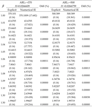
) and minimal of ARL1 are shown in Table 4. For example, if we want to detect a parameter change from β₀=1 to β₁=1.05 and the ARL value is T = 370, then the optimality procedure given

Table 1. Comparison of ARL values for ARIMA (1,1,1)(0,1,1)12 using explicit formula against NIE

whenλ=0.05

φ

₁

=

0.2,

θ

₁

=

0.2,

θ

₁₂

=

0.2

β

ARL

0 =370

H=0.0266609 Diff (%)

ARL0 =500

H=0.0266759 Diff (%) Explicit Numerical IE Explicit Numerical IE

.

1 00 370.101

(0.14) 370.1009 (17.682) 0.00003

500.589 (0.14)

500.589

(18.361) 0.00000

1.01 43.6705 (0.14)

43.6705

(17.821) 0.00000

45.0132 (0.14)

45.0132

(18.429) 0.00000

1.02 23.6665 (0.14)

23.6665

(18.116) 0.00000 24.0439

(0.14)

24.0439

(18.617) 0.00000

1.03 16.4421 (0.14)

16.4421

(18.372) 0.00000

16.6181 (0.14)

16.6181

(19.015) 0.00000

1.04 12.7154 (0.14)

12.7154

(17.757) 0.00000 12.8175

(0.14)

12.8175

(18.447) 0.00000

1.05 10.4413 (0.14)

10.4413

(18.522) 0.00000

10.5082 (0.14)

10.5082

(18.603) 0.00000

1.06 8.90899 (0.14)

8.90898

(17.734) 0.00011

8.95634 (0.14)

8.95633

(18.738) 0.00011

1.07 7.8063 (0.14)

7.8063

(18.142) 0.00000 7.84171

(0.14)

7.8417

(18.862) 0.00013

1.08 6.97476 (0.14)

6.97476

(18.469) 0.00000

7.0023 (0.14)

7.0023

(19.026) 0.00000

1.09 6.32527 (0.14)

6.32527

(18.718) 0.00000 6.34736

(0.14)

6.34736

(18.761) 0.00000

1.10 5.80392 (0.14)

5.80392

(17.972) 0.00000

5.82207 (0.14)

5.82207

(19.152) 0.00000

1.30 2.63948 (0.14)

2.63948

(18.438) 0.00000

2.64204 (0.14)

2.64203

(19.384) 0.00038

1.50 1.99607 (0.14)

1.99607

(19.216) 0.00000

1.99719 (0.14)

1.99719

(19.493) 0.00000

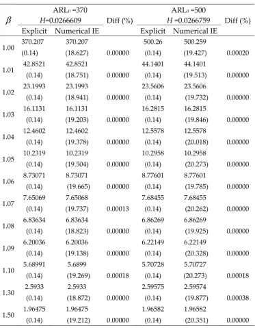
Table 2. Comparison of ARL values for ARIMA (0,1,2)(1,1,2)6 using explicit formula against NIE

whenλ=0.05

φ

₆

=

0 1

. ,

θ

₁

=

0 1

. ,

θ

₂

=

0 1

. ,

θ

₆

=

0 1

. ,

θ

₁₂

=

0 1

.

β

ARL

0 =370

H=0.0266609 Diff (%)

ARL0 =500

H=0.0266759 Diff (%) Explicit Numerical IE Explicit Numerical IE

.

1 00 370.207 (0.14)

370.207

(18.627) 0.00000 500.26

(0.14)

500.259

(19.427) 0.00020

1.01 42.8521 (0.14)

42.8521

(18.751) 0.00000 44.1401

(0.14)

44.1401

(19.513) 0.00000

1.02 23.1993 (0.14)

23.1993

(18.941) 0.00000 23.5606

(0.14)

23.5606

(19.732) 0.00000

1.03 16.1131 (0.14)

16.1131

(19.203) 0.00000 16.2815

(0.14)

16.2815

(19.846) 0.00000

1.04 12.4602 (0.14)

12.4602

(19.378) 0.00000 12.5578

(0.14)

12.5578

(20.018) 0.00000

1.05 10.2319 (0.14)

10.2319

(19.504) 0.00000 10.2958

(0.14)

10.2958

(20.273) 0.00000

1.06 8.73071 (0.14)

8.73071

(19.665) 0.00000

8.77601 (0.14)

8.77601

(19.785) 0.00000

1.07 7.65069 (0.14)

7.65068

(19.737) 0.00013 7.68455

(0.14)

7.68455

(20.262) 0.00000

1.08 6.83634 (0.14)

6.83634

(18.823) 0.00000 6.86269

(0.14)

6.86269

(19.925) 0.00000

1.09 6.20036 (0.14)

6.20036

(19.138) 0.00000 6.22149

(0.14)

6.22149

(20.328) 0.00000

1.10 5.68991 (0.14)

5.6899

(19.269) 0.00018

5.70728

(0.14)

5.70727

(20.273) 0.00018

1.30 2.5933 (0.14)

2.5933

(18.872) 0.00000

2.59575

(0.14)

2.59574

(19.877) 0.00038

1.50 1.96475 (0.14)

1.96475

(19.212) 0.00000

1.96582

(0.14)

1.96582

(20.351) 0.00000

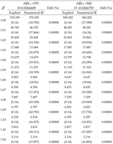
Table 3. Comparison of ARL values for ARIMA (0,1,1)(1,0,2)4 using explicit formula against NIE

whenλ=0.05

θ

₁

=

0.1,

θ

₄

=

0.2,

θ

₈

=

0.3

β

ARL

0 =370

H=0.0266609 Diff (%)

ARL0 =500

H=0.0266759 Diff (%) Explicit Numerical IE Explicit Numerical IE

.

1 00 370.359 (0.14)

370.359

(18.783) 0.00000 500.202

(0.14)

500.202

(17.588) 0.00000

1.01 46.745 (0.14)

46.745

(17.466) 0.00000 48.281

(0.14)

48.281

(16.24) 0.00000

1.02 25.428 (0.14)

25.428

(14.196) 0.00000 25.863

(0.14)

25.863

(18.954) 0.00000

1.03 17.684 (0.14)

17.684

(16.879) 0.00000 17.887

(0.14)

17.887

(18.606) 0.00000

1.04 13.679 (0.14)

13.679

(19.531) 0.00000 13.797

(0.14)

13.798

(18.289) 0.00000

1.05 11.233 (0.14)

11.233

(18.199) 0.00000 11.310

(0.14)

11.310

(16.941) 0.00000

1.06 9.583 (0.14)

9.583

(18.82) 0.00000 9.637 (0.14)

9.637

(19.64) 0.00000

1.07 8.394 (0.14)

8.394

(17.472) 0.00000 8.435 (0.14)

8.435

(19.385) 0.00000

1.08 7.497 (0.14)

7.497

(18.108) 0.00000 7.529 (0.14)

7.529

(19.069) 0.00000

1.09 6.797 (0.14)

6.797

(62.792) 0.00000 6.823

(0.14)

6.823

(17.736) 0.00000

1.10 6.234 (0.14)

6.234

(16.475) 0.00000 6.255

(0.14)

6.255

(18.451) 0.00000

1.30 2.814 (0.14)

2.814

(18.111) 0.00000 2.817

(0.14)

2.817

(17.087) 0.00000

1.50 2.114 (0.14)

2.114

(17.857) 0.00000 2.116

(0.14)

2.116

(16.802) 0.00000

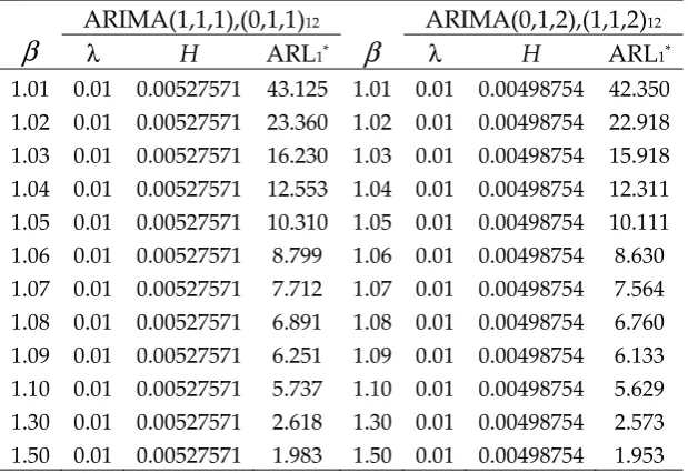
Table 4. Optimal design parameters and ARL1* for EWMA chart given

β

₀=1, ARL0 =370.

β

ARIMA(1,1,1),(0,1,1) 12

β

ARIMA(0,1,2),(1,1,2) 12

λ H ARL1* λ H ARL1*

1.01 0.01 0.00527571 43.125 1.01 0.01 0.00498754 42.350 1.02 0.01 0.00527571 23.360 1.02 0.01 0.00498754 22.918 1.03 0.01 0.00527571 16.230 1.03 0.01 0.00498754 15.918 1.04 0.01 0.00527571 12.553 1.04 0.01 0.00498754 12.311 1.05 0.01 0.00527571 10.310 1.05 0.01 0.00498754 10.111 1.06 0.01 0.00527571 8.799 1.06 0.01 0.00498754 8.630 1.07 0.01 0.00527571 7.712 1.07 0.01 0.00498754 7.564 1.08 0.01 0.00527571 6.891 1.08 0.01 0.00498754 6.760 1.09 0.01 0.00527571 6.251 1.09 0.01 0.00498754 6.133 1.10 0.01 0.00527571 5.737 1.10 0.01 0.00498754 5.629 1.30 0.01 0.00527571 2.618 1.30 0.01 0.00498754 2.573 1.50 0.01 0.00527571 1.983 1.50 0.01 0.00498754 1.953

5. Conclusions

We have presented the explicit formulas for Average Run Length of EWMA chart for Autoregressive Integrated Moving Average: ARIMA (p,d,q)(P, D, Q)L process for the case of an exponential white noise. We have shown that the proposed explicit formulas are easy to calculate and program. The explicit formulas obviously take the computational time much less than Numerical Integral Equation method.

Acknowledgments: The authors would like to express my gratitude to King Mongkut’ s University of

Technology North Bangkok and the Office of the Higher Education Commission, Thailand for supporting

research grant No: KMUTNB-GOV-59-17.

References

1. Lucas, J.M.; Saccucci, M.S. Exponentially weighted moving average control schemes: properties and enhancements. Technometrics1990, 32, 1-29.

2. Srivastava, M.S.; Wu, Y. Evaluation of optimum weights and average run lengths in EWMA control schemes. Communications in Statistics: Theory and Methods, 1997, 26, 1253-1267.

3. Roberts, S.W. Control chart tests based on geometric moving average. Technometrics1959, 1, 239-250. 4. Crowder, S.V. A simple method for studying run length distributions of exponentially weightedmoving

average charts. Technometrics1987,29, 401-407.

5. Yashchin, E. Some aspects of the theory of statistical control schemes. IBM Journal of Research and Development 1987, 31, 199-205.

6. Ye, N.; Borror, C.; Zhang,Y. EWMA techniques for computer intrusion detection through anomalous changes in event intensity. Quality and Reliability Engineering International2002, 18, 443-451.

7. Mastrangelo, C.M.; Montgomery, C.M. SPC with correlated observations for the chemical and process industries. Quality and Reliability Engineering International1995, 11, 79-89.

8. VanBrackle, L.; Reynolds, M.R. EWMA and CUSUM control charts in the presence of correlation. Communications in Statistics-Simulation and Computation 1997, 26, 979-1008.

9. Harris, T.J.; Ross, W.H. Statistical process control procedures for correlated observations. The Canadian Journal of Chemical Engineering1991, 69, 48-57.

10. Reynolds, R M.R.; Lu, C.W. Control chart for monitoring processes with autocorrelated data. Nonlinear Analysis, Theory, Methods & Applications, 1997, 30, 4059- 4067.

12. Apley, D.W.; Lee, H.C. Design of Exponentially Weighted Moving Average Control chairs for autocorrelated process with model uncertainity. Technometrics2003, 45, 187-198.

13. Shiau, J.J.H.; Chen, Y.H. Robustness of the EWMA control chart to Non-normality for Autocorrelated process. Quality Technology & Quantitative Management2005, 2, 125-146.

14. Rosołowski, M.; Schmid, W. EWMA charts for monitoring the mean and the autocovariance of stationary processes. Statistical Papers 2006, 47, 595-630.

15. Mititelu, G.; Areepong,Y.; Sukparungsee, S.; Novikov, A.A. Explicit analytical solutions for the average run length of CUSUM and EWMA chart. Contribution in Mathematics and Applications

II

East-West Journal of Mathematics special volume2010, 253-265.

16. suriyakat, W.; Areepong, Y.; Sukparungsee, S.; Mititelu, G. On EWMA procedure for AR(1) observations with Exponential white noise. International Journal of Pure and Applied Mathematics 2012, 77, 73-83.

17. Busaba, J.; Sukparungsee, S.; Areepong, Y.; Mititelu, G. Numerical Approximations of Average Run Length for AR(1) on Exponential CUSUM. In proceeding of the International MutiConference of Engineers and Computer Scientists, Hong Kong, 2012, 14- 16 March.

18. Petcharat, K.; Areepong, Y.; Sukparungsee, S.; Mititelu, G. Exact solution of average run length of EWMA chart for MA(q) processes. Far EastJournal of Mathematical Sciences 2013, 78, 291-300.

19. Phanyaem, S.; Areepong, Y.; Sukparungsee, S.; Mittitelu, G. Explicit formulas of average run length for ARMA(1,1). International Journal of Applied Mathematics and Statistics2013, 43, 392-405.