Realization of Maxwell’s Hypothesis
(Ⅰ)
A Heat-Electric Conversion in Contradiction to the Kelvin Statement
Xinyong Fu & Zitao Fu Shanghai Jiao Tong University [email protected] May 21, 2019
Key Words
Maxwell’s demon magnetic demon entropy reducing energy circulation
Abstract
In a vacuum tube, two identical and parallel Ag-O-Cs surfaces, A and B, with a work function of 0.8eV, ceaselessly emit thermal electrons at room temperature. The thermal electrons are controlled by a static uniform magnetic field (a magnetic demon), and the number of electrons migrate from A to B exceeds the one from B to A, (or vice versa). The net migration from A to B quickly results in a charge distribution: A charged positively and B negatively. A potential difference between A and B emerges, and the tube outputs ceaselessly an electric current and a power to a resistance (a load) and cools itself slightly. The ambient air is a single heat reservoir in the experiment, and all the heat extracted by the tube from the air is converted into electric energy without producing other effect. We believe the experiment is in contradiction to the Kelvin statement of the second law.
Experiment Video
We have a clear video on YouTube showing the main measuring process of the experiment, about 30 minutes: https://www.youtube.com/watch?v=PyrtC2nQ_UU.
1. Fundamental Concept
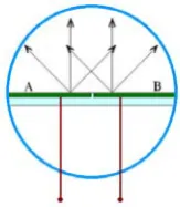
Let us first imagine an ideal vacuum tube containing a quartz plate, as shown in Fig 1.
The upper surface of the quartz plate is coated with two identical and parallel Ag-O-Cs
electron emitters, A and B. The work function of Ag-O-Cs is only 0.8eV, hence, A and
B eject thermal electrons ceaselessly at room temperature (the well known “dark
current” in a phototube or a photomultiplier.)
Fig.2 (a) illustrates the motion of the thermal electrons emitted from two symmetric
points on A and B when no magnetic field is applied to the tube. The thermal electrons
exit from A or B, fly straight forward, hit the glass wall and bounce back, and finally
fall down into the emitters. There are electrons migrate from A to B and from B to A (A
and B like two islands). Statistically, the number of electron migration from A to B and
the one from B to A cancel each other. There is no net electron migration between A and
B, hence, no current outputs to the exterior resistor. (1)(2)
Fig 2 Thermal electrons’ motion with or without a magnetic field
Now, if a static uniform magnetic field is applied to the electron tube in the direction
parallel to the tube axis (the Z-axis), and, firstly, directed into the plane of the figure, as
shown in Fig 2(b), all the thermal electrons will fly clockwise along circles (in the XOY
plane) of different radii according to their speeds,
v
eB
m
R
=
where v is the velocity component perpendicular to the Z-axis.
We omit the discussion about the thermal electron’s Z-component motion.
At t = 20oC for example, the most probable speed of the thermal electrons is vp =
94.3km/s. If we choose the magnetic induction intensity of the field to be B = 1.34 ×
10-4
tesla = 1.34 gauss, the corresponding radius of the thermal electrons of v= vp =
94.3km/s is R = 4mm (more exactly, 4.002mm). For electrons of v = 0.5vp, the
corresponding radius is R = 2mm. For electrons of v= 2vp, the corresponding radius is
The diameter of the glass tube is 28mm.
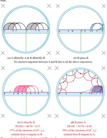
There are numerous and various electron trajectories, of different exiting angles,
different speeds, and different exiting spots. Thermal electrons emitted from A may fall
back to A, or migrate to B. Thermal electrons emitted from B may fall back to B, or
migrate to A. All the trajectories may thus be divided into four groups(3).
(1) The first group: A-A = A-directly-A + A-glass-A
A-directly-A Part of the electrons emitted from A directly (without collision with the
glass wall) fall back to A. Examples, the left part of Fig 3(a), from E to P, M to O, etc.,
grey.
A-glass-A Part of the electrons emitted from A hit the glass wall and bounce back to
A. Examples, absent in Fig 3, appear for some electrons of other exiting angles or
speeds.
All the trajectories of the first group result in no electron migration between A and B, and they contribute nothing to the output current.
(2) The second group: B-B = B-directly-B + B-glass-B
B-directly-B Part of the electrons emitted from B directly fall back to B. Examples,
the right part of Fig 3(a), from O to Q, N to F, etc., grey.
B-glass-B Part of the electrons emitted from B hit the glass wall and bounce back to
B. Examples, Fig 3(b), from C to F, D to U, etc., green.
All the trajectories of the second group also result in no electron migration
between A and B, and they contribute nothing to the output current.
(3) The third group: A-B = A-directly-B + A-glass-B
A-directly-B Part of the electrons emitted from A directly fall into B. Examples, Fig
3(c), from P to O, M to N, S to T, O to Q, etc., pink.
A-glass-B Part of the electrons emitted from A hit the glass wall and bounce back
into B (migrate from A to B indirectly.) Examples, absent in Fig 3, appear for some
electrons of other exiting angles or speeds.
The electrons of the third group migrate from A to B, directly or indirectly, both
(4) The fourth group: B-A = B-glass-A (there is no B-directly-A)
B-glass-A Part of the electrons emitted from B hit the glass wall and bounce back once
or several times, and finally fall into A. Examples, Fig 3 (d), from G to H, J to K, etc.,
blue.
(a) A-directly-A & B-directly-B (b) B-glass-B No electron migration between A and B due to all the above trajectories.
(c) A-directly-B (d) B-glass-A PO/EO = 40/70 = 0.57 DF/OF = 35/70 = 0.50 57% of the electrons of (0o, vp ) 50% of the electrons of (0o, vp)
emitted from A migrate to B. emitted from B migrate to A.
The contribution of all the electrons of ( 0o, vp) to the output current is D0o(vp) ={(A-B) – (B-A)}θ = 0o v =1vp = 0.57 – 0.50 = 0.07.
The electrons of the fourth group migrate from B to A, and they contribute
negatively to the output current.
Note, A strange thing happens here: part of the electrons emitted from A may
directly fall into B, but none of the electrons emitted from B may directly fall into A.
This conclusion is valid not only for electrons of (θ = 0o, v = vp), but also for all the
electrons emitted from A or B, of any exiting angle, any speed, and any exiting spot.
Such a peculiar phenomenon is in contradiction to Boltzmann’s principle of detailed
balance.
In the above discussion, the ways of migration of electrons from A to B are of totally
different geometrical patterns from the ones from B to A. That leads to a net electron
migration from A to B, as intuitively shown in Fig 2(a).
(We have a detailed graphical survey on all the various trajectories of electrons of
different exiting angles, different speeds and exiting spots, showing that the general
electron migration from A to B exceeds the one from B to A. In other words, there is a
general net electron migration from A to B for the whole tube (3)).
The net electron migration from A to B rapidly results in a charge distribution on A
and B, with A charged positively and B negatively. A potential difference between A
and B emerges, and a stable direct current, together with a power, is transferred to an
exterior resistor (or to a reversible battery).
If the intensity of the static magnetic field is different, all the radii of the electrons
will be different, and all the trajectories and the output current will be different, hence,
the net electron migration between A and B and the output current will be different. By
trying and adjusting the intensity of the magnetic field, we may find a maximum output
current from the tube for a given temperature.
If the direction of the static magnetic field is opposite, as shown in Fig 2(c), all the
electron trajectories will be changed symmetrically (mirror reflection symmetry,
left-right symmetry), and the direction of the output current will be reversed. This is an easy
Where does the output electric power come from? Or, what is the origin of the
obtained electric energy?
It is the heat extracted by the electron tube from the ambient air. We explain this
heat-electric conversion process as follows.
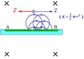
In Fig 2(b), as emitter A is charged positively and emitter B negatively, a static
electric field between them (mainly in the region above the border between A and B) is
established. The direction of the static electric field is to resist the succeeding thermal
electrons to fly from A to B.
In Fig 5, at the middle of the upper part within the tube, we show an electron with a velocityv flying rightward, and the force exerted on it by the static electric field, F,is
Fig 5,v is rightward,F is leftward; F resists the electron’s motion from A to B. A certain part of the
faster electrons emitted from A may overcome the resistance and fly across the border to fall into B.
left-ward, so the electron is decelerated by the force. Nevertheless, a certain part of the electrons emitted from A (especially the faster ones), relying on their kinetic energy, can overcome the resistance of the static electric field and travel across the border between A and B to fall into B. On arriving at B, each electron has obtained an amount of electric potential energy; of course, it is derived in exchange with the loss of an equal amount of its kinetic energy. Thus these electrons “cool down”. Consequently the two emitters and then the whole electron tube cool down (maybe very slightly), witch is compensated automatically by the heat the tube extracts from the ambient air.
In the above process, the electron tube extracts heat from a single-temperature heat reservoir (the ambient air) and all the heat is converted into electric energy without producing other effect. We maintain that the process is in contradiction to the Kelvin statement of the second law of thermodynamics.
As is well known, in 1871, to challenge the absoluteness of Clausius and Kelvin’s second law of thermodynamics, James Clerk Maxwell came up with a famous hypothesis — Maxwell’s demon (so called by Kelvin). According to Maxwell[4],
Ehrenburg [5], et al, a demon may work in either of the two following modes.
(a) In the first mode, the demon produces an (b) In the second mode, the demon produces an inequality in temperature between A and B. inequality in pressure between A and B.
Fig 6 Maxwell’s demon interferes with the random thermal motion of gas molecules*.
In the first mode, as shown in Fig 6 (a), the demon allows only the swifter molecules to pass through a small door and move from A to B, and the slower ones to pass through the small door from B to A, causing eventually a difference in temperature between A and B.
In the second mode, as shown in Fig 6 (b), the demon only allows the molecules to pass through the door from A to B, causing eventually a difference in pressure between A and B.
Maxwell’s original demon is a mechanical one.
In our present design, the magnetic field functions as a demon. It is a magnetic demon, working in the second mode: It allows thermal electrons to fly only from A to B (actually, the number of electrons migrate from A to B exceeds the one from B to A, there is a net transfer of electrons from A to B), causing a difference in electric potential between A and B, and, directly, an output current.
As is well known, applying a static magnetic field in such a way does not need expenditure of work.
2. The Actual Electron Tube Used in our Experiment
We choose Ag-O-Cs as the thermal electron emitters. Ag-O-Cs has the lowest work function among all the known thermal electron materials, about 0.8 eV, and is currently optimum in maximizing thermal electron emission at room temperature[6]. We adopted
this material and let the tube and the closed circuit (Fig 2) to operate under a uniform room temperature, so as to avoid disturbance of Seebeck effect,etc.. Ag-O-Cs cathodes are widely used in photoelectric tubes and photomultipliers, and their emission of thermal electrons (at room temperature) is usually referred to as dark current. Users certainly prefer to Ag-O-Cs cathodes of weak-dark-current. Manufacturers adjust technology and craft to produce Ag-O-Cs cathodes with weak-dark-current, usually kept in the range of 10-11 to 10-14 A/cm2. In our experiment, on the contrary, we hope to adopt Ag-O-Cs emitters of strong-dark-current. We adjusted the technology and craft repeatedly over the past 20 years and succeeded in producing Ag-O-Cs emitters with a dark current in the range of 10-7 to 10-10 A/cm2 [7].
(a) Emitters A and B, (b) Sketch of the structure (c) A photograph of FX12-51 a mica sheet, rods P, M, N, of electron tube FX12-51
two supports (yellow).
Fig 7 Electron tube FX12-51 (i.e., FX51 (12))
Between the copper bars there was a mica sheet (the green one in Fig 7 (a)), keeping A and B mutually insulated. Under the bottom of the copper bars, the mica sheet stretched out to reach the bottom glass wall, so as to prevent electrons cycling back from B to A in the space of the lower half of the tube. M, N and P were three molybdenum supporting rods. M and N were also used as electrical leads connecting A or B to a resistor outside the tube. P was 6mm above the border between A and B, and was used as a temporary anode in the tube manufacture process to oxidize the silver films on A and B by oxygen-discharge. After the manufacture of the tube, P was again used as a temporary anode to measure the dark current of the two emitters to check the quality of the tube. The typical dark current of each emitter of FX12 type tubes was 300 ~ 300,000 pA.
Finally, according to our experience, the leakage resistance between A and B should be greater than 100MΩ. The value of the leakage resistance depends chiefly on the amount of cesium input during the manufacture.
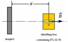
3. The Magnetic Field
The magnetic field used to deflect the orbits of the thermal electrons was produced
by a 150 mm × 100 mm × 25 mm magnet (Ceramic 8, MMPA Standard). Fig 8 shows
the magnetic induction intensity B at point O on the axis of the magnet, a distance d
apart. The B ~ d relation was measured in advance by a tesla-meter, and the results were
Fig 8 The magnetic field at point O produced by the magnet
Table 1 B ~ d relation of the magnet.
list in Table 1. In our experiment of thermo-electric conversion, the electron tube was
put at point O, within a copper shielding box, with the tube axis parallel to the magnetic
field.
d (cm) 60 50 40 35 30 25 20 15 10
B↑(N)(gauss) 0.3 1.1 2.1 2.9 4.4 7.2 13.1 25.5 59.7
B↓(S)(gauss) -0.8 -0.7 -1.6 -2.5 -4.0 -6.7 -12.7 -24.9 -58.8
4. The Experiment
Fig 9(a) is a photograph of the set up of the experiment, from left to right: a Keithley 6514 electrometer (highest current sensitivity 1×10-16A = 0.1fA), a copper shielding box (containing electron tube FX12-51), and the magnet (black). Fig 9(b) shows how the electron tube lay within the copper shielding box. The anticipated output current caused by the static magnetic field was transferred to the electrometer through a special accessory cable. Fig 9(c) is the corresponding circuit diagram.
(a) The set up: a Keithley 6514, a shielding box and a magnet (b) How the tube lay within the copper box
(c) The diagram of the current measuring circuit Fig 9 The set up of the experiment
First, chose a room temperature, which should be finely uniform and stable. Switch on the electrometer and wait a period. At that time, as the magnet was far away from the tube, d ≈ ∞, B ≈ 0, the tube should produce no output current, I ≈ 0. However,
background current changed from day to day, even from hour to hour. Fortunately, if it was changing, the change was usually slow. Sometimes, it might keep finely stable for one or two hours, even longer (such a situation was optimum for our experiment). In most cases, both the background current and its change were much smaller than the output current produced by the magnetic field. The “signal to noise ratio” is fine. Of course, the weaker the background current, the better it was for our experiment.
The influence of the earth magnetic field to this experiment was small, for convenience, we just neglected it.
We then applied a weak positive magnetic field to the tube (as shown in Fig 2(b), and denoted it by B↑, for example, d = 60cm, and B↑= 0.6 gauss. The compass placed
on the top of the copper box showed the direction of the magnetic field, which should be adjusted (very easy) to be parallel to the axis of the tube in all the steps of the whole measuring process. We observed that the tube output a weak but stable current (for example, t = 22oC, B= 0.6 gauss, I = 45fA, see table 3, page 12).
The magnetic induction intensity of the field was then increased in steps by reducing
the distance d of the tube from the magnet. For each step, we let the magnet remain
stationary for a period of at least one or two minutes, so as to exclude disturbance
of Faraday’s electromagnetic induction. We observed that, for each step, the output
current first changed quickly as the magnet arrived at a new place and kept there
stationary, then, it gradually reached a stable value. We might keep the current
unchanged as long as we wish, just by keeping the magnet stationary. And, as the
experiment going on in steps, we found, from the beginning of B↑≈0 and I ≈0, as B↑
increased step by step, the output current I (I represented the stable values of each
step) followed, until I reached a maximum value. After that, I decreased as the
magnetic field increased further. This drop down of the output current accorded with
our expectation:after the maximum current, as the magnetic field became stronger and
stronger, the radii of thermal electrons became smaller and smaller, causing the output
current to progressively reduce.
(Watch the experiment video, https://www.youtube.com/watch?v=PyrtC2nQ_UU).
through 180o around its vertical axis. The direction of the magnetic field in the copper shielding box consequently reversed. The magnetic field was now negative and might be denoted by B↓. As we expected, the direction of the output current also reversed.
We then again reduced the distance d in steps to increase the intensity of the magnetic
field B↓. The stable negative output current I for each step first increased, and then
decreased after reaching a maximum value. The situation was similar to that with the positive magnetic field.
Further experiment showed that, in each step, provided the magnetic field remained stable (i.e., provided the magnet kept stationary), the output current I would remain
stable, with a period of stability possible for as long as we wished: several minutes, several hours, even several days.
We call the output current Maxwell’s current. In general, the Maxwell’s current I for
a given FX tube depends on two factors, the temperature T and the magnetic induction
intensity B.
I = I ( B ,T ) .
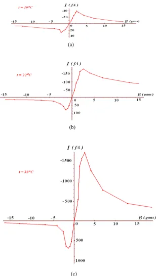
Tables 2, 3 and 4 list the data from three tests at three different temperatures, 10oC,
22oC and 33oC. Fig.10 (a), (b) and (c) were the corresponding I ~ B graphs.
d (cm) ∞ 60 50 45 40 37.5 35 30 25 20 15
B (gauss) 0 0.6 1.0 1.4 2.0 2.3 2.7 4.2 7.0 13 25
I(fA)(B↑) 4.1 9 17 25 34 39 36 26 17 8 2.7
I(fA) (B↓) 4.1 -13 -17 -20 -24 -27 -19 -15 -14 -13 -12 Table 2 I ~ B relation of FX12-51 at t = 10oC. Background current I
o = 4.1fA.
D (cm) ∞ 60 50 45 40 35 30 25 20 15
B (gauss) 0 0.6 1.0 1.4 2.0 2.7 4.2 7.0 13 25
I(fA) (B↑) 3.0 45 85 117 165 182 152 127 104 94
I(fA) (B↓) 3.0 -53 -72 -78 -59 -43 -26 -22 -20 -17
Table 3 I ~ B relation of FX12-51 at t = 22oC. Background current Io = 3.0fA.
d (cm) ∞ 60 50 45 40 35 30 25 20 15
B (gauss) 0 0.6 1.0 1.4 2.0 2.7 4.2 7.0 13 25 I(fA) (B↑) 7.7 290 560 1360 1530 1650 1270 790 440 250 I(fA) (B↓) 7.7 -520 -670 -690 -670 -270 -130 -122 -117 -115
Table 4 I ~ B relation of FX12-51at t = 32oC. Background current Io = 7.7fA.
From t = 10oC to t = 33oC (i.e., from 283K to 310K),the temperature rose only
(a)
(b)
(c)
Fig 10 The I ~ B graphs of electron tube FX12-51 at three different temperatures.
This can be finely explained by Richardson’s formula: thermal electron emission rises
very rapidly as the temperature rises,
kT W
e AT J= 2 − .
be used to measure the output voltage of the electron tube, as shown in Fig 11. The highest voltage sensitivity of Keithley 6514 is 1×10⁻⁵V = 0.01mV. The voltage here is actually the open-circuit voltage of the tube, or the electric motive force of the tube. This output voltage chiefly depends on the average kinetic energy of the thermal electrons of the emitters, in other words, depends on the temperature.
We noted in our tests that the value of the output voltage might be affected by the current leakage between the two emitters.
Fig.11 The output voltage or e.m.f. measuring circuit.
The following were the output voltages we measured with electron tube FX12-51 in a test at room temperature of T = 25oC (298K):
Background voltage B≈0, Vo = 5.6 mV.
The maximum output voltage when a magnetic field was applied to the tube was also
stable provided the magnet kept stationary. Each maximum output voltage was
measured for four times,
B↑≈ 3.5 gauss V = 20 21 20 21 mV,
B↓≈ 3.5 gauss V = -16 -18 -16 -17 mV。
According to Boltzmann’s law of equi-partition of energy, theaverage kinetic energy
of the thermal electrons at 25oC (298K) is
1.38 10 298 2
3 2
3 = × × 23×
= −
kT
ε J = 0.0385eV = 38.5emV.
In expression38.5emV, the factor 38.5mV is of the same magnitude order with the
output voltage we derived in our experiment (≈ 20mV). Therefore, we thought, the
output voltages were surely resulted from the conversion of part of the kinetic energy of
the thermal electrons.
physical quantities. In principle, a large number of such Ag-O-CS emitter pairs could be
connected in parallel to increase the output current, and connected in series to increase the output voltage, so as to build up a much greater electric power.
5. Conclusions
In the above experiment, the heat extracted by electron tube FX12-51 from the ambient air converted completely into electric energy without producing other effect. The process proved that the second law of thermodynamics was not absolutely valid, just as Maxwell and Planck had predicted more than 100 years ago[4] [8].
The authors maintain: in ordinary thermodynamic processes, just as Clausius and Kelvin pointed out correctly, entropy always increases, never decreases. Nevertheless, in some specific or extraordinary thermodynamic processes, such as our thermal electron experiment with the magnetic field, entropy does decrease.
Note: We have a continuation of this paper, with the title Realization of Maxwell’s
Hypothesis (Ⅱ), A Graphical Survey of the Various Trajectories of the Thermal
Electrons in Fu and Fu’s Experiment, see the supplement of this preprint.
REFERENCES
[1] Xinyong Fu, An Approach to Realize Maxwell’s Hypothesis,
Energy Conversion and Management, Vol.22 pp1-3 (1982).
[2] Xinyong Fu and Zitao Fu, Realization of Maxwell’s Hypothesis,
arxiv.org/physics/0311104v3 (2003 ~ 2012)
[3] Xinyong Fu and Zitao Fu, Realization of Maxwell’s Hypothesis (Ⅱ) The Right Most Problem A Graphical Survey on the Trajectories of the Thermal Electrons in Fu and
Fu’s Experiment, (2019/4)
[4] James Clerk Maxwell, Theory of Heat, P.328, (1871).
[5] W. Ehrenberg, Maxwell’s Demon,Scientific American, pp.103-110 (1967)
[6] A. H. Sommer, PHOTOEMISSIVE MATERIALS, Preparation, Properties, and Use,
John Wiley & Sons (1968), Section 10.7.1, Chapter 10.
Cs, Journal of Applied Physics, Volume 28, Number 9, p.1031 (1957)
[8] Max Planck, Forlesungen Uber Thermodynamik (Erste auflage,1897; Siebente
auflage,(1922),§116 &§136.
English Version: TreatiseOn Thermodynamics, Dover Publications Inc. (1926),§116