Suitable Combination of Direct Intensity Modulation and Spreading Sequence for LIDAR with pulse coding

(1)

Suitable Combination of Direct Intensity Modulation

and Spreading Sequence for LIDAR with Pulse

Coding

Gunzung Kim and Yongwan Park *

Department of Information and Communication Engineering, Yeungnam University, 280 Daehak-Ro, Gyeongsan, Gyeongbuk 38541, Republic of Korea; gzkim@yu.ac.kr

* Correspondence: ywpark@yu.ac.kr; Tel.: +82-53-810-3942

Abstract: In the coded pulse scanning light detection and ranging (LIDAR) system, the number of laser pulses used at a given measurement point changes depending on the modulation and the method of spreading used in optical code-division multiple access (OCDMA). The number of laser pulses determines the pulse width, output power, and duration of the pulse transmission of a measurement point. These parameters determine the maximum measurement distance of the laser and the number of measurement points that can be employed per second. In this paper, we suggest possible combinations of modulation and spreading technology that can be used for OCDMA, evaluate the performance and characteristics of them, and study optimal combinations according to varying operating environments.

Keywords:LIDAR; time-of-flight; IM/DD OCDMA; free-space optical communication; modulation; spreading code

Key Contribution:We suggest possible combinations of modulation and spreading technology that can be used for OCDMA, evaluate the performance and characteristics of them, and study optimal combinations according to varying operating environments.

1. Introduction

Pulse scanning light detection and ranging (LIDAR) measures the distance to a given object using a time-of-flight (ToF) technique that calculates the time required for a pulse to transmit to and reflect off the object [1–6]. The distance image of the surroundings can be generated with excellent angular resolution and is used to determine the area that can be traveled while mounted on an autonomous vehicle or an autonomous mobile robot. Many factors determine the operating characteristics of pulse scanning LIDAR and can be divided into characteristics of the transmission and generation of a pulse, and those of the reception of a reflected pulse [3,7,8]. In the transmitter, the pulse scanning LIDAR determines the wavelength of the laser as well as pulse width, interval, and peak power [9]. In the receiver, it determines the size of the receiving aperture, and uses a photodetector, a pulse detection method, the threshold-to-noise ratio (TNR), and a range estimation method [10–13]. The characteristics used to generate pulses in the transmitter are limited by the maximum permissible exposure (MPE) to comply with eye safety standards [14]. The most critical parameter that determines the maximum measurement distance in LIDAR is the pulse peak power of the transmitter and the TNR of the receiver. As the strength of the received signal is proportional to the peak power of the pulse and inversely proportional to the square of the measured distance, the higher the pulse peak power and the lower the TNR, the greater the distance that can be measured. Thus, if the characteristics of one parameter are improved, the characteristics of the other parameters worsen [9]. Depending on the primary purpose of LIDAR, one or two of parameters are used as characteristics of preference, and the remaining are rendered MPE compliant.

(2)

Some studies have focused on solving the range ambiguity of pulse scanning LIDAR by used pulse coding to avoid crosstalk [15–19] or mutual interference that occurs when two or more LIDARs simultaneously operate [18–20]. Such LIDARs measure distances using multiple pulses generated by random sequences [15–17] or specially designed codes [18–20], rather than one pulse per measurement point. Even if multiple pulses are used, the parameters that determine the characteristics of the transmitter in the conventional pulse scanning scheme are maintained. To comply with eye safety standards, the pulse peak power is distributed across several pulses so that the energy allocated to a pulse decreases in inverse proportion to the number of pulses, and the time required to transmit pulses at a given measurement point is proportional to the number of pulses [18–20]. The use of multiple pulses also enhances the accuracy of the distance measurement [19].

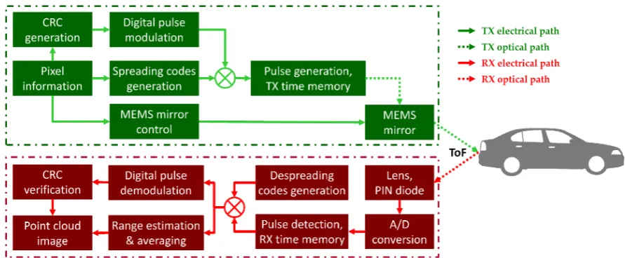
In LIDAR with pulse coding [18,19], the number of pulses used at a measurement point is determined by the modulation method and the spreading code method, as illustrated in Figure1. The optical channel differs significantly from radio frequency (RF) channels. Unlike RF systems, where the amplitude, frequency, and phase of the carrier signal are modulated, the intensity of the optical carrier is modulated in optical systems. In an optical wireless communication system using unipolar signaling, the numbers and positions of the pulses to be transmitted and empty slots are determined by the modulation and spreading code methods used [21–25]. To accurately demodulate and despread the signal at the receiver of the code pulse LIDAR, both the numbers and the positions of the pulses and the empty slots are used. In a unipolar optical communication system, on–off keying (OOK), pulse position modulation (PPM), differential PPM (DPPM), multipulse PPM (MPPM), digital pulse interval modulation (DPIM), and dual-header pulse interval modulation (DH-PIM) are widely used as modulation techniques, and prime code (PC) and optical orthogonal code (OOC) are widely used as spreading code techniques [21–23]. The number of pulses, pulse peak power, average signal-to-noise ratio (SNR), maximum measurable distance, accuracy and precision of the measured distance, and packet error rate (PER) vary depending on the combination of modulation scheme and spreading code scheme used. In this paper, we investigate the characteristics of various modulations and spreading code methods that can be used for LIDAR with pulse coding and compare various characteristics of LIDAR according to the combinations.

(3)

2. Digital modulation and spreading codes

2.1. Digital pulse modulation schemes

Because the average optical power of LIDAR is constrained, it is useful to determine a modulation scheme that can provide the requisite bandwidth and use power efficiently. Many digital modulation schemes have been proposed for use in optical wireless communication systems. Given the requirements, the performance of a communication system depends on how the information is represented in the modulation scheme. Types of modulation are thus the critical determinant of system design. In digital modulation schemes, information is embedded in both mark and space periods, and encoding is a term in discrete time slots. Each discrete amplitude of a modulated signal appears by varying the characteristics of the pulse at a discrete time. Such time characteristics as pulse position, width, and spacing are modulated using the instantaneous modulation signal but a constant sampling frequency is sustained. The OOK provides higher bandwidth efficiency but poor optical power performance. Digital pulse time modulation techniques such as PPM, DPPM, MPPM, DPIM, and DH-PIM are recognized as block codes through the OOK, which provides a balance between bandwidth and optical power efficiency [23]. Digital modulation schemes can be divided into two main categories: isochronous and anisochronous. In an isochronous mode, the length of the symbol is fixed; in the anisochronous mode, the length of the symbol is variable. The OOK, PPM, and MPPM are isochronous, whereas the DPPM, DPIM, and DH-PIM are anisochronous. An illustration of the overall conversion method and the time waveforms of modulation techniques with fixed pulse width that are discussed–the OOK, PPM, DPPM, MPPM, DPIM, and DH-PIM–are shown in Figure2.

Figure 2.Time waveforms for OOJ, PPM, DPPM, MPPM, DPIM, and DH-PIM signals.ETXis the pulse peak power,Tfis the block duration, andTsis the time slot duration.

(4)

NRZ-OOK, the pulses fill the entire bit duration; and in RZ-OOK, they occupy a particular portion of the bit duration. Owing to the relatively wide pulse, NRZ-OOK has higher bandwidth efficiency but lower power efficiency than RZ-OOK. In the OOK, symbols are displayed as amplitude pulse groups. A combination of an M-bit input block with symbols for on or off can representL = 2M unique combinations. Three significant advantages of the OOK are that it provides a high SNR, low distortion performance, and superior system linearity, all of which are independent of channel quality. In the PPM, each bit of anM-bit input block is mapped to one ofL=2Mpossible symbols [23,26– 30]. A frame consists of a pulse that occupies a slot, and the remaining slots have no pulse. Therefore, the information is displayed as pulse position within the same symbol as the decimal value of the M-bit input block. Because the PPM requires both slot and symbol synchronization at the receiver to demodulate the signal, it delivers impressive optical power performance but at the cost of bandwidth and circuit simplicity.

The MPPM is a generalization of the PPM that allows more than one pulse per symbol. Moreover, w-pulsen-slot MPPM has(nw)unique symbols that correspond to fillingnslots withwpulses in a frame [26,28–36]. As the level of coding increases, the number of PPM slots and the required transmission bandwidth both increase exponentially. To overcome these limitations, the MPPM was introduced as a way to improve the bandwidth utilization of the PPM. This approach reduces the bandwidth to half of that in the traditional PPM at the same transmission efficiency. That is, a single frame can carry information of size log₂(nw)bits. On the contrary, for the PPM, this rate is log₂L bits. The amount of information that the MPPM can transfer increases with the number of pulses in the fixed-length frame. The disadvantage is that if one or more of these pulses are erroneous, the frame is incorrectly demodulated. Therefore, too many source bits are affected. The MPPM provides information capacity twice as poor as that of the PPM and is inferior to it in terms of error performance.

In the DPPM,M=log₂L-bit input block maps to one ofLunique DPPM symbols, including a pulse andL−1 empty slots [26–28,30,37,38]. The DPPM symbol is derived from the corresponding PPM symbol by removing all empty slots following the pulse, thus reducing the average symbol length and increasing bandwidth efficiency. The DPPM indicates its own symbol synchronization when all symbols end with a pulse. For a long sequence of zeros, there may be a slot synchronization problem that can be handled using a guard slot (GS) immediately after the pulse is removed. The DPPM improves bandwidth and power efficiency over the PPM for fixed average bit rate and fixed available bandwidth.

The DPIM has built-in symbol synchronization that improves bandwidth efficiency and data speed compared with the PPM, and power efficiency compared with the OOK [23,26–28,30]. The waveform of the DPIM is similar to that of the DPPM except that the variable frame length and the pulse are located at the beginning of the frame. In the DPIM, each symbol starts with a pulse of short duration after the optional GS followed by the number of empty time slots, which is determined by the decimal value of the bit input block. In other words, a symbol is represented by a discrete interval between consecutive pulses belonging to two consecutive frames. The GS consists of zero or more empty slots and is vital to avoiding continuous pulses when the input symbol is zero. The frame length of the DPIM may vary depending on the bit input block. In the DPIM, anM-bit input block of duration Tf (whereTf =MTb,Tbis an equivalent binary bit period) is represented by a single pulse located in one of theL=2Mtime slots. The speeds of the DPIM and DPPM slots increase exponentially with OOK bit rates as bit resolution increases. If two systems are included in the GS, this increase is even greater. As the slot frequency increases, bandwidth requirements also increase.

In DH-PIM, a symbol consists of two sections: a heading that starts a symbol and an ending information section. Thenth symbolSn(hn,dn)starts with the headerhnof the durationTh= (α+1)Ts and ends with the sequence ofdnempty slots, whereα>0 is an integer [23,26,27]. Depending on the most significant bit (MSB) of the input block, two headers are considered,H1andH2, corresponding

(5)

the decimal value of the input block if the symbol starts withH1. If the symbol starts withH2, it is

the decimal value of the 1’s complement of the input code word. The header pulses play the dual role of symbol initiation and time reference for the preceding and succeeding symbols, resulting in built-in symbol synchronization. In other words, DH-PIM creates a symbol to enable built-in symbol synchronization. Thus, like the PPM symbol, the DH-PIM removes the extra time slot after the pulse and increases the average symbol length compared with the PIM, thus increasing data throughput.

Comparisons of modulation techniques wth fixed pulse width are based on various parameters, such as bandwidth occupancy, distortion, SNR, suitability for transmission channels, and error probability. No scheme yields optimal performance and negotiates all signals. For optical transmission, digital pulse time modulation techniques are preferred because of their high peak power and low average power characteristics. They require higher bandwidth than the OOK and provide a higher SNR. The disadvantage of digital pulse time modulation techniques is that they require symbol synchronization and, therefore, more circuitry than other approaches. Tables1and2summarize the characteristics ofM-bit input blocks when they are converted into symbols by the OOK, PPM, DPPM, MPPM, DPIM, and DH-PIM, whereRbis the bit rate andN0is the energy of noise [23,26–31,34,35,37,38].

In case of optical communication, the influence of path loss can be ignored, and the received average energy is converted into the maximum energy transmitted, and the received energy per bitEb, received energy per symbolEs, and power efficiencyηpare calculated by using this. On the contrary, in case of LIDAR, the maximum energy to be emitted is fixed, and the reflected signal from the object is received. Thus, the influence of path loss must be reflected in the received energy. Therefore, in this paper, energyETXemitted from LIDAR is reflected off the surface of an object at a distance ofRaway, and the received energyERXis calculated by Equation1. The symbol error rate (SER) is calculated by Equation2, and the PER by Equation3using ERX, which is the received energy according to each modulation technique. Table3summarizes the error probability of the digital pulse modulation techniques [23,26,29–31,34,35,37,39–41]. The symbol error ratePseis optimum when the threshold factorkis 0.5.

ERX =ETX

πτ0τ_a2D2_RρT 4R2_θ

R

(1)

Pse=P0Pe0+P1Pe1=P0Q k

s

Es 2N0

!

+ (1−P0)Q (1−k)

s

Es 2N0

!

(2)

Ppe =1−(1−Pse)

Npkt¯L

M _≈ Npkt

¯ L

M Pse (3)

Table 1.Comparison of basic characteristics of digital pulse modulation techniques

Modulation Number of bits (M)

Maximum number of bits (Np)

Number of possible

unique symbols (L)

Maximum number of time slots

(Lmax)

Average symbol length ( ¯L)

Slot duration

(Ts)

NRZ-OOK M M 2M M M _R1

b

PPM M 1 2M LPPM LPPM R1b

DPPM M 1 2M LDPPM LDPPM₂ +1 _R1_b

MPPM blog₂Lc w (_wn) n n _R1

b DPIM M 1 2M LDPI M LDPI M₂ +1 R1b

DH-PIM M 2 2M 2M−1+α 2

M−1₊₂ α+1

(6)

Table 2.Comparison of power characteristics of digital pulse modulation techniques

Modulation

Bandwidth requirements

(Breq)

Peak-to-average power ratio

(PAPR)

Peak current

(Ip)

Energy of a pulse

(Ep)

Energy of a bit

(Eb)

NRZ-OOK Rb 2 2 ¯ERX_OOK

4 ¯E2 RX_OOK

Rb

4 ¯E2 RX_OOK

Rb

PPM MRb

LPPM LPPM LPPME¯RX_PPM L2

PPME¯2RX_PPM Rb

L3

PPME¯2RX_PPM MRb

DPPM 2MRb

LDPPM+1 2 2 ¯ERX_DPPM

4 ¯E2 RX_DPPM

Rb

4 ¯E3 RX_DPPM

Rb

MPPM MRb

n 2 2 ¯ERX_MPPM 4 ¯E 2 RX_MPPM

Rb

4 ¯E3 RX_MPPM

Rb

DPIM 2MRb

LDPI M+1 2 2 ¯ERX_DPI M

4 ¯E2 RX_DPI M

Rb

4 ¯E3 RX_DPI M

Rb

DH-PIM 2MRb

2M−1₊₂_α₊₁ 2 2 ¯ERX_DH−PI M

4 ¯E2 RX_DH−PI M

Rb

4 ¯E3 RX_DH−PI M

Rb

Table 3.Comparison of error probabilities of digital pulse modulation techniques

Modulation

Probability of "0"

(P0)

Probability of "1"

(P1)

Marginal probability

(Pe0)

Optimum symbol error probability

(Pse−opt)

NRZ-OOK 1₂ 1₂ QkE_√¯RX_OOK

N0Rb

QE¯RX_OOK

2√N0Rb

PPM LPPM−1 LPPM

1

LPPM Q

_kL

PPM_√E¯RX_PPM N0Rb

QLPPME¯RX_PPM

2√N0Rb

DPPM LDPPM−1 LDPPM+1

2

LDPPM+1 Q

_k₍_L

LPPM+1)E¯RX_DPPM

2√N0Rb

Q(LDPPM+1)E¯RX_DPPM

4√N0Rb

MPPM n−_nw w_n QknE¯RX_MPPM

w√N0Rb

QnE¯RX_MPPM

4w√N0Rb

DPIM LDPI M−1

LDPI M+1

2

LDPI M+1 Q

_k

(LDPI M+1)E¯RX_DPI M

2√N0Rb

Q(LDPI M+1)E¯RX_DPI M

4√N0Rb

DH-PIM 4 ¯LDH−PI M−3α

¯

LDH−PI M

3α

¯

LDH−PI M Q

2k(2M−1₊₂

α+1)_E¯_RX_{_}_DH₋_{PI M} 3α √ N0Rb Q

(2M−1₊₂

α+1)_E¯_RX_{_}_DH₋_{PI M} 3α

√

N0Rb

2.2. One-dimensional optical spreading codes

(7)

all be assumed to be OOC code sets, as long as the code set correlation constraints are met. The code generation of OOC(N, 3, 1)and OOC(31, 3, 1)are shown Tables4and5, respectively.

Table 4.OOC(N, 3, 1)sequence indices for various lengths

N Sequence index, whenN≤49

7 {1, 2, 4}

13 {1, 2, 5},{1, 3, 8}

19 {1, 2, 6},{1, 3, 9},{1, 4, 11} 25 {1, 2, 7},{1, 3, 10},{1, 4, 12},{1, 5, 14} 31 {1, 2, 8},{1, 3, 12},{1, 4, 16},{1, 5, 15},{1, 6, 14} 37 {1, 2, 12},{1, 3, 10},{1, 4, 18},{1, 5, 13},{1, 6, 19},{1, 7, 13} 43 {1, 2, 20},{1, 3, 23},{1, 4, 16},{15, 14},{1, 6, 17},{1, 7, 15},{1, 8, 19}

Table 5.OOC(31, 3, 1)sequences

Index Sequence code

{1, 2, 8} 11000 00100 00000 00000 00000 00000 0 {1, 3, 12} 10100 00000 01000 00000 00000 00000 0 {1, 4, 16} 10010 00000 00000 10000 00000 00000 0 {1, 5, 15} 10001 00000 00001 00000 00000 00000 0 {1, 6, 14} 10000 10000 00010 00000 00000 00000 0

Compared with OOC, the PC generation process is relatively simple. A code set with a code length ofn=p2_{and code weight}_w₌_p_has_p_{unique sequences [21,24,25]. An example of a PC set}

withp=5 is shown in Table6. The main disadvantage of PC is that the number of available codes is limited. The code length of PC is onlyp2, which may affect the system’s performance in terms of bit error rate (BER) and multiple access interference (MAI). Therefore, longer codes that maintain desirable properties are beneficial.

Table 6.Prime code (PC) sequences whenp=5

Groups i

PC sequence PC sequence code

x 0 1 2 3 4

0 0 0 0 0 0 S0 C0=10000 10000 10000 10000 10000

1 0 1 2 3 4 S1 C1=10000 01000 00100 00010 00001

2 0 2 4 1 3 S2 C2=10000 00100 00001 01000 00010

3 0 3 1 4 2 S3 C3=10000 00010 01000 00001 00100

4 0 4 3 2 1 S4 C4=10000 00001 00010 10000 01000

As the cardinality of the PC corresponds to the number of users,M, it is equal tow, of the PC, andwis equal to the prime numberp; thus,pmust be increased. To increase the number of users on the network, weightwmust be greater. A modified prime code (MPC) has been proposed to overcome the drawbacks of the PC [21,24,25,45]. This optical sequence eliminates some redundant pulses from the original PC with a pulse, assuming a BER requirement such as 10−9and a certain number of users. The weight of the MPC is smaller than that of the PC, but the code can support thepgroup containing

(8)

Table 7.Modified prime code (MPC) sequencesS0_iconstructed forp=5 andw=4

Groups i

MPC sequence MPC sequence code

x a0 a1 a2 a3

0 0 0 0 0 S0₀ C0₀=10000 10000 10000 10000 00000 1 0 1 2 3 S0₁ C0₁=10000 01000 00100 00010 00000 2 0 2 4 1 S0₂ C0₂=10000 00100 00001 01000 00000 3 0 3 1 4 S0₃ C0₃=10000 00010 01000 00001 00000 4 0 4 3 2 S0₄ C0₄=10000 00001 00010 10000 00000

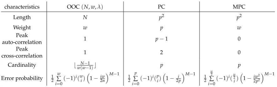
Table8summarizes the characteristics of OOC, PC, and MPC including length, weight, peak auto-correlation and cross-correlation, cardinality, and error probability [21,24,25,42–52].

Table 8.Performance comparison of optical spreading codes

characteristics OOC(N,w,λ) PC MPC

Length N p2 p2

Weight w p w

Peak

auto-correlation 1 p−1 0

Peak

cross-correlation 1 2 0

Cardinality b N−1

w(w−1)c p p

Error probability 1₂ ∑w

i=0

(−1)i(w_i)1−iw

2n M−1

1 2

p

∑

i=0

(−1)i(p_i)1− i

2p M−1

1 2

w 2

∑

i=0

(−1)i(w2 i)

1−iw2

2p2 M−1

3. Performance evaluation of combinations of modulation and spreading code techniques

3.1. Combinations of modulation and spreading code techniques

To evaluate the performance of the modulation and spreading code schemes used in the prototype LIDAR system, several operating conditions have been specified according to the characteristics of the prototype LIDAR system [18,19]. At each pixel, the prototype LIDAR system generates pixel information to identify the measuring point and emission time. Pixel information is represented by a nine-bit stream consisting of a leading "1," a five-bit column identification number (CID), and a three-bit cyclic redundancy check (CRC) checksum. The CID represents the locations of corresponding pixels for each measurement angle and identifies each of the 30 columns from a 30×30 range image.

• A nine-bit block is used to identify each measurement point, and the first bit is always "1" • Up to five measurement points can be measured simultaneously

• Pulse width is fixed at 5 ns and pulse transmission is completed within 67 µs • The maximum output of the laser pulse is eye-safety class 1 compliant • The maximum desired distance: 150 m

• Range gate: 1 µs

• Probability of false alarm: 0.5 • False alarm rate: 500.000/s • TNR: 9.8 dB

(9)

can be known by the number of "0s" transmitted before "1" is reached. The DPIM and DH-PIM can identify symbols with a number of "0s" after a "1" and cannot know the symbols because the number of "0s" in the last symbol is unknown. In this case, we should mark the end of the transmission by appending a trailing "1" to the end of the last symbol. We use zero GSs for the modulation techniques because optical spreading codes are very sparse codes, and two or more successive "0s" precede a very sparse "1."

Table 9.Three-bit block representation according to modulation technique

Source symbol OOK 8-PPM 8-DPPM 2-5MPPM 8-DPIM 8-DH-PIM2

0 000 10000000 1 10001 1 100

1 001 01000000 01 01100 10 1000

2 010 00100000 001 01001 100 10000

3 011 00010000 0001 10010 1000 100000

4 100 00001000 00001 11000 10000 110000

5 101 00000100 000001 00101 100000 11000

6 110 00000010 0000001 00011 1000000 1100

7 111 00000001 00000001 10100 10000000 110

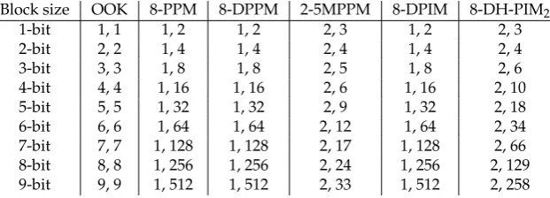
The possible modulation schemes according to the size of the bit input block are shown in Table10. As slot size increases, the number of slots required for modulation increase linearly in the OOK, but those in the PPM, DPPM, DPIM, and DH-PIM increase exponentially, and that of the MPPM increases exponentially but relatively mildly.

Table 10.Possible modulation schemes according to the size of the bit input block

Block size OOK 8-PPM 8-DPPM 2-5MPPM 8-DPIM 8-DH-PIM2

1-bit 1, 1 1, 2 1, 2 2, 3 1, 2 2, 3

2-bit 2, 2 1, 4 1, 4 2, 4 1, 4 2, 4

3-bit 3, 3 1, 8 1, 8 2, 5 1, 8 2, 6

4-bit 4, 4 1, 16 1, 16 2, 6 1, 16 2, 10

5-bit 5, 5 1, 32 1, 32 2, 9 1, 32 2, 18

6-bit 6, 6 1, 64 1, 64 2, 12 1, 64 2, 34

7-bit 7, 7 1, 128 1, 128 2, 17 1, 128 2, 66

8-bit 8, 8 1, 256 1, 256 2, 24 1, 256 2, 129

9-bit 9, 9 1, 512 1, 512 2, 33 1, 512 2, 258

(10)

Table 11.Possible block partitioning according to modulation techniques. A bold "1" shows a leading "1" or a trailing "1."

Block paritioning OOK PPM DPPM MPPM DPIM DH-PIM2

1: 2 : 2 : 2 : 2 9, 9 5, 17 5, 17 9, 17

2 : 2 : 2 : 2 :1 5, 17 9, 17

1: 2 : 3 : 3 9, 9 4, 21 4, 21 7, 15

2 : 3 : 3 :1 4, 21 7, 17

1: 4 : 4 9, 9 3, 33 3, 33 5, 13

4 : 4 :1 3, 33 5, 21

1: 5 : 3 9, 9 3, 41 3, 41 5, 15

5 : 3 :1 3, 41 5, 25

1: 8 9, 9 2, 257 2, 257 3, 25

8 :1 2, 257 3, 131

The combination of modulation and spreading code techniques is determined to satisfy all operating conditions of the prototype LIDAR. The following operating characteristics are determined according to the combinations:

• Symbol stream

• Block size and partitioning • Pulse peak power

• Number of time slots • Number of pulses • leading "1" or trailing "1"

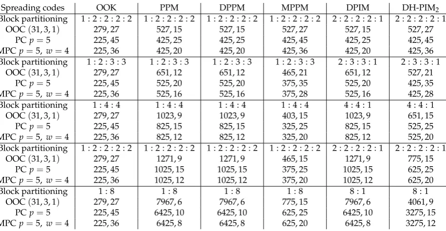
If the bit input block is divided into partitions of various sizes and the optical spreading code with a cardinality of five is applied, the transmission characteristics are as shown in Tables12and13. The number of time slots needed for transmission is the greatest, and each pair relates the number of slots, the number of pulses, and the maximum pulse output. The transmission power of the pulse is inversely proportion to the number of transmitted pulses.

Table 12.Number of pulses and time slots as combination of modulation and spreading code

Spreading codes OOK PPM DPPM MPPM DPIM DH-PIM2

Block partitioning 1 : 2 : 2 : 2 : 2 1 : 2 : 2 : 2 : 2 1 : 2 : 2 : 2 : 2 1 : 2 : 2 : 2 : 2 2 : 2 : 2 : 2 : 1 2 : 2 : 2 : 2 : 1

OOC(31, 3, 1) 279, 27 527, 15 527, 15 527, 27 527, 15 527, 27

PCp=5 225, 45 425, 25 425, 25 425, 45 425, 25 425, 45

MPCp=5, w=4 225, 36 425, 20 425, 20 425, 36 425, 20 425, 36

Block partitioning 1 : 2 : 3 : 3 1 : 2 : 3 : 3 1 : 2 : 3 : 3 1 : 2 : 3 : 3 2 : 3 : 3 : 1 2 : 3 : 3 : 1

OOC(31, 3, 1) 279, 27 651, 12 651, 12 465, 21 651, 12 527, 21

PCp=5 225, 45 525, 20 525, 20 375, 35 525, 20 425, 35

MPCp=5, w=4 225, 36 525, 16 525, 16 375, 28 525, 16 425, 28

Block partitioning 1 : 4 : 4 1 : 4 : 4 1 : 4 : 4 1 : 4 : 4 4 : 4 : 1 4 : 4 : 1

OOC(31, 3, 1) 279, 27 1023, 9 1023, 9 403, 15 1023, 9 651, 15

PCp=5 225, 45 825, 15 825, 15 325, 25 825, 15 525, 25

MPCp=5, w=4 225, 36 825, 12 825, 12 325, 20 825, 12 525, 20

OOC(31, 3, 1) 279, 27 1271, 9 1271, 9 465, 15 1271, 9 775, 15

PCp=5 225, 45 1025, 15 1025, 15 375, 25 1025, 15 625, 25

MPCp=5, w=4 225, 36 1025, 12 1025, 12 375, 20 1025, 12 625, 20

Block partitioning 1 : 8 1 : 8 1 : 8 1 : 8 8 : 1 8 : 1

OOC(31, 3, 1) 279, 27 7967, 6 7967, 6 775, 15 7967, 6 4061, 9

PCp=5 225, 45 6425, 10 6425, 10 625, 25 6425, 10 3275, 15

(11)

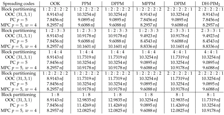
Table 13.Number of pulses and time slots as combination of modulation and spreading code

Block partitioning 1 : 2 : 2 : 2 : 2 1 : 2 : 2 : 2 : 2 1 : 2 : 2 : 2 : 2 1 : 2 : 2 : 2 : 2 2 : 2 : 2 : 2 : 1 2 : 2 : 2 : 2 : 1 OOC(31, 3, 1) 8.9143 nJ 10.3254 nJ 10.3254 nJ 8.9143 nJ 10.3254 nJ 8.9143 nJ

PCp=5 7.8456 nJ 9.0895 nJ 9.0895 nJ 7.8456 nJ 9.0895 nJ 7.8456 nJ MPCp=5, w=4 8.2957 nJ 9.6088 nJ 9.6088 nJ 8.2957 nJ 9.6088 nJ 8.2957 nJ Block partitioning 1 : 2 : 3 : 3 1 : 2 : 3 : 3 1 : 2 : 3 : 3 1 : 2 : 3 : 3 2 : 3 : 3 : 1 2 : 3 : 3 : 1

OOC(31, 3, 1) 8.9143 nJ 10.9178 nJ 10.9178 nJ 9.4923 nJ 10.9178 nJ 9.4923 nJ PCp=5 7.8456 nJ 9.6088 nJ 9.6088 nJ 8.4543 nJ 9.6088 nJ 8.4543 nJ MPCp=5, w=4 8.2957 nJ 10.1601 nJ 10.1601 nJ 8.8336 nJ 10.1601 nJ 8.8336 nJ Block partitioning 1 : 4 : 4 1 : 4 : 4 1 : 4 : 4 1 : 4 : 4 4 : 4 : 1 4 : 4 : 1

OOC(31, 3, 1) 8.9143 nJ 11.7319 nJ 11.7319 nJ 10.3254 nJ 11.7319 nJ 10.3254 nJ PCp=5 7.8456 nJ 10.3254 nJ 10.3254 nJ 9.0895 nJ 10.3254 nJ 9.0895 nJ MPCp=5, w=4 8.2957 nJ 10.9178 nJ 10.9178 nJ 9.6088 nJ 10.9178 nJ 9.6088 nJ

Block partitioning 1 : 2 : 2 : 2 : 2 1 : 2 : 2 : 2 : 2 1 : 2 : 2 : 2 : 2 1 : 2 : 2 : 2 : 2 2 : 2 : 2 : 2 : 1 2 : 2 : 2 : 2 : 1 OOC(31, 3, 1) 8.9143 nJ 11.7319 nJ 11.7319 nJ 10.3254 nJ 11.7319 nJ 10.3254 nJ

PCp=5 7.8456 nJ 10.3254 nJ 10.3254 nJ 9.0895 nJ 10.3254 nJ 9.0895 nJ MPCp=5, w=4 8.2957 nJ 10.9178 nJ 10.9178 nJ 9.6088 nJ 10.9178 nJ 9.6088 nJ

OOC(31, 3, 1) 8.9143 nJ 12.9835 nJ 12.9835 nJ 10.3254 nJ 12.9835 nJ 11.7319 nJ PCp=5 7.8456 nJ 11.4269 nJ 11.4269 nJ 9.0895 nJ 11.4269 nJ 10.3254 nJ MPCp=5, w=4 8.2957 nJ 12.0825 nJ 12.0825 nJ 9.6088 nJ 12.0825 nJ 10.9178 nJ

3.2. Performance evaulation of combined techniques

The experimental environment was the same as that for the prototype LIDAR system, and a modulation technique and a spreading code technique was used. Experiments were conducted using various parameters on a table with a 2×2m white paper wall as shown in Figure3. We evaluated the performance of the following elements based on combinations of various modulation and spreading code techniques as well as the operating characteristics of the prototype LIDAR system [18,19].

Figure 3.Experimental conditions and optical structure of the prototype LIDAR systems

(12)

standards for digital elevation data [54,55]. The maximum measurement distance of the pulse was proportional to the number of transmitted pulses, as were accuracy and precision .

Table 14.Maximum distance as a combination of modulation and spreading code

OOC(31, 3, 1) 95 m 102 m 102 m 95 m 102 m 95 m

PCp=5 89 m 96 m 96 m 89 m 96 m 89 m

MPCp=5, w=4 91 m 98 m 98 m 91 m 98 m 91 m

OOC(31, 3, 1) 95 m 105 m 105 m 98 m 105 m 98 m

PCp=5 89 m 98 m 98 m 92 m 98 m 92 m

MPCp=5, w=4 91 m 101 m 101 m 94 m 101 m 94 m

OOC(31, 3, 1) 95 m 109 m 109 m 102 m 109 m 102 m

PCp=5 89 m 102 m 102 m 96 m 102 m 96 m

MPCp=5, w=4 91 m 105 m 105 m 98 m 105 m 98 m

OOC(31, 3, 1) 95 m 109 m 109 m 102 m 109 m 102 m

PCp=5 89 m 102 m 102 m 96 m 102 m 96 m

MPCp=5, w=4 91 m 105 m 105 m 98 m 105 m 98 m

OOC(31, 3, 1) 95 m 114 m 114 m 102 m 114 m 109 m

PCp=5 89 m 107 m 107 m 96 m 107 m 102 m

MPCp=5, w=4 91 m 110 m 110 m 98 m 110 m 105 m

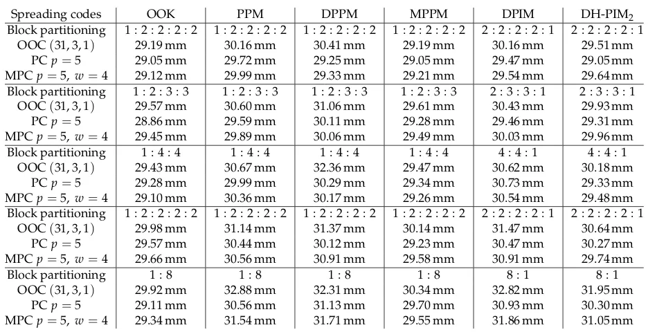
Table 15.Accuracy as a combination of modulation and spreading code

Block partitioning 1 : 2 : 2 : 2 : 2 1 : 2 : 2 : 2 : 2 1 : 2 : 2 : 2 : 2 1 : 2 : 2 : 2 : 2 2 : 2 : 2 : 2 : 1 2 : 2 : 2 : 2 : 1 OOC(31, 3, 1) 29.19 mm 30.16 mm 30.41 mm 29.19 mm 30.16 mm 29.51 mm

PCp=5 29.05 mm 29.72 mm 29.25 mm 29.05 mm 29.47 mm 29.05 mm

MPCp=5, w=4 29.12 mm 29.99 mm 29.33 mm 29.21 mm 29.54 mm 29.64 mm Block partitioning 1 : 2 : 3 : 3 1 : 2 : 3 : 3 1 : 2 : 3 : 3 1 : 2 : 3 : 3 2 : 3 : 3 : 1 2 : 3 : 3 : 1 OOC(31, 3, 1) 29.57 mm 30.60 mm 31.06 mm 29.61 mm 30.43 mm 29.93 mm

MPCp=5, w=4 29.45 mm 29.89 mm 30.06 mm 29.49 mm 30.03 mm 29.96 mm Block partitioning 1 : 4 : 4 1 : 4 : 4 1 : 4 : 4 1 : 4 : 4 4 : 4 : 1 4 : 4 : 1

OOC(31, 3, 1) 29.43 mm 30.67 mm 32.36 mm 29.47 mm 30.62 mm 30.18 mm

MPCp=5, w=4 29.10 mm 30.36 mm 30.17 mm 29.26 mm 30.54 mm 29.48 mm Block partitioning 1 : 2 : 2 : 2 : 2 1 : 2 : 2 : 2 : 2 1 : 2 : 2 : 2 : 2 1 : 2 : 2 : 2 : 2 2 : 2 : 2 : 2 : 1 2 : 2 : 2 : 2 : 1

MPCp=5, w=4 29.66 mm 30.56 mm 30.91 mm 29.58 mm 30.91 mm 29.74 mm

(13)

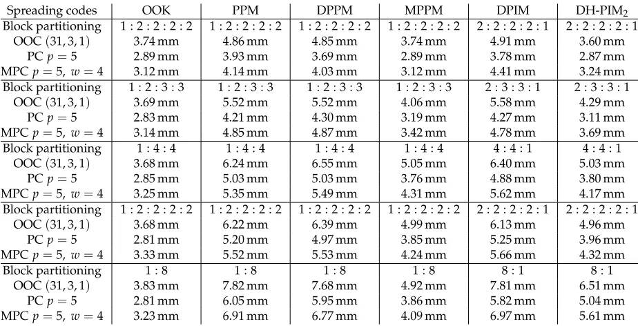
Table 16.Precision as a combination of modulation and spreading code

OOK allocates one time slot per bit, so the number of time slots is constant regardless of the partitioning of the block. PPM, DPPM, and DPIM are different from each other in their numbers of "1s" and their average symbol sizes, but their number of time slots is the same according to the maximum symbol size, indicating whether a transmission is possible within a given time. These three modulation methods are identical regarding the parameters required to measure the performance of the LIDAR system, even though the symbol representation is different. The DH-PIM has the advantage that the average and maximum symbol sizes are both smaller than those of PPM, DPPM, and DPIM. However, it has a disadvantage that the number of "1s" required for representing a block is large. If the number of slots corresponding to "1" is large, the pulse peak power is small, and the maximum measurement distance is shortened, but the accuracy and precision are improved. Unlike other modulation methods in which the number of "1s" is fixed, DH-PIM changes the number of "1s" according to the symbol. If the pulse peak power can be changed dynamically according to the number of "1s", a longer pulse distance can be measured using the pulse peak power when the number of "1s" is small. MPPM has the advantage that the average and maximum symbol sizes are the smallest modulation schemes. However, as in the case of DH-PIM, the number of "1s" needed to represent a symbol is increased, so the pulse peak power is reduced. As a result, the maximum measurement distance is shortened, but accuracy and precision are improved. Compared to other modulation methods, MPPM exhibits the best balance of measurement distance, precision, and accuracy.

(14)

in the LIDAR system, it is best to use the combination with the least number of pulses satisfying the maximum allowable transmission time. Of the combinations we evaluated, the combination of using PPM, DPPM, or DPIM as the modulation technique and using OOC as the spreading code technique can measure the farthest distance. Figure4shows the overall relationship between the measured results and combinations of modulation and spreading codes.

85

90

95

100

105

110

115 Distance (m)

28.5

29

29.5

30

30.5

31

31.5

32

32.5

33 Accuracy (mm)

OOK-OOC OOK-PC OOK-MPC PPM-OOC PPM-PC PPM-MPC DPPM-OOC DPPM-PC DPPM-MPC MPPM-OOC MPPM-PC MPPM-MPC DPIM-OOC DPIM-PC DPIM-MPC DHPIM-OOC DHPIM-PC DHPIM-MPC

Figure 4.Relationship between the maximum distance and accuracy

(15)

Table 17.Packet error rate (PER) as a combination of modulation and spreading code

Block partitioning 1 : 2 : 2 : 2 : 2 1 : 2 : 2 : 2 : 2 1 : 2 : 2 : 2 : 2 1 : 2 : 2 : 2 : 2 2 : 2 : 2 : 2 : 1 2 : 2 : 2 : 2 : 1 OOC(31, 3, 1) 0.006 19 0.000 08 0.000 08 0.000 68 0.000 08 0.000 68

PCp=5 0.025 04 0.000 53 0.000 53 0.002 80 0.000 53 0.002 80

MPCp=5, w=4 0.014 15 0.000 26 0.000 26 0.001 58 0.000 26 0.001 58 Block partitioning 1 : 2 : 3 : 3 1 : 2 : 3 : 3 1 : 2 : 3 : 3 1 : 2 : 3 : 3 2 : 3 : 3 : 1 2 : 3 : 3 : 1

OOC(31, 3, 1) 0.006 19 0.000 03 0.000 03 0.000 30 0.000 03 0.000 30

PCp=5 0.025 04 0.000 26 0.000 26 0.001 45 0.000 26 0.001 45

MPCp=5, w=4 0.014 15 0.000 11 0.000 11 0.000 75 0.000 11 0.000 75 Block partitioning 1 : 4 : 4 1 : 4 : 4 1 : 4 : 4 1 : 4 : 4 4 : 4 : 1 4 : 4 : 1 OOC(31, 3, 1) 0.006 19 0.000 01 0.000 01 0.000 08 0.000 01 0.000 08

PCp=5 0.025 04 0.000 08 0.000 08 0.000 53 0.000 08 0.000 53

MPCp=5, w=4 0.014 15 0.000 03 0.000 03 0.000 26 0.000 03 0.000 26 Block partitioning 1 : 2 : 2 : 2 : 2 1 : 2 : 2 : 2 : 2 1 : 2 : 2 : 2 : 2 1 : 2 : 2 : 2 : 2 2 : 2 : 2 : 2 : 1 2 : 2 : 2 : 2 : 1

OOC(31, 3, 1) 0.006 19 0.000 01 0.000 01 0.000 08 0.000 01 0.000 08

PCp=5 0.025 04 0.000 08 0.000 08 0.000 53 0.000 08 0.000 53

MPCp=5, w=4 0.014 15 0.000 03 0.000 03 0.000 26 0.000 03 0.000 26

OOC(31, 3, 1) 0.006 19 0.000 00 0.000 00 0.000 08 0.000 00 0.000 01

PCp=5 0.025 04 0.000 01 0.000 01 0.000 53 0.000 01 0.000 08

MPCp=5, w=4 0.014 15 0.000 00 0.000 00 0.000 26 0.000 00 0.000 03

4. Conclusions

In case of LIDAR with pulse coding, the pulse peak power and the maximum measurable distance both increase inversely proportionally to the number of transmitted pulses to comply with eye safety standards, and accuracy and precision increase in proportion to the number of pulses. Therefore, dividing the bit input block into several smaller partitions reduces transmission time and the maximum measurement distance and improves accuracy and precision. Conversely, dividing the bit input block into large partitions increases the transfer time and maximum measurement distance but reduces precision and accuracy. It is thus useful to select a modulation and a spread coding scheme according to the use and conditions of operation of LIDAR. If we need to measure distances even if accuracy and precision are low, we should use a combination of the smallest number of pulses and the smallest number of slots to increase the number of measurement points per second. In case of prioritizing accuracy and precision, the combination with the largest number of pulses is preferable.

Author Contributions:Gunzung Kim conducted experiments and wrote the manuscript under the supervision of Yongwan Park.

Funding:This research was funded by the Information Technology Research Center (ITRC) support program (IITP-2018-2016-0-00313) and the Basic Science Research Program (2017R1E1A1A01074345).

Conflicts of Interest:The authors declare no conflict of interest.

References

1. Amann, M.C.; Bosch, T.; Lescure, M.; Myllyla, R.; Rioux, M. Laser Ranging: A Critical Review of Usual Techniques for Distance Measurement. Opt. Eng.2001,40, 10–19.

2. Hancock, J. Laser Intensity–Based Obstacle Detection and Tracking. PhD thesis, Robotics Institute, Carnegie Mellon University, Pittsburgh, PA, USA, 1999.

3. Richmond, R.D.; Cain, S.C.Direct–Detection LADAR Systems; Vol. TT85,Tutorial texts in optical engineering, International Society for Optics and Photonics: Bellingham, Washington, USA, 2010.

4. McManamon, P.F. Review of LADAR: A Historic, Yet Emerging, Sensor Technology with Rich Phenomenology. Opt. Eng.2012,51, 060901.

(16)

6. Süss, A.; Rochus, V.; Rosmeulen, M.; Rottenberg, X. Benchmarking Time–of–Flight Based Depth Measurement Techniques. Proc. SPIE9751. International Society for Optics and Photonics, 2016, p. 975118.

7. SICK AG. Operating Instructions for Laser Measurement Sensors of the LMS5xx Product Family. Waldkirch, Germany, 2015.

8. Velodyne. HDL–64E S3 Users’s Manual and Programming Guide. San Jose, CA, USA, 2013.

9. Behroozpour, B.; Sandborn, P.A.; Wu, M.C.; Boser, B.E. LIDAR System Architectures and Circuits. IEEE Communications Magazine2017,55, 135–142.

10. RCA.Electro-Optics Handbook; RCA: New York, NY, USA, 1974.

11. Burns, H.N.; Christodoulou, C.G.; Boreman, G.D. System design of a pulsed laser rangefinder. Opt. Eng. 1991,30, 323–329.

12. Ogilvy, J. Model for predicting ultrasonic pulse-echo probability of detection. NDT E. Int.1993,26, 19–29. 13. Jacovitti, G.; Scarano, G. Discrete time techniques for time delay estimation. IEEE Trans. Signal Process.1993,

41, 525–533.

14. International Electrotechnical Commission. Safety of Laser Products–Part 1: Equipment Classification and Requirements. Technical report, IEC-60825-1, Geneva, Switzerland, 2014.

15. Hiskett, P.A.; Parry, C.S.; McCarthy, A.; Buller, G.S. A photon-counting time-of-flight ranging technique developed for the avoidance of range ambiguity at gigahertz clock rates. Opt. Express2008,16, 13685–13698. 16. Krichel, N.J.; McCarthy, A.; Buller, G.S. Resolving range ambiguity in a photon counting depth imager

operating at kilometer distances. Opt. Express2010,18, 9192–9206.

17. Liang, Y.; Huang, J.; Ren, M.; Feng, B.; Chen, X.; Wu, E.; Wu, G.; Zeng, H. 1550-nm time-of-flight ranging system employing laser with multiple repetition rates for reducing the range ambiguity. Opt. Express2014, 22, 4662–4670.

18. Kim, G.; Park, Y. LIDAR pulse coding for high resolution range imaging at improved refresh rate. Opt. Express2016,24, 23810–23828. doi:10.1364/OE.24.023810.

19. Kim, G.; Park, Y. Independent Biaxial Scanning Light Detection and Ranging System Based on Coded Laser Pulses without Idle Listening Time.Sensors2018,18, 2943.

20. Fersch, T.; Weigel, R.; Koelpin, A. A CDMA modulation technique for automotive time-of-flight LiDAR systems.IEEE Sensors J.2017,17, 3507–3516.

21. Yin, H.; Richardson, D.J.Optical Code Division Multiple Access Communication Networks; Springer Science & Business, 2008.

22. Ghafouri-Shiraz, H.; Karbassian, M.M.Optical CDMA Networks: Principles, Analysis and Applications; John Wiley & Sons: Hoboken, NJ, USA, 2012.

23. Ghassemlooy, Z.; Popoola, W.; Rajbhandari, S.Optical wireless communications: System and channel modelling with Matlab; CRC Press: Boca Raton, Florida, USA, 2013.R

24. Yang, G.C.; Kwong, W.C.Prime Codes with Applications to CDMA Optical and Wireless Networks; Artech House: Norwoord, MA, USA, 2002.

25. Kwong, W.C.; Yang, G.C.Optical Coding Theory with Prime; CRC Press: Boca Raton, FL, USA, 2013. 26. Aldibbiat, N.M. Optical wireless communication systems employing dual header pulse interval modulation

(DH-PIM). PhD thesis, Sheffield Hallam University, 2001.

27. Kaushal, H.; Kaddoum, G. Optical communication in space: Challenges and mitigation techniques. IEEE Commun. Surv. Tutor.2017,19, 57–96.

28. Zeng, Z.; Fu, S.; Zhang, H.; Dong, Y.; Cheng, J. A survey of underwater optical wireless communications. IEEE Commun. Surv. Tutor.2017,19, 204–238.

29. Park, H. Coded modulation and equalization for wireless infrared communications. PhD thesis, School of Electrical and Computer Engineering, Georgia Institute of Technology, 1997.

30. Kaluarachchi, E.D. Digital pulse interval modulation for optical communication systems. PhD thesis, Sheffield Hallam University, 1997.

31. Sugiyama, H.; Nosu, K. MPPM: A method for improving the band-utilization efficiency in optical PPM.J. Light. Technol.1989,7, 465–472.

(17)

33. Park, H.; Barry, J.R. Modulation analysis for wireless infrared communications. Communications, 1995. ICC’95 seattle,’Gateway to Globalization’, 1995 IEEE International Conference on. IEEE, 1995, Vol. 2, pp. 1182–1186.

34. Park, H. Performance bound on multiple-pulse position modulation. Opt. Rev.2003,10, 131–132.

35. Xu, F.; Khalighi, M.A.; Bourennane, S. Coded PPM and multipulse PPM and iterative detection for free-space optical links. IEEE J. Opt. Commun. Netw.2009,1, 404–415.

36. Chen, L. An enhanced pulse position modulation (PPM) in ultra-wideband (UWB) systems. Master’s thesis, University of Northern Iowa, 2014.

37. Ghassemlooy, Z.; Hayes, A.; Seed, N.; Kaluarachchi, E. Digital pulse interval modulation for optical communications. IEEE Commun. Mag1998,36, 95–99.

38. Shiu, D.s.; Kahn, J.M. Differential pulse-position modulation for power-efficient optical communication. IEEE trans. commun.1999,47, 1201–1210.

39. Park, H.; Barry, J.R. Performance of multiple pulse position modulation on multipath channels. IEE Proc.-Optoelectron.1996,143, 360–364.

40. Jiang, Y.; Tao, K.; Song, Y.; Fu, S. Packet error rate analysis of OOK, DPIM, and PPM modulation schemes for ground-to-satellite laser uplink communications. Appl. Optics2014,53, 1268–1273.

41. Shinwasusin, E.a.; Charoenlarpnopparut, C.; Suksompong, P.; Taparugssanagorn, A. Modulation performance for visible light communications. Information and Communication Technology for Embedded Systems (IC-ICTES), 2015 6th International Conference of. IEEE, 2015, pp. 1–4.

42. Salehi, J.A. Code division multiple-access techniques in optical fiber networks. I. Fundamental principles. IEEE Transactions on communications1989,37, 824–833.

43. Salehi, J.A.; Brackett, C.A. Code division multiple-access techniques in optical fiber networks. II. Systems performance analysis.IEEE Transactions on Communications1989,37, 834–842.

44. Mashhadi, S.; Salehi, J.A. Code-division multiple-access techniques in optical fiber networks-Part III: Optical AND logic gate receiver structure with generalized optical orthogonal codes. IEEE Trans. Commun.2006, 54, 1457–1468.

45. Zhang, J.G.; Kwong, W.C.; Sharma, A. Effective design of optical fiber code-division multiple access networks using the modified prime codes and optical processing. Communication Technology Proceedings, 2000. WCC-ICCT 2000. International Conference on. IEEE, 2000, Vol. 1, pp. 392–397.

46. Azizoglu, M.; Salehi, J.A.; Li, Y. Optical CDMA via temporal codes.IEEE Trans. Commun.1992,40, 1162–1170. 47. Walker, E.L. A theoretical analysis of the performance of code division multiple access communications

over multimode optical fiber channels-part I: transmission and detection.IEEE J. Sel. Areas Commun.1994, 12, 751–761.

48. Yang, G.C.; Kwong, W.C. Performance analysis of optical CDMA with prime codes. Electron. Lett.1995, 31, 569–570.

49. Zhang, J.G.; Kwong, W. Effective design of optical code-division multiple access networks by using the modified prime code. Electron. Lett.1997,33, 229–230.

50. Glesk, I.; Huang, Y.K.; Brès, C.S.; Prucnal, P.R. Design and demonstration of a novel optical CDMA platform for use in avionics applications.Opt. Commun.2007,271, 65–70.

51. Qian, J.; Karbassian, M.M.; Ghafouri-Shiraz, H. Energy-efficient high-capacity optical CDMA networks by low-weight large code-set MPC.J. Light. Technol.2012,30, 2876–2883.

52. Karbassian, M.M.; Küppers, F. Enhancing spectral efficiency and capacity in synchronous OCDMA by transposed-MPC.Opt Switch. Netw.2012,9, 130–137.

53. Sabatini, R.; Richardson, M.A. Airborne Laser Systems Testing and Analysis. Report, NATO Science and Technology Organization, Brussels, Belgium, 2010.

54. Abdullah, Q.; Maune, D.; Smith, D.C.; Heidemann, H.K. New Standard for New Era: Overview of the 2015 ASPRS Positional Accuracy Standards for Digital Geospatial Data. Programmetric Engineering & Remote Sensing2015,81, 173–176.