Calculation of acoustic parameters by a filter- correlation method

University of New Hampshire

University of New Hampshire Scholars' Repository

Affiliate Scholarship

Center for Coastal and Ocean Mapping

2-1993

Calculation of acoustic parameters by a

filter-correlation method

Robert C. Courtney

Larry A. Mayer

University of New Hampshire, [email protected]

Follow this and additional works at:

https://scholars.unh.edu/ccom_affil

Part of the

Geology Commons

,

Oceanography and Atmospheric Sciences and Meteorology

Commons

, and the

Sedimentology Commons

This Article is brought to you for free and open access by the Center for Coastal and Ocean Mapping at University of New Hampshire Scholars' Repository. It has been accepted for inclusion in Affiliate Scholarship by an authorized administrator of University of New Hampshire Scholars' Repository. For more information, please [email protected].

Recommended Citation

Calculation of acoustic parameters by a filter-correlation method

Robert C. Courtney

Geological Survey of Canada, Atlantic Geoscience Centre, Dartmouth, Nova Scotia B2 Y 4A2, Canada

Larry A. Mayer

Ocean Mapping Group, Department of Survey Engineering, University of New Brunswick, Fredericton, New

Brunswick E3B 5A3, Canada

(Received 24 September 1990; revised 17 September 1992; accepted 25 September 1992)

This paper presents the filter correlation method, a technique for extracting consistent and

accurate estimates of attenuation parameters from acoustic waveform data. The method

minimizes problems associated with short time windows and multipath secondary arrivals. The

method comprises two stages: a causal passband filter stage followed by a cross-correlation

step. The results of the filter-correlation estimator are compared to those of the spectral

difference approach for short time series with and without a secondary multipath arrival.

Preliminary analyses of acoustic data collected on cored marine silts and clays show the

attenuation properties of these materials cannot be described by a constant Q mechanism. The

filter correlation method refines estimates of frequency-dependent velocity, revealing a small

but systematic anisotropy between measurements made parallel and transverse to the

sediments' bedding plane. The observed velocity anisotropy can be modeled by assuming

layered porosity variations in the cored sediments. No systematic anisotropy in attenuation

was observed.

PACS numbers' 43.85.Dj, 43.40.Ph, 43.85. -- e

INTRODUCTION

The characterization of materials by acoustic methods

is widely used in many fields of science. Typical acoustic

measurements of a medium include compressional and shear

wave velocity and attenuation; the manner in which these

properties vary with frequency can yield useful information

on the nature of the target medium. For example, the P-wave

attenuation of seismic waves in marine sediments (e.g.,

Schock et al. 1 ) can be related to the porosity, grain size, and interstitial fluid of the sediment matrix. 2-11 In medical appli-

cations, estimates of ultrasonic attenuation have been used to characterize soft tissues. 12-14

This paper describes a method for the calculation of fre-

quency-dependent compressional wave velocity and attenu-

ation parameters derived from transmission waveform data.

The method is robust for estimates based on small window

sizes in which Fourier methods cannot resolve spectral de- tail; it also gives superior estimates in the presence of second- ary multipath arrivals. It is a two-stage method comprising a causal passband filter followed by a cross-correlation step. A

comparison using synthetic data of the filter-correlation

method to the spectral difference method is given for vari-

able window lengths and secondary arrivals.

This method has been developed to analyze ultrasonic

waveform data collected in split sediment piston cores. Pairs of ultrasonic transducers are inserted directly into split cores

and waveform data are collected to ascertain P-wave veloc-

ity and attenuation characteristics of the sediment. Heuristic examples given in this paper directly reflect this application, although the method could equally be applied to a variety of other waveform data (e.g., earthquake seismic coda, VSP

data, etc.). Preliminary attenuation results from cores in

high-porosity marine clays are discussed.

I. BACKGROUND

The amplitude A of a monochromatic acoustic wave de-

cays exponentially with distance 6x as it moves through a

medium:

A (f,,Sx) = Aoe- •,5•,. ( 1 )

The attenuation a(f) does not necessarily vary linearly with

frequency f A power-law parametrization of a(f) is given

by

a(f) =kf 'v, (2)

where k is the attenuation coefficient and Nis the power-law

exponent. Also, Nmay vary with frequency; for instance, the

Biot model 2-11'15 for saturated marine sediments predicts

that N may vary from 2 to 1/2 as the frequency of the wave

increases from the seismic to the ultrasonic wave bands. Rayleigh scattering 16 is characterized by N equal 4.

If the material exhibits a linear dependence on frequen-

cy (N = 1 ) then it is termed a constant Q material. In this

case, Q and a are related by

Q = rrf/av, ( 3 )

where 0 is the acoustic velocity. However, any real material

cannot be characterized by N = 1 over all frequencies as

such a material would exhibit a noncausal acoustic re-

sponse.

Most recent studies 18-2ø on transmission or reflection

waveforms have used Fourier transform techniques to esti-

mate the frequency dependence of attenuation. In this ap-

t I

Attenuated Waveform

I

40

Time (IZS)

•7 FFT

-20

0 500 1000

Reference

ß

1500 2000

Frequency (kHz)

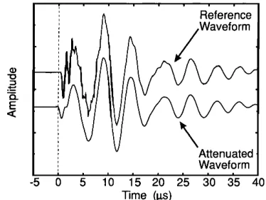
FIG. 1. Two waveforms, with and without effects of attenuation, are shown

in the upper plot. The reference waveform arrives at time tl, while the atten- uated waveform arrives a time interval t s, earlier indicative of higher veloc- ities in the dissipative media. The unattenuated waveform is taken as the reference waveform. The spectra of the two are computed and compared in

lower frame. The relative rolloff of the attenuated waveforms is used to cal-

culate the attenuation in the spectral ratio method.

proach, an attenuated waveform is windowed and the time

series is transformed into the spectral domain with an FFT

(Fig. 1 ). An estimate of an unattenuated waveform is ob-

tained by calibrating transmitter-receiver pairs in a nondis-

sipative medium, or by assuming that the source characteris-

tics are known.

A

Let Wc (fn) be a magnitude of the amplitude spectrum

of an unattenuated waveform (the reference waveform) at A

each discrete frequencyfn of the transform, and let W(f, ) be

the estimate of the attenuated waveform. If the waveforms

have traversed a distance •Sx, then the estimate of attenu-

ation a(f) is given by

A A

-- In [ W(f, )/Wc (f,) ]

a(f•) = (4a)

•x

or

ln[ Wc

(xn)] - ln[ W(f, )]

a(fn) = . (4b)

•x

A least-squares line is fit to values of log(a) plotted against

frequency; the values of k and N are derived from the inter-

cept and slope of the fit, respectively. This technique is called

the spectral

difference

or the spectral

ratio method.

2ø'2•

Although this approach is simple and straightforward,

difficulties arise when multiple arrivals of the transmitted

energy fall within the selected sampling window. This effect

has been shown to be a significant and sometimes dominant

effect on estimates of attenuation derived from seismic re- flection data. 22-24 Unfortunately, single arrivals cannot al-

ways be separated or isolated; bandlimited energy necessar-

ily arrives in wave packets of finite length that may overlap

following events. The frequency content of the waveform

(or, equally, the wave packet width) determines the mini-

mum duration of the sampling window if one wishes'to re-

solve spectral peaks and reduce effects of spectral sidelobe

leakage. 25 If a window brackets less than several cycles of

the dominant frequency in the waveform, then Fourier transform estimates of spectral energy are less accurate.

Thus both the window size and presence of secondary arri-

vals place strong constraints on the applicability of the FFT

spectral difference method. These effects are illustrated in

Sec. III.

II. FILTER-CORRELATION METHOD

The filter-correlation method is a two-stage procedure

that can give superior estimates of attenuation when length

of time windows must be reduced to minimize the effects of

secondary multipath arrivals. Assume that two waveforms

are available for analysis, an unattenuated reference wave-

form wC(t) and an attenuated waveform w(t), where t is

time (Fig. 2). The waveforms have been sampled N times at

equal intervals tSt, in a window of length T = NtSt. The value of w(t) at a specific time ktSt is denoted by wk; k = 1,N.

The waveforms in Fig. 2 were derived from measured signals collected in the lab. The reference waveform was tak- en from a digitized signal transmitted between a pair of pie-

zoelectric transducers inserted in distilled water. The atten-

uated waveform was generated by applying a

pseudoattenuation filter [ Eqs. ( 1 ) and (2) ] to the reference.

The waveforms contain two spectral power peaks near 200

and 800 kHz, corresponding to longitudinal and radial reso-

nant oscillations of the crystal transducers. The data were

sampled at a rate of 20 MHz and most of the energy in the

waveform lies between 100 and 1200 kHz. The oversampling in time relative to the Nyquist criterion allows an accurate temporal resolution in the following correlation step. This

Reference .Waveform

Attenuated Waveform

-5 0 5 10 15 20 25 30 35 40

Time (its)

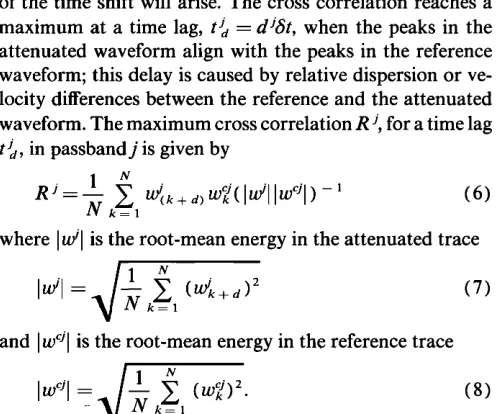
FIG. 2. The test reference waveform and the filtered attenuated waveform

are plotted for an attenuation of k = 2.0 X 10 - 3 and N = 1.7 giving an at-

tenuation. a -- 252 dB/m at 1000 kHz. The attenuated pulse was assumed to

have traveled tSx = 0.07 m.

temporal resolution ultimately determines the resolution of velocity dispersion.

The first arrival of energy in the reference waveform occurs at time t• (Fig. 1); in practice the position of first arrival is determined with a simple threshold criterion. The attenuated waveform has traveled a distance 5x through a dissipative media. The first arrival of energy in the attenuat- ed waveform is aligned with that of the reference waveform by applying a time shift ts. This time shift gives the prelimi-

nary estimate of the velocity of the media, Vo = •x/(t•- ts). Both reference and attenuated wave- forms may contain secondary reflections from the boundar-

ies of the measurement apparatus. A subjective choice is

made to choose a window that excludes these secondary arri-

vals. Other criteria for choosing the window size will be dis-

cussed in subsequent sections.

The first step of the method applies a series of causal bandpass filters to the entire recorded length of the reference

and attenuated waveforms. A causal filter is used to prevent

the migration of energy of secondary arrivals backward in

the filtered time series. Noncausal filters, such as a zero

phase filter, would allow contaminant energy to leak back into windows used for waveform comparison.

This procedure is applied for a number of discrete pass-

bands for which significant energy is present in the wave-

form; the number of frequency bands, n band, is usually cho-

sen to range from four to eight. The choice of the number of

passbands and the width of each passband is somewhat arbi-

trary and is based on the characteristics of the waveforms

under study. The filtered estimate of the attenuated data w j in passband j is given by

M

WJk

-- • gJmW(m_k)

,

(5)

m--1

where gtm are the passband filter coefficients of total length M. The filtered calibration data W c• are generated in the

same way.

In this paper, an eight-pole causal Butterworth filter

routine modified from Kanasewich 26 was used to generate

the filter coefficients. This filter has a dropoff of 3 dB at the

bandpass limits and a rolloff of 48 dB/decade. Other causal

filters could be used in this stage although no comparison

between filter types has been made by the authors.

The result of the first stage of the process is depicted in

Fig. 3 for six passbands ranging from 300-1100 kHz. The

relative decrease of the amplitude of the attenuated data

with respect to the calibration data shows an increasing at-

tenuation with frequency. The relative offset of the peaks of

the attenuated waveform reveals frequency-dependent ve-

locity differences between the calibration and the attenuated

data in each separate waveband. The change in this offset with frequency is a measure of the velocity dispersion of the

wave.

The second stage of the process entails a cross correla-

tion between the reference and attenuated waveforms in

each of the passbands within the limits of a window of the

filtered time series. No taper is applied to the data, other than the choice of a prearrival and post-arrival time. The filtered attenuated signal is shifted back and forth to align

' ' ' ' ' - ' - 3;0-40(• kHz J

t

400-500 kHz

.R

A

5;0-60(• kHz

J

: : : :

[ ,.. .•llli, lOOO-11oo kHz

5 10 15 20 25 30 35 0 5 10 15 20 25 30 35

Time (ITS) Time (IZS)

FIG. 3. The waveform data in six passbands are plotted after the first stage of the method. The amplitudes of the attenuated waveforms (A) are plotted relative to the reference (R). The progressive decay in relative amplitude with frequency is obvious.

peaks with the reference by up to a maximum of one half- cycle of the mean passband frequency. The cross correlation, if continued outside this limit, would exhibit multiple local maxima offset by the period of the mean frequency of the passband. If the initial alignment of the reference and atten-

uated waveforms is in error by more than this limit, then errors in choosing the correct local maxima for calculation of the time shift will arise. The cross correlation reaches a

maximum at a time lag, t• --d•St, when the peaks in the

attenuated waveform align with the peaks in the reference

waveform; this delay is caused by relative dispersion or ve-

locity differences between the reference and the attenuated

waveform. The maximum cross correlation R •, for a time lag ß

tõ, in passband j is given by

N

5;

Im )-'

(6)

Sk=l

where

I•l is the root-mean

energy

in the attenuated

trace

i•_

1 • (•k+a

(7)

and I wOl

is the root-mean

energy

in the reference

trace

(w7)

(8)

The cross-correlation process is used to align attenuated

waveform data with the reference waveform. Once aligned,

estimates of amplitude differences caused by attenuation can

be easily made.

Estimates of the mean frequency in each passband are

calculated by averaging the mean of the zero crossings of the

filtered waveforms. If •t• is the mean time between zero

crossings in the waveform after the time of first arrival of

coherent energy in each passband, then the mean frequency

of the attenuated waveform is defined as

f•m = (25t•) --1 (9)

. ^ ^ 3oo-4o6 mz /

'R

'A

: . : , , , ,

, R II.. 500-600 kHz/

'R

... ! , J , J , • ,

0 5 10 15 20 25 30 35

Time (gs)

... 8•o-goo' '

,

'R

, I• •, 1000-1100 kHz ,

ß R

0 5 10 "•)' 20 25 30 35

Time (Izs)

FIG. 4. The waveform data in six passbands are plotted after the cross- correlation stage. The time shifts and calculated amplitude ratios have been applied to the attenuated waveforms in order to display maximal cross cor-

relation with the reference waveforms. This misfit between the reference

and attenuated waveforms is small; the correlation value (see text) exceeds

0.99 for each set.

•. 1000

J

Applied

Attenuation

E lOO/[]

....

[] Filter

• Correlation •

•

T

• ....

• Spectral

Difference

• lO

6 izs window

11

• 1øøø

/

E •ooT

v

11

C•

X

22

IZS

windoK

1 O0 1000

Frequency (kHz)

FIG. 5. Attenuation estimates of the filter-correlation method (square sym- bol) and the spectral ratio method (triangle) are plotted as a function of frequency. The solid straight line is the target attenuation.

and similarlyf• for the reference waveform. Other methods

were tested to estimate the mean frequency (e.g., average of

the passband limits, maximum entropy analysis, cross-cor-

relation techniques) but the zero crossing method proved

most simple, most reliable and most accurate.

In Fig. 4, the reference and attenuated waveforms are

plotted in each passband after the correlation stage where

relative time shifts and mean energies have been calculated.

The waveforms are normalized by their root-mean energy

and the attenuated data shifted by t•. This figure shows that

the filter-correlation method essentially performs a wave-

form fitting in each of the passbands, extracting information

about time delay and amplitudes in each discrete frequency

band.

Estimates of frequency-dependent velocity v • in each

pass band are calculated using the time delay offsets and the preliminary time shifts

•x

d= . . (10)

t/--t• +tõ

Estimates of the attenuation a( in each passband are given

by

aj = -- ln(

lu•l/lwcJ

I ).

( ] ])

&x

The calculation of k and N in Eq. (2) is made by a least-

squares fit straight line between log(a J) against the average

between the mean frequencies in the attenuated and refer-

ence passbands, as shown in Fig. 5.

Ill. COMPARISON WITH THE SPECTRAL METHOD USING SYNTHETIC DATA

A series of comparisons between the filter-correlation

method and the spectral difference method were made on

synthetic

data

shown

in Fig. 2. Results

for two

different

sets

of trials are reported here. The first series compares results of

the two methods as a function of the size of the data window.

The second series contrasts predictions for an attenuated

waveform that contains a secondary multiple arrival. These

comparisons serve to illustrate the effectiveness of the filter-

correlation method.

In both cases the attenuated wave was filtered with the following attenuation parameters: k = 0.0174 dB/m-kHz •v

and N = 1.7. The distance traveled by the attenuated wave

•Sx was set to 0.0715 cm. These values correspond to a net

attenuation of 252 dB/m at 1000 kHz. A progressive phase

shift was applied to induce a linear increase of velocity by 10

m/s from 100 to 1000 kHz.

For calculation of FFT estimates, waveforms within the

comparison window were multiplied by a Welsh window. 25

The Welsh window applies the weighting operator,

«(N•+I) '; j=l, Ns,

over the length of the window Ns. The choice of the window type affects the results of the spectral difference method,

underlining the inherent difficulties with this approach.

FFT spectral estimates between 100 to 350 kHz and 650

to 1000 kHz were used to compute attenuation parameters in

the spectral difference method, avoiding a notch in the pow-

er spectra at 500 kHz. Eight passbands were used in the

filter-correlation method: 300 to 400 kHz, 400 to 500 kHz, 500 to 600 kHz, 600 to 700 kHz, 700 to 800 kHz, 800 to 900 kHz, 900 to 1000 kHz, and 1000 to 1100 kHz.

In the first test series effects of window length are tested.

The comparison window was chosen with a fixed pre-arrival

interval of 4/•s with a variable period of 5 to 25/•s after the first break of coherent energy. Estimates of attenuation ver-

sus frequency were generated and estimates of k and N were

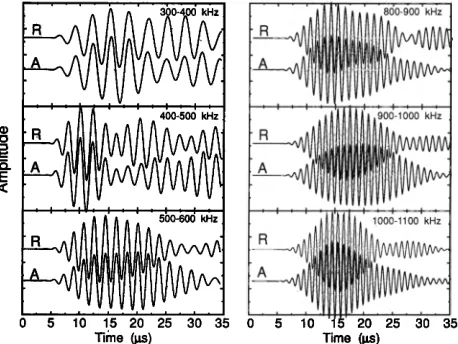
derived from a least-squares fit to the data. The results are

plotted in Fig. 6; estimates of a at 1000 kHz and N are given

as a function of the the sum of the pre- and post-arrival win- dow lengths.

300[

250

I

200[

150• 2.0

1.5

1,0 0

• []

a

Spectral

Differen•cE

10 20 30

Combined Window Length (ps)

FIG. 6. The estimates of a and Nat 1000 kHz are plotted as a function of the post-arrival window size. The filter-correlation estimates are marked by the triangle symbol, while the spectral difference (FFT) estimates are marked by the square symbols.

The filter-correlation method produces superior esti-

mates of a and N. The spectral difference method seriously

underestimates a for window sizes less than 18 •ts; errors

approach 50% of the target value in the worst case. At least

25 •ts of uncorrupted data are needed to make good estimates

of the attenuation parameters using the FFT method, while a

window of 15 suffices for the filter-correlation method. FFT- derived estimates of iV show considerable error and no confi-

dence can be placed in results produced by this method.

A second series of tests were made with a secondary

multiple that arrives 10 •ts after the first arrival of coherent energy. The amplitude of the multiple was set to -- 0.5 times

that of the attenuated wave in Fig. 2. The multiple waveform

and the reference waveform are shown in Fig. 7. The effects

of the secondary multiple are seen in the later part of the

waveforms.

The predictions of a and N for the second test series are depicted in Fig. 8. The filter correlation method continues to make better estimates of a until 20•ts, well after the arrival of

the secondary multiple. The estimate of iv progressively but

uniformly degrades, erring by -- 8% at 22 •ts. The spectral

difference method fails to make a comparable estimate of

these acoustic parameters and at no time produces accepta-

ble results. By 23 •ts, the estimate of N is 25% below that

applied.

These tests of synthetic data confirm the stability and accuracy of the filter-correlation method using short win- dow lengths in the presence of a secondary multiple. Al-

though the multiple problem is not completely removed, the

effects of the multiple on the results predicted by the filter- correlation method are greatly reduced. The spectral differ-

ence method results in more variable estimates of the acous-

tic parameters as the length of the time window changes; a

meaningful value based on these estimates would be hard to

constrain.

IV. APPLICATION TO FIELD DATA

In the spring of 1987, a set of compressional wave data

was collected on large diameter ( 11.4 cm) piston cores taken

ß , ß ' [ ' ' ' Reference

•

Attenuated

I Secondary

Arrival

Wavef,orm

i , i at 1,0 j. ts , , ,

-5 0 5 10 15 20 25 30 35 40

Time (•s)

FIG. 7. The attenuated waveform has been augmented by a secondary arriv- al at 10/rs after the time of the first arrival of energy. The secondary arrival has an amplitude of -- 0.5 times the attenuated waveform in Fig. 2.

from Emerald Basin, a Quaternary deposit of unconsolidat-

ed glaciomarine clay and silts located approximately 100 km

south-southeast of Halifax, Nova Scotia. 27 Piston cores

were split normally within 24 h of collection, and acoustic

properties were measured immediately thereafter. Biogenic

gas caused expansion and cracking of some of the cores.

Acoustic measurements made on these cores showed a sig-

nificant reduction in the amplitude of transmitted sound and

these measurements were discarded. In situ measurements 28

might avoid this problem; however, velocity measurements

at more than one direction to the bedding plane would be difficult with a remotely deployed device. A more complete

discussion of the data collection and analysis of these data

are the subject of another paper; 29 only a sample of wave- form data from core 87003-004 is discussed here.

Compressional wave data were collected using a marine sediment acoustic measurement system as described by

Baldwin. 3ø The system was modified by the authors, incor-

porating digital recording, automatic first break detection,

and processing of the acoustic waveform data. The system

uses two pairs of piezoelectric transducers of small diameter

300

200

lOO 2.0

z 1.5

1.0 0

[] Spectral Difference

• Filter Correlation @ lOOO kHz

, ,

10 20 30

Combined Window Length (Izs)

FIG. 8. Estimates of a and Nat 1000 kHz as a function of window size for

the case of the secondary multiple given in Fig. 7. The spectral difference (FFT) estimates are highly sensitive to the presence of the multiple.

(0.635 cm). Each transducer has two major electromechani-

cal resonances near 200 and 800 kHz. The transducers are

potted in aluminum probes that can be inserted directly into

the split piston core with minimal disturbance of the sedi-

ment. Each pair of probes forms a source and receiver com- bination. A high-voltage, short-duration (2/is) pulse is ap- plied to the transmitter and the time of flight of the transmitted energy to the receiver is used to estimate the sediment velocity. The received waveform is digitized and

stored on disk.

The geometry of the two set of probes is rigidly fixed. One set of probes is aligned along the axis of the piston core

and has a transducer separation of 0.07 m. The other pair is

aligned transverse to the core axis and has a separation of

0.045 m. The separation between the transmitter and receiv-

er pair is calibrated in distilled water. The temperature of the distilled water and the sediment is continuously recorded

during the measurement. The waveform passed through the

distilled water is used as the reference waveform, making

corrections for waveform geometrical spreading unneces-

sary. In these measurements, sediment velocities and attenu-

ation values are computed relative to that of distilled water, a

known standard.

Time (l•S)

40 50 60 70 80

0 ... I .... I .... I ... -

4 _

8

12

16

•' •/' - •/ ,a• •

>• 2

,

4

• 6

n' 8 ....

/•

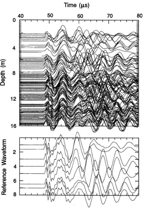
FIG. 9. The top diagram shows waveform data taken through clay/slit sedi- ments from Emerald Basin, while the lower diagram shows calibration waveforms collected in distilled water. Both data sets show coherency in the first 10 fts between adjacent waveforms after the first arrival of energy. The arrival of secondary reflections and other multiples mask coherency later on

in the time series.

Preliminary estimates of the first arrival of energy are

made automatically using a simple amplitude threshold cri- terion; the operator has the option to manually reposition

the first break position, although it was not necessary with

these data. Measurements of velocity were made every 10 to

20 cm down the core, over a distance of up to 20 m.

Waveform data for the longitudinal measurements are

illustrated in Fig. 9, with with eight waveforms of water cali-

brations.

A visual

inspection

indicates

that the waveforms

are highly correlated for the first 10/is after the first arrival of energy. After that time, a train of uncorrelated phases

arrive at random times.

These secondary arrivals arise from reflection off the

top, side, and end boundaries of the split core. The amplitude and arrival time of these multipath arrivals depend critically on the precise position of the transducer pair relative to the boundaries of the sediment sample. In practice, small differ-

ences of the transducer positions between successive mea-

surements cannot be avoided. In some cases, the thickness of

the split core varies; in other cases, measurements are made

near the ends of core sections. In a spectral difference meth- od at least 25 fts of the waveform would have to be windowed

to resolve the parameters with any confidence, which would

include significant multipath energy. The filter correlation

method however allows the accurate calculation of the at-

tenuation parameters within the physical constraints of the

data set.

Emerald Basin core data were processed with eight

passbands

(those'listed

in the previous

section)

and

with a

pre-arrival length of 4/is and a post-arrival length of 10

Estimates of velocity a and Nat 1000 kHz are plotted in Fig.

10 for both longitudinal and transverse measurements. Since

the measurement along each direction is independent, in the

absence of significant anisotropy, the results are indicative of

the accuracy and repeatability of the method. At each depth

in Fig. 10, the extreme excursions of the error bars indicate

the longitudinal and transverse measurements, while the

Velocity N

(m/s)

1425 1450 1475 1500 0 I 2

0 .... ! .... , ... • .... , ....

(dB/m)

250 500 0

.... , ....

ß

@ 1 MHz •

FIG. 10. Estimates of velocity a and N at 1000 kHz are plotted for core 87003-004. The solid line plots the mean between the transverse and longi- tudinal measurements and the error bars mark excursion of the longitudinal and transverse measurements from the mean.

center of the error bar plots the average value. The values of velocity have been corrected to a temperature of 10 øC.

The values of velocity are most highly constrained. The

transverse and longitudinal measurements generally agree

within 5 m/s. The estimates of attenuation show more rela-

tive scatter, but the most agree within 10% at 1000 kHz. The

estimates of N average around 1.5 and show an average dif-

ference of less than 0.15. These sediments thus show a mar-

kedly nonconstant Q and have high values of N that are in

good agreement with those predicted by Biot-Stoll theory. 3•

The passband estimates of velocity at 1000 kHz were

uniformly lower than the preliminary estimates based on the

first arrival of energy. The average difference between the

velocity estimate for the lowest band (300 to 400 kHz) and

the time of flight estimate was -- 12.6 + 2.5 m/s. The aver- age difference between the velocity in the lowest passband

(300 to 400 kHz) and the highest passband (1000 to 1100 kHz) was -- 2.9 + 1.4 m/s, weakly resolved in this analysis. The smallest difference between velocity estimates is 1.5 m/s, determined by the transducer separation and digitiza-

tion rate. These data indicate that, although dispersion is not important between 300 and 1100 kHz, the use of first break estimates of the waveform can significantly bias velocity esti- mates. This effect may be attributed to the arrival of higher frequency energy above the passbands.

Although a detailed discussion of this data set is present-

ed elsewhere, 29 the acoustic data present new and useful in-

formation about the cored sediment. The velocity data

shows a marked increase at 11-m depth. This change corre-

lates with a pronounced change in the character of high- frequency seismic reflectors, and marks a transition from the

proglacial Emerald Silt unit to the transgressive LaHave

Clay unit. 27 The transition was not obvious from a visual

inspection of the split core.

v. ANISOTROPY

X-ray photographs of these sediments reveal microscale

banding, interpreted as thin layers of sand intercalcated with

Porosity

0.4 0.5 0.6 0.7 0.8 0.9 -2 0 2

0 / '•

5

15 I '

20 ...

Velocity Anisotropy Attenuation Anisotropy (m/s) (dB/m)

4 6 8 -20 -10 0 0

i i i i i

FIG. 11. Porosity is plotted against depth in the core. The anisotropy (the difference between transverse and longitudinal measurements) in both ve- locity and anisotropy is plotted in the center and right-hand frames. A five- point median filter was applied to both anistropy plots before plotting to reduce scatter, highlighting changing trends in these measurements.

clay and silt on a subcentimetre scale. It has been predict-

ed

32'33

that a finely layered

media should

show compres-

sional wave anisotropy, induced by shear coupling between

adjacent layers.

In Fig. 11 the velocity anisotropy, expressed here as the difference between the transverse and longitudinal veloc- ities, is plotted against depth in the core. Porosity, derived

from bulk density measurements, and the anisotropy in at-

tenuation in the core are also plotted. The velocity anisotro-

py increases progressively with depth toward a value of 6

m/s at 16 m, punctuated by a significant negative excursion

of --2 m/s near 11 m. The negative excursion correlates with a sharp increase in the mean velocity (Fig. 10). The velocity anisotropy increase appears to correlate inversely

with the porosity, although the regression between the two

variables has a low correlation value of less than 0.5. No

consistent trend in the attenuation anisotropy is observed,

although the transverse attenuation is generally lower than

the longitudinal measurement.

We use a simple two-layer model to investigate the ob-

served anisotropy. Following Brekhovskikh, 32 the compres-

sional wave velocity czz for waves propagating perpendicular

(corresponding to the longitudinal measurement axis) to the layering is given by

c

2 =

2

(13)

p[ 1/(2, + 2/z2 ) + 1/(,t2 + 2/z2 )]

Here .;[•,/t•,/t. 2 , and/t 2 are the Lam• elastic constants of two, repeatedly interbedded, thin layers of equal thickness. It is assumed that the wavelength of the acoustic waves is

much greater than the layer thicknesses. The mean density

of the two layers is p. The ratio of the compressional velocity %,,, of waves propagating parallel to the layers to c• is

c• 2

(/•2 --/• ) [22 +/•2 -- (;t• +/• ) ]

(•-zz)--1-F

(14)

Levin • gives equivalent formulas using compressional and

shear velocities, but the relationships using the Lam• con-

stants are simpler and show clearly the effects of shear cou-

pling between the layers. For example, no velocity anisotro- py is predicted when the shear moduli of both layers are

equal. Under most circumstances, the ratio is greater than,

or equal to, 1 for structurally competent sediments, and the

transversely measured velocity should exceed the longitudi-

nal measurement. The numerator of the second term of Eq.

(14) can be negative, resulting in a velocity ratio less than 1,

when

(tt: - tt, ) [2: + tt: - (2, + tt, ) ] < 0.

This condition may be met as the Poisson's ratio •r of one of

the layers approaches that of a fluid 33 (•r = 0.5 ).

Values of the Lam• parameters for the Emerald Basin

sediments must be obtained through inference based on em-

pirical data. Hamilton 34 derived parametrized estimates for

the frame modulus of marine sediments from experimental

data. His data are referenced to an overburden pressure of 1

m or less, appropriate for split core data as presented here.

Using Hamilton's expression for natural silty clays, the

shear modulus as a function of porosity • is given by

ft (•) 3

( 1 -- 20-)e

2'7350-4'25075•

2(1

where a is set to 0.3.

The variation of the compressional wave velocity with

porosity has been described frequently in the literature; we

will use an expression given by Anderson 35 based on veloc-

ities of sediments found in the depth range 0.1-1.5 km (Ta-

ble 4 of Anderson 35 ) corrected to a temperature of 10 øC: v, (•) = 2478-2724• + 1816• 2. (17)

A least-squares fit of a quadratic through the velocity data

(Fig. 10) plotted against porosity (Fig. 11 ) collected on the

Emerald Basin core yields

vb (•) = 1782-833• + 522•32. (18)

This expression applies within the porosity range of the data

(0.55-0.78); however, its validity at higher and lower poro-

sities must be questioned. Figure 12 plots the observed data

against the two quadratic forms. Anderson's expression pre-

dicts significantly higher increases in velocity outside the

observed porosity range.

Estimates of A are derived from estimates of these veloc-

ities using estimates for the shear modulus and bulk density:

A = [p• + (1 - •),o m

]u2(•) - 2•(•),

(19)

where

the fluid density

p• is 1030

kg/m 3. The density

of the

grainspro of the sediments was measured on the cores, giving

mean value of 2780 kg/m 3.

Although the porosity has been used here to predict the values of the elastic parameters, other factors, including

grain size, grain alignment, grain contact cementation, grain

composition, and consolidation history, will have significant

effects. Given these caveats, only the porosity parametriza-

tion is employed here.

Using these estimates of A and/•, Eqs. (13) and (14)

can be used to predict the velocity difference between trans-

verse and longitudinal measurements as a function of poros-

1700 ...

1600

15OO

1400 0.4

+++ +

I Vh:

1782-833•

+552

(I)

2

0.5 0.6 0.7 0.8 0.9 Porosity

FIG. 12. The upper curve plots the parametrization of velocity by porosity

35

given by Anderson; the lower curve is the best-fit quadratic to porosity and velocity values (marked by crosses) measured in the Emerald Basin

cores.

ity. The abscissa in Fig. 13 (a) is the mean porosity of the two

layers, that which would be obtained from bulk measure-

ments. The vertical axis measures the porosity in the layers

of the model. A vertical line drawn at a specified value of the

mean porosity intersects an anisotropy contour of a chosen

value twice; the vertical coordinates at these intersections

define a pair of layer porosities which would induce an ani-

sotropy of the value of the specified contour. For example, a

vertical line drawn at a mean porosity of 0.65 intersects the

5-m/s contour at layer porosities equal to 0.45 and 0.85 (the

mean of the two is, of course, 0.65). Contours are restricted

to an area of the plot where the layer porosities are greater

than 0 and less than 1.

Figure 13(a) shows that above a porosity of 0.75, the

calculated anisotropy does exceed 5 m/s; the magnitudes of

the shear modulus are too small at these high porosities to

have much effect. As the mean porosity falls, the shear mod-

ulus increases and larger values of anisotropy can be pro-

duced. Near a porosity of 0.5, a wider range of anisotropy

values can be produced, up to 80 m/s. However, for the

largest values, a fluid would have to be interbedded with a

layer having no porosity, a physically untenable circum-

stance for surficial sediments. At a porosity of 0.55, typical of the bottom section of the Emerald Basin core, layer poro-

sities of 0.38 and 0.72 would induce an velocity difference of

6 m/s, close to that observed. These porosities are not unrea- sonable for interbedding of clay and sand layers.

The least-squares fit expression [Eq. (18) ] predicts less anisotropy, although the general shape and trends in con- tours are similar. At a mean porosity of 0.65, layer porosities

of 0.47 and 0.83 would induce a velocity difference of 4 m/s,

roughly 1 m/s less than predicted with Eq. (17). At a poros- ity of 0.55, layer porosities of 0.34 and 0.76 are needed to get a velocity difference of 6 m/s. Again, these porosities are not

unreasonable for interbedding of clay and sand layers. The

least-squares fit expression predicts approximately 80% of

the velocity anisotropy predicted by Anderson's expression.

In summary, the two-layer model can produce velocity

anisotropy values similar to those observed in the Emerald

Basin cores. At the top of the core where porosity ap- proaches 0.80, the model predicts that anisotropy cannot exceed 2 to 3 m/s, in agreement with the observations. As the

mean porosity decreases with depth in the core, the theory

predicts that higher levels of anisotropy can be produced by porosity variations. Layer porosities must vary between

35% and 75% at the bottom of the core to fit the observed

velocity data, consistent with clay and sand interbedding.

The model cannot predict a negative anisotropy as ob- served in the core data. Presumably, the parametrization of

the Lam• elastic constants fails in this region. Perhaps the

cored material had been disturbed by sampling in this re- gion, resulting in weakened and fluidized layers interbedded

with competent layers. No systematic trends in attenuation

anisotropy is observed. Any attempt to model the attenu- ation anisotropy data would likely be overly speculative.

Vl. CONCLUSIONS

This paper has presented the filter-correlation method,

a means of extracting consistent and accurate estimates of

(a)

o.o o.5 1 .o

Mean Porosity

(b) 1.0

13= 0.5

0.0

0.0 O.5 1.0

Mean Porosity

FIG. 13. (a) A contour plot of the difference in velocity for waves propagat- ing parallel and perpendicular to a thinly bedded, two layer model using Anderson's 3s parametrization of velocity by porosity. The horizontal axis is the mean porosity of the two layers and the vertical axis is the layer porosity.

A vertical line at a given value of the mean porosity intersects a contour of a

fixed value twice, corresponding to the porosities of each of the two layers. Velocity contours are 5 m/s. (b) A contour plot of the difference in velocity for waves propagating parallel and perpendicular to a thinly bedded, two- layer model using the least-squares fit quadratic parametrization of velocity

by porosity. Velocity contours are 4 m/s.

acoustic parameters from acoustic waveform data. The

method minimizes problems associated with short time win-

dows, which tend to corrupt attenuation estimates made

with Fourier spectral techniques. The filter-correlation method makes superior estimates in the presence of a multi-

path secondary arrival.

Preliminary analyses of acoustic data collected on cored

marine silts and clays show that the attenuation properties of these materials cannot be described by a constant Q mecha- nism. A Biot-Stoll mechanism is more likely. Estimates of velocity dispersion show that dispersion in the range of fre-

quencies between 300 and 1100 kHz is small. However, the

arrival of higher frequency data biases the estimate of veloc-

ity made by first break detection upward by about 12 m/s.

The filter-correlation method permits the calculation of ve-

locity in a fixed waveband, necessary for accurate modeling of the data.

Accurate estimates are needed to measure compres-

sional wave velocity anisotropy in unconsolidated sedi-

ments. The compressional wave velocity parallel to the bed-

ding plane of the sediments is consistently higher than those of the waves propagating perpendicular to the planes, in-

creasing from 0 m/s at the surface of the core to 6 m/s at 15

m. The error in velocity caused by ignoring this effect is less than 1%. A simple two-layer model suggests that the ob-

served velocity anisotropy is consistent with a decrease in

bulk porosity with depth in the core and small-scale inter-

layering between alternating layers of contrasting porosity.

ACKNOWLEDGMENTS

The authors would like to acknowledge the support of

the U.S. Office of Naval Research (Contract N00014-87-G-

0114) and the Natural Sciences and Engineering Research

Council of Canada. We would like to thank the officers and crew of CSS HUDSON. Kate Moran and Harold Christian

provided geotechnical expertise.

• S. H. Schock, L. R. Leblanc, and L. A. Mayer, "Chirp subbottom profiler

for quantitative sediment analysis," Geophysics 54, 445-450 (1989). 2 M. A. Biot, "Theory of propagation of acoustic waves in a fluid-saturated

porous solid, I. Low frequency range," J. Acoust. Soc. Am. 28, 168-178 (1956).

3 M. A. Biot, "Theory of propagation of acoustic waves in a fluid-saturated porous solid, II. Higher frequency range," J. Acoust. Soc. Am. 28, 179- 191 (1956).

4 M. A. Biot, "Mechanism of deformation and acoustic propagation in po-

rous media," J. Appl. Phys. 33, 1482-1498 (1962).

s M. A. Biot, "Generalized theory of acoustic propagation in porous dissi-

pative media," J. Acoust. Soc. Am. 34, 1254-1264 (1962).

6 E. L. Hamilton, "Sound attenuation as a function of depth in the sea

floor," J. Acoust. Soc. Am. 59, 528-535 (1976).

7 E. L. Hamilton and R. T. Bachman, "Sound velocity and related proper-

ties of marine sediments," J. Acoust. Soc. Am. 72, 1891-1904 (1982).

8 R. D. Stoll, "Acoustic waves in ocean sediments," Geophysics 42, 715-

725 (1977).

9R. D. Stoll, "Experimental studies of attenuation in sediments," J. Acoust. Soc. Am. 66, 1152-1160 (1979).

•o R. D. Stoll, "Theoretical aspects of sound transmission in sediments," J. Acoust. Soc. Am. 68, 1341-1350 (1980).

• R. D. Stoll, "Marine sediment acoustics," J. Acoust. Soc. Am. 77, 1789- 1799 (1985).

•2 S. A. Goss, R. L. Johnston, and F. Dunn, "Compilation of empirical ul-

trasonics properties of mammalian tissue II," J. Acoust. Soc. Am. 68, 93-

108 (1980).

13 S. Shaffer, D. W. Pettibone, J. F. Havlice, and M. Nassi, "Estimation of the slope of the acoustic attenuation coefficient," Ultrason. Imag. 6, 126-

138 (1984).

]4 K. A. Dines and A. C. Kac, "Ultrasonic attenuation tomography of soft

tissues," Ultrason. Imag. 1, 16-33 (1979).

•s A. C. Kibblewhite, "Attenuation of sound in marine sediments: A review with emphasis on new low-frequency data," J. Acoust. Soc. Am. 86, 716- 737 (1989).

16 C. S. Clay and H. Medwin, Acoustical Oceanography: Principles and Ap-

plications (Wiley-Interscience, New York, 1977), pp. 185-187. •7 B. J. Brennan and D. E. Smylie, "Linear viscoelasticity and dispersion in

seismic wave propagation," Rev. Geophys. Space. Phys. 19, 233-246 (1981).

•8 G. T. Kuster and M. N. Toksoz, "Velocity and attenuation of seismic

waves in two-phase media: Part II. Experimental results," Geophysics 39,

607-618 (1974).

•9 M. Badri and H. M. Mooney, "Q measurements from compressional seis-

mic waves in unconsolidated sediments," Geophysics $2, 772-784

(1987).

20 D. Goldberg and B. Zinzer, "P-wave attenuation measurements from lab-

oratory resonance and sonic waveform data," Geophysics 34, 76-81

(1989).

2• M. N. Toksoz, D. H. Johnson, and A. Timur, "Attenuation of seismic waves in dry and saturated rocks, I. Laboratory measurements," Geo- physics 44, 681-690 (1979).

22 S. A. Raikes and R. E. White, "Measurements of earth attenuation from downhole and surface seismic recordings," Geophysic. Prospect. 32, 892-

919 (1984).

23 j. R. Resnick, "Stratigraphic filtering," Pageoph 132, 49-65 (1990). 24 T. W. Spencer, J. R. Sonnad, and T. M. Butler, "Seismic Q•stratigraphy

or dissipation," Geophysics 47, 1 6-24 (1982).

2s W. H. Press, B. P. Flannery, S. A. Teukolsky, and W. T. Vetterling, Nu-

merical Recipes (Cambridge U.P., Cambridge, 1986), pp. 420-429.

26 E. R. Kanasewich, Time Sequence Analysis in Geophysics (University of

Alberta, Edmonton, Canada, 1981 ), pp. 266-277.

27 L. H. King, "Surficial geology of the Halifax-Sable Island map area,"

EMR Marine Sciences, Department of Energy, Mines and Resources, Canada, Paper 1, 16 pp. (1970).

28 A. L. Anderson and L. D. Hampton, "A method for measuring in situ

acoustic properties during sediment coring," in Physics of Sound in Ma- rine Sediments, edited by L. Hampton (Plenum, New York, 1974).

29R. C. Courtney and L. A. Mayer, "Acoustic properties of fine grain sedi-

ments from Emerald Basin: Towards an inversion for physical properties using the Biot-Stoll model," J. Acoust. Soc. Am. (to be published). 30 K. C. Baldwin, B. Celikkol, and A. J. Silva, "Marine sediment acoustic

measurement system," Ocean Eng. 8, 489-496 ( 1981 ).

31R. D. Stoll, Sediment Acoustics (Springer-Verlag, New York, 1989). 32 L. M. Brekhovskikh, Waves in Layered Media (Academic, New York,

1960).

33 F. K. Levin, "Seismic velocities in transversely isotropic media, II," Geo-

physics 45, 3-17 (1980).

34 E. L. Hamilton, "Elastic properties of marine sediments," J. Geophys. Res. 76, 579-604 (1971).

35 R. S. Anderson, "Correlation of physical properties and velocity," in Ref.

28.