Dealing with systematics and setting limits
D. S. Sivia
1St. John’s College, Oxford, UK
Abstract. The analysis of data in particle physics often involves systematic uncertainties, and the results entail the setting of limits on inferred parameters. This paper illustrates the former with a simple example, building on the introduction to the Bayesian approach given in Sivia [1], and offers a novel suggestion for the latter.
1 Introduction
The training in data analysis that most of us are given as undergraduates consists of being taught a collection of disjointed statistical recipes. This is generally unsatisfactory because the prescriptions appear ad hoc by lacking a unifying rationale. While the various tests might individually seem sensible at an intuitive level, the underlying assumptions and approximations are not obvious. It is far from clear, therefore, exactly what question is being addressed by their use.
Although attempts to give guidelines on ‘best practice’ are laudable, the shortcomings above will not be remedied without a programme of education on the fundamental principles of data analysis. To this end, scientists and engineers are increasingly finding that the Bayesian approach to probability theory advocated by mathematical physicists such as Laplace [2], Jeffreys [3] and Jaynes [4] provides the most suitable framework. This viewpoint is outlined in Section 2, an instructive example on dealing with systematic uncertainties given in Section 3 and a novel suggestion for setting limits offered in Section 4; we conclude with Section 5.
2 Bayesian Probability Theory
The origins of the Bayesian approach to probability theory dates back over three hundred years, to people such as the Bernoullis, Bayes and Laplace, and was developed as a tool for reasoning in situations where it is not possible to argue with certainty. This subject is relevant to all of us because it pertains to what we have to do everyday of our lives, both professionally and generally: namely, make inferences based on incomplete and/or unreliable data. In this context, a probability is seen as representing a degree of belief, or a state of knowledge, about something given the information available. For example, the probability of rain in the afternoon, given that there are dark clouds in the morning, is denoted by a number between zero and one, where the two extremes correspond to certainty about the outcome. Since the assessment of rain could easily be very different with additional access to the current weather maps, it means that probabilities are always conditional and that the associated information, assumptions and approximations must be stated clearly.
C
2.1 Manipulating Probabilities
In addition to the convention that probabilities should lie between 0 and 1, there are just two basic rules that they must satisfy:
prob(X|I )+probX|I= 1, (1)
prob(X,Y|I )= prob(X|Y,I )×prob(Y|I ). (2)
Here X and Y are two specific propositions, X denotes that X is false, the vertical bar ‘|’ means ‘given’ (so that all items to the right of this conditioning symbol are taken as being true) and the comma is read as the conjunction ‘and’; I subsumes all the pertinent background information, assumptions and approximations. Equations (1) and (2), known as the sum and product rule respectively, are the same as those found in orthodox or conventional statistics; this later school of thought differs from the Bayesian one in its interpretation of probability, restricting it to apply only to frequencies, which limits its sphere of direct application.
Many other relationships can be derived from Eqs. (1) and (2). Among the most useful are:
prob(X|Y,I )= prob(Y|X,I )×prob(X|I )
prob(Y|I ) , (3)
prob(X|I )= prob(X,Y|I )+probX,Y|I. (4)
Equation (3) is called Bayes’ theorem. Its power lies in the fact that it turns things around with respect to the conditioning symbol: it relates prob(X|Y,I ) to prob(Y|X,I ). Equation (4) is the simplest form
of marginalisation. Its generalisations provide procedures for dealing with nuisance parameters and hypothesis uncertainties.
2.2 Assigning Probabilities
While Eqs. (1) and (2), and their corollaries, specify how probabilities are to be manipulated, the rules for their assignment are less well defined. This is inevitable to some extent as ‘states of knowl-edge’ can take a myriad different forms, often rather vague. Nevertheless, there are some simple but powerful ideas on the issue based on arguments of self-consistency: if two people have the same in-formation then they should assign the same probability. We refer the reader to some recent textbooks for a good discussion of this topic, and for examples of Bayesian analyses in general: Jaynes [4], Sivia [1], MacKay [5] and Gregory [6].
3 Dealing with systematic uncertainties
Scientists often talk about statistical and systematic errors, and accuracy versus precision. From our point-of-view, however, these distinctions seem unnecessary. While the use of the term ‘systematic’ suggests that it’s a type of error that could be reduced through calibration, it is simply a source of uncertainty that has be taken into account just like any other. Rather than discussing it in the abstract, let’s consider a specific example.
Suppose we have N measurements of a quantityμ,{dk}; what can be said about the value ofμ? The
information given is insufficient to address the problem unambiguously and so, as usual, the answer will depend on both the data and the assumptions made in the analysis. With the latter denoted by
I, as earlier, the inference is encapsulated by prob(μ|{dk},I ), or the posterior probability distribution
3.1 The simplest case
Let us begin by making some common assumptions: suppose that the measurements are subject to independent, additive, Gaussian noise of constant magnitudeσ. Then, following Section 2.3 of Sivia [1], the chance of collecting the observed data, when given the values ofμandσ, is specified by the likelihood function
prob({dk}|μ, σ,I ) = N
k=1
prob(dk|μ, σ,I ) =
σ√2π−Nexp
− Q
2σ2
, (5)
where Q is the sum of the squares of the mismatch betweenμand the measurements:
Q =
N
k=1
(dk−μ)2. (6)
For a knownσ, this is related to the posterior PDF forμthrough Bayes’ theorem:
prob(μ|{dk}, σ,I ) ∝ prob({dk}|μ, σ,I )×prob(μ|σ,I ), (7)
where the equality has been replaced by a proportionality due to the omission of the denominator,
prob({dk}|σ,I ) =
prob({dk}|μ, σ,I ) prob(μ|σ,I ) dμ , (8)
which is simply a normalisation term. With a uniform assignment for prob (μ|σ,I ) over a suitably
large range, μminμμmax, to express gross prior ignorance about the value ofμ, Sivia [1] shows
that the posterior PDF of Eq. (7) can be summarized by a Gaussian mean and standard deviation
μ = 1
N N
k=1
dk ± √σ
N . (9)
This is a familiar result, with the best estimate ofμbeing the average of the measurements and its reliability improving with the square-root of the number of data.
3.2 Unknown noise level
Since the value ofσwas not specified in the statement of the problem, the posterior PDF forμof relevance is prob(μ|{dk},I ) rather than the one in Eq. (7). Indeed, it’s important to remember that
even the notion of uniform noise is merely part of our simplifying assumptions. Within this context, the appropriate likelihood function for the analysis is related to that of Eqs. (5) and (6) through marginalisation and the product rule:
prob({dk}|μ,I) =
prob({dk}, σ|μ,I) dσ =
prob({dk}|μ, σ,I ) prob(σ|μ,I ) dσ. (10)
With a Jeffreys’ prior for σ, prob(σ|μ,I )∝1/σ, which is uniform with respect to logσto express ignorance about the ‘scale’ parameter, Section 8.2 of Sivia [1] shows that Eq. (10) reduces to
The resultant posterior PDF forμ,
prob(μ|{dk},I ) ∝ prob({dk}|μ,I )×prob(μ|I ), (12)
with a uniform assignment for prob(μ|I ) as before, is found to be approximated well by a Gaussian
for moderately large N (>10 say):
μ ≈μo ±
S
√
N where μo =
1
N N
k=1
dk and S2=
1
N−1
N
k=1
(dk−μo)2 (13)
This is just like Eq. (9), except that the previously given value ofσhas been replaced with an estimate obtained from the scatter of the data.
3.3 Partially known offset
Now suppose that all the measurements are subject to an offsetβ, known from calibration experiments to an extent characterised by prob(β|I ), so that the empirical estimates ofμare ˆdkwhere
ˆ
dk=dk−β . (14)
We are still after prob(μ|{dk},I ), of course, but the related likelihood function entails another nuisance
parameter,β, that needs to be marginalised out:
prob({dk}|μ,I ) =
prob({dk}, β|μ,I ) dβ =
prob({dk}|μ, β,I ) prob(β|μ,I) dβ , (15)
where the likelihood of the data conditional on being givenβ, prob ({dk}|μ, β,I ), is the same as in Eq.
(11) but the formula for Q is modified slightly to
Q =
N
k=1
(dk−β−μ)2. (16)
Ifβis known to beβoto within a standard deviation accuracy of, so that
prob(β|μ,I ) = prob(β|I ) = √2π−1exp
−(β−βo)2
22
, (17)
and N is sufficiently large for the Gaussian approximation of Eq. (13) to be valid, then the best estimate ofμand its reliability yielded by the integral of Eq. (15) is found to be
μ ≈μo−βo ±
S2 N +
2. (18)
The calibration of the systematic offset can be considered adequate if2S2/N, but would benefit
4 Summarizing the inference
4.1 Gaussian-like posterior PDFs
Although the (marginal) posterior PDF for a parameter, x say, encodes our inference about its value, given the data{dk}and the relevant background information I, we often wish to summarize it with just
two numbers: the best estimate of x, xo, and a measure of its reliability,σx. The usefulness of such a
summary, x=xo±σx, relies on the posterior PDF being approximated well by a Gaussian:
prob(x|{dk},I ) ≈
σx
√
2π−1exp
−( x−xo)2
2σ2 x
. (19)
If that is the case, then xoandσxcan either be estimated from the mean and standard deviation of the
posterior PDF,
xo=
x prob(x|{dk},I ) d x and σx2 =
( x−xo)2 prob(x|{dk},I ) d x, (20)
or from the location of its maximum and the curvature at that point,
dL dx
x
o
= 0 and σx−2 = −
d2L
d x2
x
o
(21)
where L=logeprob(x|{dk},I )
. The two estimates will converge if Eq. (19) holds exactly, but should be fairly close as along as the approximation is reasonable.
4.2 Asymmetric posterior PDFs
The above prescription provides a poor summary of posterior PDFs that are highly skew with respect to their modes, because the concept of an error-bar implicitly entails the idea of symmetry: x=xo±σx.
A good way of expressing the reliability with which a parameter can be inferred in such instances is through a confidence, or ‘credible’, interval. Since the area under the posterior PDF between x1and x2is proportional to how much we believe that x lies in that range, the shortest interval that encloses
95% of the area represents a sensible measure of the uncertainty of the estimate:
prob( x1x<x2|{data},I )= x2
x1
prob(x|{data},I ) d x ≈ 0.95 (22)
where the difference x2−x1is as small as possible. The region x1x<x2is called the shortest 95%
confidence interval.
There is no reason why we cannot give the shortest 70%, 99% or any other confidence interval, of course, instead of the conventional 95% one. Indeed, there is something to be said for listing a set of nested intervals since this provides a more complete picture of the reliability analysis; by doing so, however, we are merely reconstructing the posterior PDF!
4.3 Limit-type posterior PDFs
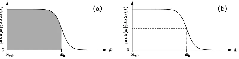
If the posterior PDF is of the form shown in the idealised Fig. 1(a), then we are only able to infer an upper bound for x, xb. Its value is often specified by using the concept of the shortest 95% confidence
interval:
prob( xxb|{data},I )= xb
xmin
Figure 1. An idealised limit-type posterior PDF. (a) The upper bound is traditionally set through the use a shortest confidence interval; (b) the new suggestion is based on the value of the probability relative to its maximum.
where xminis set by the lower bound of the prior PDF for x. The problem with this prescription is that
the resultant xbdepends on xminwhereas the inference about the upper bound is actually defined by the
transition from high to low probability. If the posterior PDF was a step function, for example, then xb
should be at the location of the discontinuity and independent of xmin; neither holds from Eq. (23). A
better way of capturing the nature of the limit-type posterior PDF would be through the specification of xbas the point at which the probability of x drops to a certain fraction of the maximum value:
prob(x|{data},I )
prob(x|{data},I )max
⎧⎪⎪ ⎨
⎪⎪⎩ ><11−−ββ for xfor x<>xxbb (24)
where 0< β <1 defines the level of the significance. That is to say, assuming ideal monotonic decay,
xb→xminasβ→0 and xb→xmaxasβ→100%; xbwould also converge on the discontinuity of a sharp
transition, for allβ, as seems desirable.
4.4 Multimodal posterior PDFs
Depending on the nature of the experimental data to be analysed, posterior PDFs can be multimodal. If one of the maxima is very much larger than the others, the prescriptions of Sections 4.1 and 4.2 may be employed in the neighbourhood of the global maximum. Otherwise, the posterior PDF, and hence our inference about the parameter x, simply cannot be summarized in a meaningful way with just a couple of numbers.
5 Conclusions
The Bayesian viewpoint expounded here follows the approach of mathematical physicists such as Laplace[2], Jeffreys[3] and Jaynes[4], and is still not widely taught to science and engineering un-dergraduates today. It differs markedly in its accessibility for scientists from the works of many statisticians engaged in the Bayesian field; the latter carry over much of the vocabulary and mind-set of their classical frequentist training, which we believe to be neither necessary nor helpful. We refer the reader to some recent textbooks, such as Jaynes[4], Sivia[1], MacKay[5] and Gregory[6], for a good introduction to our viewpoint.
as a crucial number requires some qualified justification. We believe that an understanding of the principles underlying data analysis, along the lines outlined here, is at least as important as formal prescriptions of best practice.
References
[1] D.S. Sivia, Data Analysis — a Bayesian tutorial (Oxford University Press, 1996); 2nd edition with J. Skilling (2006).
[2] P. S. de Laplace, Théorie analytique des probabilités, Courcier Imprimeur, Paris (1812). [3] H. Jeffreys, Theory of probability (Clarendon Press, Oxford, 1939).
[4] E. T. Jaynes, Probability theory: the logic of science, edited by G. L. Bretthorst (Cambridge University Press, 2003).
[5] D. J. C. MacKay Information Theory, Inference, and Learning Algorithms (Cambridge University Press, 2003).