Boosted Decision Trees and Applications

(1)

Boosted Decision Trees and Applications

Yann COADOU

1_{CPPM, Aix-Marseille UniversitNRS/IN2P3, Marseille, France}

Abstract. Decision trees are a machine learning technique more and more commonly

used in high energy physics, while it has been widely used in the social sciences. After introducing the concepts of decision trees, this article focuses on its application in particle physics.

1 Introduction

Decision trees are a machine learning technique more and more commonly used in high energy physics, while it has been widely used in the social sciences. It was first developed in the context of data mining and pattern recognition, and gained momentum in various fields, including medical diagnostic, insurance and loan screening, and optical character recognition (OCR) of handwritten text.

It was developed and formalised by Breiman et al. [ 1] who proposed the CART algorithm (Clas-sification And Regression Trees) with a complete and functional implementation of decision trees.

The basic principle is rather simple: it consists in extending a simple cut-based analysis into a multivariate technique by continuing to analyse events that fail a particular criterion. Many, if not most, events do not have all characteristics of either signal or background. If that were the case then an analysis with a few criteria would allow to easily extract the signal. The concept of a decision tree is therefore to not reject right away events that fail a criterion, and instead to check whether other criteria may help to classify these events properly.

In principle a decision tree can deal with multiple output classes, each branch splitting in many subbranches. In these proceedings only binary trees will be considered, with only two possible classes: signal and background.

Section 2 describes how a decision tree is constructed and what parameters can influence its de-velopment. Section 3 provides some insights into some of the intrinsic limitations of a decision tree and how to address some of them. One possible extension of decision trees, boosting, is introduced in Section 4, and other techniques trying to reach the same goal as boosting are presented in Section 5. Conclusions are summarised in Section 6 and references to available decision tree software are given in Section 7.

While starting with this powerful multivariate technique, it is important to remember that before applying it to real data, it is crucial to have a good understanding of the data and of the model used to describe them. Any discrepancy between the data and model will provide an artificial separation that the decision trees will use, misleading the analyser. The hard part (and interest) of the analysis is in building the proper model, not in extracting the signal. But once this is properly done, decision trees provide a very powerful tool to increase the significance of any analysis.

C

Owned by the authors, published by EDP Sciences, 2013

(2)

2 Growing a tree

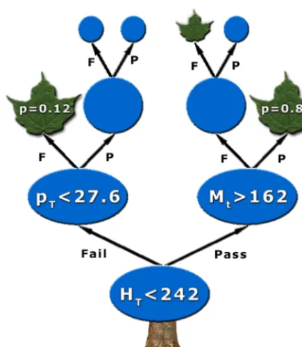
Mathematically, decision trees are rooted binary trees (as only trees with two classes, signal and background, are considered). An example is shown in Fig. 1. A decision tree starts from an initial node, the root node. Each node can be recursively split into two daughters or branches, until some stopping condition is reached. The diﬀerent aspects of the process leading to a full tree, indiﬀerently referred to as growing, training, building or learning, are described in the following sections.

2.1 Algorithm

Consider a sample of signal (si) and background (bj) events, each with weightw_isandwbj, respectively,

described by a setxiof variables. This sample constitutes the root node of a new decision tree.

Starting from this root node, the algorithm proceeds as follows:

1. If the node satisfies any stopping criterion, declare it as terminal (that is, a leaf) and exit the algorithm.

2. Sort all events according to each variable inx.

3. For each variable, find the splitting value that gives the best separation between two children, one with mostly signal events, the other with mostly background events (see Section 2.4 for details). If the separation cannot be improved by any splitting, turn the node into a leaf and exit the algorithm.

4. Select the variable and splitting value leading to the best separation and split the node in two new nodes (branches), one containing events that fail the criterion and one with events that satisfy it.

5. Apply recursively from step 1 on each node.

At each node, all variables can be considered, even if they have been used in a previous iteration: this allows to find intervals of interest in a particular variable, instead of limiting oneself to using each variable only once.

It should be noted that a decision tree is human readable: one can trace exactly which criteria an event satisfied in order to reach a particular leaf. It is therefore possible to interpret a tree in terms, e.g., of physics, defining selection rules, rather than only as a mathematical object.

In order to make the whole procedure clearer, let us take the tree in Fig. 1 as an example. Consider that all events are described by three variables: the transverse momentum, pT, of the leading jet, the

reconstructed top quark mass Mtand the scalar sum of pT’s of all reconstructed objects in the event,

HT. All signal and background events make up the root node.

Following the above algorithm one should first sort all events according to each variable: • ps1

T ≤p

b34

T ≤ · · · ≤p

b2

T ≤p

s12

T ,

• Hb5

T ≤H

b3

T ≤ · · · ≤H

s67

T ≤H

s43

T ,

• Mb6

t ≤M

s8

t ≤ · · · ≤M

s12

t ≤M

b9

t ,

where superscript si(bj) represents signal (background) event i ( j). Using some measure of separation

one may find that the best splitting for each variable is (arbitrary unit): • pT <56 GeV, separation=3,

(3)

Figure 1.Graphical representation of a de-cision tree. Blue ellipses and disks are in-ternal nodes with their associated splitting criterion; green leaves are terminal nodes with purity p.

• Mt<105 GeV, separation=0.7.

One would conclude that the best split is to use HT <242 GeV, and would create two new nodes,

the left one with events failing this criterion and the right one with events satisfying it. One can now apply the same algorithm recursively on each of these new nodes. As an example consider the right-hand-side node with events that satisfied HT < 242 GeV. After sorting again all events in this node

according to each of the three variables, it was found that the best criterion was Mt >162 GeV, and

events were split accordingly into two new nodes. This time the right-hand-side node satisfied one of the stopping conditions and was turned into a leaf. From signal and background training events in this leaf, the purity was computed as p=0.82 (see the next Section).

2.2 Decision tree output

The decision tree output for a particular event i is defined by how itsxivariables behave in the tree:

1. Starting from the root node, apply the first criterion onxi.

2. Move to the passing or failing branch depending on the result of the test.

3. Apply the test associated to this node and move left or right in the tree depending on the result of the test.

4. Repeat step 3 until the event ends up in a leaf.

(4)

There are several conventions used for the value attached to a leaf. It can be the purity p= s

s+b

where s (b) is the sum of weights of signal (background) events that ended up in this leaf during training. It is then bound to [0,1], close to 1 for signal and close to 0 for background.

It can also be a binary answer, signal or background (mathematically typically+1 for signal and 0 or−1 for background) depending on whether the purity is above or below a specified critical value (e.g.+1 if p> 1₂and−1 otherwise).

Looking again at the tree in Fig. 1, the leaf with purity p=0.82 would give an output of 0.82, or

+1 as signal if choosing a binary answer with a critical purity of 0.5.

2.3 Tree parameters

The number of parameters of a decision tree is relatively limited. The first one is not specific to deci-sion trees and applies to most techniques requiring training: how to normalise signal and background before starting the training? Conventionally the sums of weights of signal and background events are chosen to be equal, giving the root node a purity of 0.5, that is, an equal mix of signal and background. Other parameters concern the selection of splits. One first needs a list of questions to ask, like “is variable xi<cuti?”, requiring a list of discriminating variables and a way to evaluate the best

separa-tion between signal and background events (the goodness of the split). Both aspects are described in more detail in Sections 2.4 and 2.5.

The splitting has to stop at some point, declaring such nodes as terminal leaves. Conditions to satisfy can include:

• a minimum leaf size. A simple way is to require at least Nmintraining events in each node after

splitting, in order to ensure statistical significance of the purity measurement, with a statistical uncertainty √Nmin. It becomes a little bit more complicated with weighted events, as is normally

the case in high energy physics applications. One may then want to consider using the eﬀective number of events instead:

Neﬀ = N

i=1wi2

N

i₌1w2i

,

for a node with N events associated to weightswi(Neﬀ = N for unweighted events). This would

ensure a proper statistical uncertainty.

• having reached perfect separation (all events in the node belong to the same class). • an insuﬃcient improvement with further splitting.

• a maximal tree depth. One can decide that a tree cannot have more than a certain number of layers (for purely computational reasons or to have like-size trees).

Finally a terminal leaf has to be assigned to a class. This is classically done by labelling the leaf as signal if p>0.5 and background otherwise.

2.4 Splitting a node

The core of a decision tree algorithm resides in how a node is split into two. Consider an impurity measure i(t) for node t, which describes to what extent the node is a mix of signal and background. Desirable features of such a function are that it should be:

• maximal for an equal mix of signal and background (no separation).

(5)

• symmetric in signal and background purities, as isolating background is as valuable as isolating signal.

• strictly concave in order to reward purer nodes. This tends to favour end cuts with one smaller node and one larger node.

A figure of merit can be constructed with this impurity function, as the decrease of impurity for a split S of node t into two children tP(pass) and tF(fail):

Δi(S,t)=i(t)−pP·i(tP)−pF·i(tF),

where pP(pF) is the fraction of events that passed (failed) split S .

The goal is to find the split S∗that maximises the decrease of impurity:

Δi(S∗,t)= max

S∈{splits}Δi(S,t).

It will result in the smallest residual impurity, which minimises the overall tree impurity. Some decision tree applications use an alternative definition of the decrease of impurity [ 2]:

Δi(S,t)=i(t)−minpP·i(tP),pF·i(tF)

_,

which may perform better for, e.g., particle identification.

A stopping condition can be defined using the decrease of impurity: one may decide to not split a node ifΔi(S∗,t) is less than some predefined value. One should nonetheless always be careful when using such early-stopping criteria, as sometimes a seemingly very weak split may allow child nodes to be powerfully split further (see Section 3.1 about pruning).

For signal (background) events with weightswi

s(wib) the purity is defined as:

p=

i∈signalwis

i∈signalwis+

j∈bkgw

j b

.

Simplifying this expression one can write down the signal purity (or simply purity) as ps =p = _s₊s_b

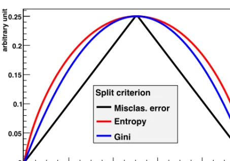
and the background purity as pb = _s₊b_b =1−ps =1−p. Common impurity functions (exhibiting

most of the desired features mentioned previously) are illustrated in Fig. 2: • the misclassification error: 1−max(p,1−p),

• the (cross) entropy [1]:−i=s,bpilog pi,

• the Gini index of diversity.

For a problem with any number of classes, the Gini index [ 3] is defined as:

Gini=

ij

i,j∈{classes}

pipj.

The statistical interpretation is that if one assigns a random object to class i with probability pi, the

probability that it is actually in class j is pjand the Gini index is the probability of misclassification.

In the case of two classes, signal and background, then i=s and j=b, ps =p=1−pband the

Gini index is:

Gini=1−

i=s,b

(6)

signal purity

0 0.2 0.4 0.6 0.8 1

ar

bi

trary un

it

0 0.05 0.1 0.15 0.2 0.25

Split criterion

Misclas. error Entropy

Gini

Figure 2. Various popular impurity

mea-sures as a function of signal purity.

The Gini index is the most popular in decision tree implementations. It typically leads to similar performance to entropy.

Other measures are also used sometimes, which do not satisfy all criteria listed previously but attempt at optimising signal significance, usually relevant in high energy physics applications: • cross section significance:− s2

s+b,

• excess significance:−s_b2.

2.5 Variable selection

As stated before, the data and model have to be in good agreement before starting to use a decision tree (or any other analysis technique). This means that all variables used should be well described. Forgetting this prerequisite will jeopardise the analysis.

Overall decision trees are very resilient to most features associated to variables. They are not too much aﬀected by the “curse of dimensionality”, which forbids the use of too many variables in most multivariate techniques. For decision trees the CPU consumption scales as nN log N with n variables and N training events. It is not uncommon to encounter decision trees using tens or hundreds of variables.

A decision tree is immune to duplicate variables: the sorting of events according to each of them would be identical, leading to the exact same tree. The order in which variables are presented is completely irrelevant: all variables are treated equal. The order of events in the training samples is also irrelevant.

If variables are not discriminating, they will simply be ignored and will not add any noise to the decision tree. The final performance will not be aﬀected, it will only come with some CPU overhead during both training and evaluation.

Decision trees can deal easily with both continuous and discrete variables, simultaneously. Another typical task before applying a multivariate technique is to transform input variables by for instance making them fit in the same range or taking the logarithm to regularise the variable. This is totally unnecessary with decision trees, which are completely insensitive to the replacement of any subset of input variables by (possibly diﬀerent) arbitrary strictly monotone functions of them. The explanation is trivial. Let f : xi→ f (xi) be a strictly monotone function: if x> ythen f (x) > f (y).

(7)

the same separation as a split on f (xi), producing the same decision tree. This means that decision

trees have some immunity against outliers.

Until now the splits considered have always answered questions of the form “Is xi <ci?”, while

it is also possible to make linear combinations of input variables and ask instead “Is iaixi <ci?”,

where a=(a1, ..,an) is a set of coeﬃcients such that||a||2 =

ia2i =1. One would then choose the

optimal split S∗(a∗) and the set of linear coeﬃcients a∗that maximisesΔi(S (a),t). This is in practise rather tricky to implement and very CPU intensive. This approach is also powerful only if strong linear correlations exist between variables. If this is the case, a simpler approach would consist in first decorrelating the input variables and then feeding them to the decision tree. Even if not doing this decorrelation, a decision tree will anyway find the correlations but in a very suboptimal way, by successive approximations, adding complexity to the tree structure.

It is possible to rank variables in a decision tree. To rank variable xione can add up the decrease

of impurity for each node where variable xiwas used to split. The variable with the largest decrease

of impurity is the best variable.

There is nevertheless a shortcoming with variable ranking in a decision tree: variable masking. Variable xj may be just a little worse than variable xi and would end up never being picked in the

decision tree growing process. Variable xjwould then be ranked as irrelevant, and one would conclude

this variable has no discriminating power. But if one would remove xi, then xjwould become very

relevant.

There is a solution to this feature, called surrogate splits [ 1]. For each split, one compares which training events pass or fail the optimal split to which events pass or fail a split on another variable. The split that mimics best the optimal split is called the surrogate split. One can then take this into consideration when ranking variables. This has applications in case of missing data: one can then replace the optimal split by the surrogate split.

All in all, variable rankings should never be taken at face value. They do provide valuable infor-mation but should not be over-interpreted.

3 Tree (in)stability

Despite all the nice features presented above, decision trees are known to be relatively unstable. If trees are too optimised for the training sample, they may not generalise very well to unknown events. This can be mitigated with pruning, described in Section 3.1.

A small change in the training sample can lead to drastically different tree structures, rendering the physics interpretation a bit less straightforward. For sufficiently large training samples, the perfor-mance of these different trees will be equivalent, but on small training samples variations can be very large. This doesn’t give too much confidence in the result.

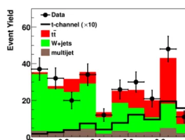
Moreover a decision tree output is by nature discrete, limited by the purities of all leaves in the tree. This means that to decrease the discontinuities one has to increase the tree size and complexity, which may not be desirable or even possible. Then the tendency is to have spikes in the output distribution at specific purity values, as illustrated in Fig. 3, or even two delta functions at±1 if using a binary answer rather than the purity output.

Section 3.2 describes how these shortcomings can for the most part be addressed by averaging.

3.1 Pruning a tree

(8)

Figure 3. Comparison of signal, back-grounds and data for one of the decision tree outputs in an old D0 single top quark search. The discrete output of a decision tree is clearly visible, but data are well re-produced by the model.

on properties of the training sample that may not reflect the expected result, had there been infinite statistics to train on.

A first approach to mitigate this eﬀect, sometimes referred to as pre-pruning, has already been described in Section 2, using stopping conditions. They included requiring a minimum number of events in each node or a minimum amount of separation improvement. The limitation is that requiring too big a minimum leaf size or too much improvement may prevent further splitting that could be very beneficial.

Another approach consists in building a very large tree and then cutting irrelevant branches by turning an internal node and all its descendants into a leaf, removing the corresponding subtree. This is post-pruning, or simply pruning.

Why would one wish to prune a decision tree? It is possible to get a perfect classifier on the train-ing sample: mathematically the misclassification rate can be made as little as one wants on traintrain-ing events. For instance one can build a tree such that each leaf contains only one class of events (down to one event per leaf if necessary). The training error is then zero. But when passing events through the tree that were not seen during training, the misclassification rate will most likely be non-zero, showing signs of overtraining. Pruning helps in avoiding such eﬀects, by eliminating subtrees (branches) that are deemed too specific to the training sample.

There are many diﬀerent pruning algorithms available. Only three of them, among the most commonly used, are presented briefly.

Expected error pruning was introduced by Quinlan [4] in the ID3 algorithm. A full tree is first grown. One then computes the approximate expected error for a node (using the Laplace error estimate E= ne+nc−1

N₊nc , where neis the number of misclassified events out of N events in the node, and ncis the

number of classes, 2 for binary trees), and compares it to the weighted sum of expected errors from its children. If the expected error of the node is less than that of the children, then the node is pruned. This algorithm is fast and does not require a separate sample of events to do the pruning, but it is also known to be too aggressive: it tends to prune large subtrees containing branches with good separation power.

(9)

Cost-complexity pruning is part of the CART algorithm [1]. The idea is to penalise complex trees (with many nodes and/or leaves) and to find a compromise between a good fit to training data (requir-ing a larger tree) and good generalisation properties (usually better achieved with a smaller tree). Consider a fully grown decision tree, Tmax. For any subtree T (with NT nodes) of Tmaxwith a

mis-classification rate R(T ) one can define the cost complexity Rα(T ):

Rα(T )=R(T )+αNT,

whereαis a complexity parameter. When trying to minimise Rα(T ), a smallαwould help picking Tmax(no cost for complexity) while a largeαwould keep only the root node, Tmaxbeing fully pruned.

The optimally pruned tree is somewhere in the middle.

In a first pass, for terminal nodes tPand tF emerging from the split of node t, by construction R(t)≥

R(tP)+R(tF). If these quantities are equal, then one can prune oﬀtPand tF.

Now, for node t and subtree Tt, by construction R(t)>R(Tt) if t is non-terminal. The cost complexity

for node t is:

Rα({t})=Rα(t)=R(t)+α

since Nt=1. If Rα(Tt)<Rα(t), then the branch Tthas smaller cost-complexity than the single node

{t}and should be kept. But for a critical valueα=ρt, obtained by solving Rρt(Tt)=Rρt(t), that is:

ρt=

R(t)−R(Tt)

NT−1

,

pruning the tree and making t a leaf becomes preferable. The node with the smallestρtis the weakest

link and gets pruned. The algorithm is applied recursively on the pruned tree until it is completely pruned, leaving only the root node.

This generates a sequence of decreasing cost-complexity subtrees. For each of them (from Tmax to

the root node), one then computes their misclassification rate on the validation sample. It will first decrease, and then go through a minimum before increasing again. The optimally pruned tree is the one corresponding to the minimum.

It should be noted that the best pruned tree may not be optimal when part of a forest of trees, such as those introduced in the next Sections.

3.2 Averaging several trees

Pruning was shown to be helpful in maximising the generalisation potential of a single decision tree. It nevertheless doesn’t address other shortcomings of trees like the discrete output or the sensitivity of the tree structure to the training sample composition. A way out is to proceed with averaging several trees, with the added potential bonus that the discriminating power may increase, as briefly described in the 2008 proceedings of this school [ 5].

Such a principle was introduced from the beginning with the so-called V-fold cross-validation [ 1], a useful technique for small samples. After dividing a training sampleLinto V subsets of equal size, L = v=1..VLv, one can train a tree Tvon the L − Lv sample and test it onLv. This produces V

decision trees, whose outputs are combined into a final discriminant: 1

V

v=1..V

Tv.

(10)

4 Boosting

As will be shown in this section, the boosting algorithm has turned into a very successful way of improving the performance of any type of classifier, not only decision trees. After a short history of boosting in Section 4.1, the generic algorithm is presented in Section 4.2 and a specific implementation (AdaBoost) is described in Section 4.3. Boosting is illustrated with a few examples in Section 4.4. Finally other examples of boosting implementations are given in Section 4.5.

4.1 A brief history of boosting

Boosting has appeared quite recently. The first provable algorithm of boosting was proposed by Schapire in 1990 [6]. It worked in the following way:

• train a classifier T1on a sample of N events.

• train T2on a new sample with N events, half of which were misclassified by T1.

• build T3on events where T1and T2disagree.

The boosted classifier was defined as a majority vote on the outputs of T1, T2and T3.

In 1995 Freund followed up on this idea [ 7], introducing boosting by majority. It consisted in combining many learners with a fixed error rate. This was an impractical prerequisite for a viable au-tomated algorithm, but was a stepping stone to the proposal by Freund&Schapire of the first functional boosting algorithm, called AdaBoost [8].

Boosting, and in particular boosted decision trees, have become increasingly popular in high en-ergy physics. The MiniBooNe experiment first compared the performance of diﬀerent boosting algo-rithms and artificial neural networks for particle identification [ 9]. The D0 experiment was the first to use boosted decision trees for a search, which lead to the first evidence (and then observation) of single top quark production [10].

4.2 Boosting algorithm

Boosting is a general technique which is not limited to decision trees, although it is often used with them. It can apply to any classifier, e.g., neural networks. It is hard to make a very good discriminant, but is it relatively easy to make simple ones which are certainly more error-prone but are still perform-ing at least marginally better than random guessperform-ing. Such discriminants are called weak classifiers [ 5]. The goal of boosting is to combine such weak classifiers into a new, more stable one, with a smaller error rate and better performance.

Consider a training sampleTkcontaining Nkevents. The ithevent is associated with a weightwki,

a vector of discriminating variablesxiand a class labelyi = +1 for signal,−1 for background. The

pseudocode for a generic boosting algorithm is:

InitialiseT1

forkin 1..Ntree

train classifierTkonTk

assign weightαktoTk

modifyTkintoTk+1

The boosted output is some function F(T1, ..,TNtree), typically a weighted average:

F(i)=

Ntree

k=1

αkTk(xi).

(11)

4.3 AdaBoost

One particularly successful implementation of the boosting algorithm is AdaBoost, introduced by Freund&Schapire [8]. AdaBoost stands for adaptive boosting, referring to the fact that the learning procedure adjusts itself to the training data in order to classify it better. There are many variations on the same theme for the actual implementation, and it is the most common boosting algorithm. It typically leads to better results than without boosting, up to the Bayes limit as will be seen later.

An actual implementation of the AdaBoost algorithm works as follows. After having built tree Tkone should check which events in the training sampleTkare misclassified by Tk, hence defining

the misclassification rate R(Tk). In order to ease the math, let us introduce some notations. Define I: X→I(X) such thatI(X)=1 if X is true, and 0 otherwise. One can now define a function that tells whether an event is misclassified by Tk. In the decision tree output convention of returning only {±1}

it gives:

isMisclassifiedk(i)=I

_y

i×Tk(i)≤0

_,

while in the purity output convention (with a critical purity of 0.5) it leads to:

isMisclassifiedk(i)=Iyi×(Tk(i)−0.5)≤0.

The misclassification rate is now:

R(Tk)=εk=

Nk

i=1w

k

i ×isMisclassifiedk(i)

Nk

i=1w

k i

.

This misclassification rate can be used to derive a weight associated to tree Tk:

αk=β×ln

1−εk

εk

,

whereβis a free boosting parameter to adjust the strength of boosting (it was set to 1 in the original algorithm).

The core of the AdaBoost algorithm resides in the following step: each event inTkhas its weight

changed in order to create a new sampleTk+1such that:

wk

i →w

k+1

i =w

k

i ×e

αk·isMisclassifiedk(i).

This means that properly classified events are unchanged fromTk toTk₊1, while misclassified

events see their weight increased by a factor eαk_{. The next tree T}

k₊1is then trained on theTk₊1sample.

This next tree will therefore see a diﬀerent sample composition with more weight on misclassified events, and will therefore try harder to classify properly diﬃcult events that tree Tkfailed to identify

correctly. The final AdaBoost result for event i is:

T (i)=_N1 tree

k₌1 αk

Ntree

k₌1

αkTk(i).

As an example, assume for simplicity the caseβ=1. A not-so-good classifier, with a misclassifi-cation rateε=40% would have a correspondingα=ln1₀−_.0₄.4 =0.4. All misclassified events would therefore get their weight multiplied by e0.4₌₁_._{5, and the next tree will have to work a bit harder on}

(12)

tree! This shows that being failed by a good classifier brings a big penalty: it must be a diﬃcult case, so the next tree will have to pay much more attention to this event and try to get it right.

It can be shown [11] that the misclassification rateεof the boosted result on the training sample is bounded from above:

ε≤

Ntree

k=1

2εk(1−εk).

If each tree hasεk 0.5, that is to say, if it does better than random guessing, then the conclusion

is quite remarkable: the error rate falls to zero for a suﬃciently large Ntree! A corollary is that the

training data is overfitted.

Overtraining is usually regarded has a negative feature. Does this mean that boosted decision trees are doomed because they are too powerful on the training sample? Not really. What matters most is not the error rate on the training sample, but rather the error rate on a testing sample. This may well decrease at first, reach a minimum and increase again as the number of trees increases. In such a case one should stop boosting when this minimum is reached. It has been observed that quite often boosted decision trees do not go through such a minimum, but rather tend towards a plateau in testing error. One could then decide to stop boosting after having reached this plateau.

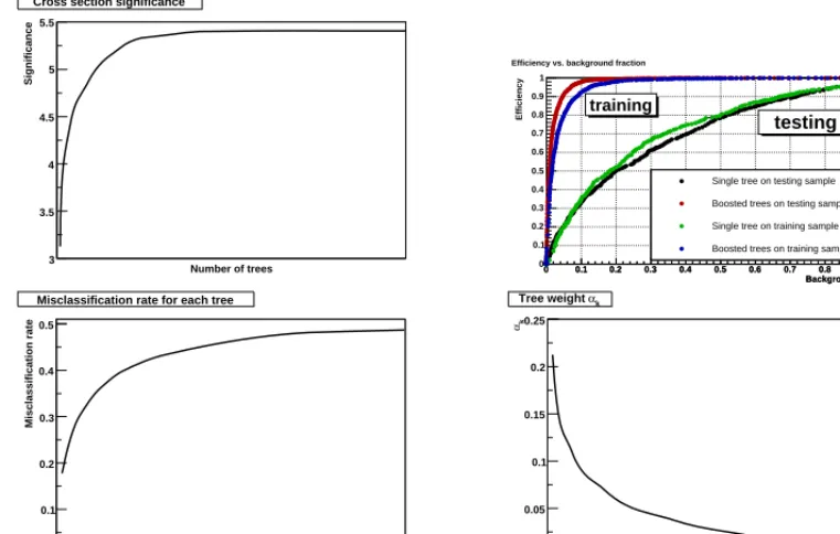
In a typical high energy physics problem, the error rate may not even be what one wants to op-timise. A good figure of merit on the testing sample would rather be the significance. Figure 4 (top left) illustrates this behaviour, showing how the significance saturates with an increasing number of boosting cycles. One could argue one should stop before the end and save resources, but at least the performance does not deteriorate with increasing boosting.

Another typical curve one tries to optimise is the signal efficiency vs. the background efficiency. Figure 4 (top right) clearly exemplifies the interesting property of boosted decision trees. The per-formance is clearly better on the training sample than on the testing sample (the training curves are getting very close to the upper left corner of perfect separation), with a single tree or with boosting, a clear sign of overtraining. But the boosted tree is still performing better than the single tree on the testing sample, proof that it does not suffer from this overtraining.

People have been wondering why boosting leads to such features, with typically no loss of gen-eralisation performance due to overtraining. No clear explanation has emerged yet, but some ideas have come up. It may have to do with the fact that during the boosting sequence, the first tree is the best while the others are successive minor corrections, which are given smaller weights. This is shown at the bottom of Fig. 4, where the misclassification rate of each new tree separately is actually increasing, while the corresponding tree weight is decreasing. This is no surprise: during boosting the successive trees are specialising on specific event categories, and can therefore not perform as well on other events. So the trees that lead to a perfect fit of the training data are contributing very little to the final boosted decision tree output on the testing sample. When boosting decision trees, the last tree is not an evolution of the first one that performs better, quite the contrary. The first tree is typically the best, while others bring dedicated help for misclassified events. The power of boosting does not rely in the last tree in the sequence, but rather in combining a suite of trees that focus on diﬀerent events.

Finally a probabilistic interpretation of AdaBoost was proposed [ 12] which gives some insight into the performance of boosted decision trees. It can be shown that for a boosted output T flexible enough:

eT (i)= p(S|i)

p(B|i) =BD(i),

(13)

Number of trees

Significance

3 3.5 4 4.5 5 5.5

Cross section significance

Background Fraction 0 0.1 0.2 0.3 0.4 0.5 0.6 0.7 0.8 0.9 1 Background Fraction 0 0.1 0.2 0.3 0.4 0.5 0.6 0.7 0.8 0.9 1

Efficiency

0 0.1 0.2 0.3 0.4 0.5 0.6 0.7 0.8 0.9 1

Efficiency vs. background fraction

Single tree on testing sample

Boosted trees on testing sample

Single tree on training sample

Boosted trees on training sample

testing training

Number of trees

Misclassification rate

0 0.1 0.2 0.3 0.4 0.5

Misclassification rate for each tree

Number of trees

k

α

0 0.05 0.1 0.15 0.2 0.25

k α

Tree weight

Figure 4.Behaviour of boosting. Top left: Significance as a function of the number of boosted trees.

Top right: Signal eﬃciency vs. background eﬃciency for single and boosted decision trees, on the training and testing samples. Bottom left: Misclassification rate of each tree as a function of the number of boosted trees. Bottom right: Weight of each tree as a function of the number of boosted trees.

4.4 Boosting practical examples

The examples of this section were produced using the TMVA package [ 14].

4.4.1 A simple 2D example

This example starts from code provided by G. Cowan [ 15]. Consider a system described by two variables, x andy, as shown in Fig. 5.

(14)

Figure 5.x :ycorrelation of input variables used to illustrate how decision trees work. Signal is in blue, background in red.

BDT response

-0.8 -0.6 -0.4 -0.2 0 0.2 0.4 0.6 0.8

Normalized

0 1 2 3 4 5 6

7 Signal

Background

BDT response

-0.8 -0.6 -0.4 -0.2 0 0.2 0.4 0.6 0.8

Normalized

0 1 2 3 4 5 6 7

U/O-flow (S,B): (0.0, 0.0)/ (0.0, 0.0)

TMVA response for classifier: BDT

Signal efficiency

0 0.1 0.2 0.3 0.4 0.5 0.6 0.7 0.8 0.9 1

Background rejection

0.2 0.3 0.4 0.5 0.6 0.7 0.8 0.9 1

0 0.1 0.2 0.3 0.4 0.5 0.6 0.7 0.8 0.9 1

0.2 0.3 0.4 0.5 0.6 0.7 0.8 0.9 1

MVA Method: BDT Fisher DT

Background rejection versus Signal efficiency

Figure 6. Top left: First decision tree built on x andy. Top right: Criteria applied in this first tree,

(15)

4.4.2 The XOR problem

Another way of showing how a decision tree can handle complicated inputs is the XOR problem, a small version of the checkerboard, illustrated in Fig. 7. With enough statistics (left column), even a single tree is already able to find more or less the optimal separation, so boosting cannot actually do much better. On the other hand this type of correlations is a killer for a Fisher discriminant, which fairs as bad as random guessing.

One can repeat the exercise, this time with limited statistics (right column in Fig. 7). Now a single tree is not doing such a good job anymore and the Fisher discriminant is completely unreliable. Boosted decision trees, on the other hand, are doing almost as well as with full statistics, separating almost perfectly signal and background. This illustrates very clearly how the combination of weak classifiers (see for instance the lousy performance of the first tree) can generate a high performance discriminant with a boosting algorithm.

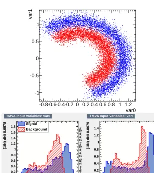
4.4.3 Circular correlation

This example is derived from a dataset generated with thecreate_circmacro from

$ROOTSYS/tmva/test/createData.C. The 1D and 2D representations of the two variables used

are shown in Fig. 8.

Several generic properties can be tested with this dataset: the impact of a longer boosting sequence (adding more and more trees), the meaningfulness of overtraining, the sensitivity to the splitting cri-terion and the diﬀerence between boosting many small trees or few big trees.

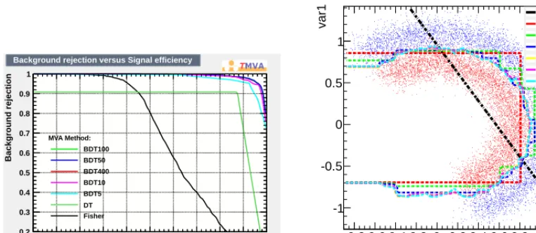
Figure 9 compares the performance of a Fisher discriminant (for reference), a single decision tree and boosted decision trees with an increasing number of trees (from 5 to 400). All other TMVA parameters are kept to their default value. One can see how a Fisher discriminant is not appropriate for non-linear correlation problems. The performance of the single tree is not so good, as expected since the default TMVA parameters make it very small, with a depth of 3 (it should be noted that a single bigger tree could solve this problem easily). Increasing the number of trees improves the performance until it saturates in the high background rejection and high signal eﬃciency corner. It should be noted that adding more trees doesn’t seem to degrade the performance, the curve stays in the optimal corner. Looking at the contour plot one can however see that it wiggles a little for larger boosted decision trees, as they tend to pick up features of the training sample. This is overtraining.

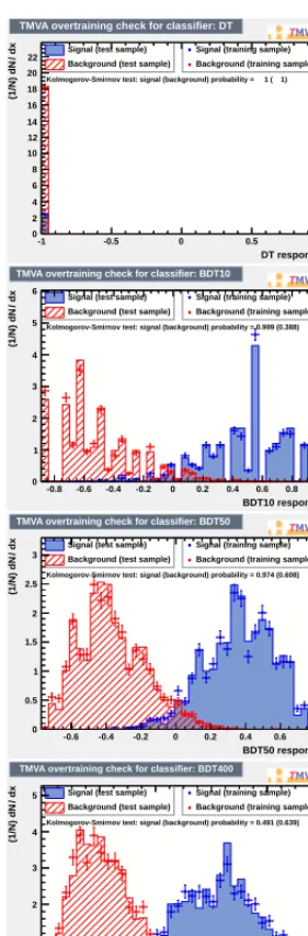
Another sign of overtraining also appears in Fig. 10, showing the output of the various boosted decision trees for signal and background, both on the training and testing samples: larger boosted decision trees tend to show discrepancies between the two samples, as they adjust to peculiarities of the training sample that are not found in an independent testing sample. One can also see how the output acquires a “better” shape with more trees, really becoming quasi-continuous, which would allow to cut at a precise eﬃciency or rejection.

(16)

x 0 0.2 0.4 0.6 0.8 1

y 0 0.2 0.4 0.6 0.8 1 y:x x 0 0.2 0.4 0.6 0.8 1

y 0 0.2 0.4 0.6 0.8 1 y:x BDT response

-0.6 -0.4 -0.2 0 0.2 0.4

Normalized 0 5 10 15 20 25 30 _Signal Background BDT response

-0.6 -0.4 -0.2 0 0.2 0.4

Normalized 0 5 10 15 20 25 30

U/O-flow (S,B): (0.0, 0.0)/ (0.0, 0.0)

TMVA response for classifier: BDT

0 0.1 0.2 0.3 0.4 0.5 0.6 0.7 0.8 0.9 1

Background rejection 0.2 0.3 0.4 0.5 0.6 0.7 0.8 0.9 1 Signal efficiency

0 0.1 0.2 0.3 0.4 0.5 0.6 0.7 0.8 0.9 1

Background rejection 0.2 0.3 0.4 0.5 0.6 0.7 0.8 0.9 1 MVA Method: BDT DT Fisher

0 0.1 0.2 0.3 0.4 0.5 0.6 0.7 0.8 0.9 1

Background rejection 0.2 0.3 0.4 0.5 0.6 0.7 0.8 0.9 1 Signal efficiency

0 0.1 0.2 0.3 0.4 0.5 0.6 0.7 0.8 0.9 1

Background rejection 0.2 0.3 0.4 0.5 0.6 0.7 0.8 0.9 1 MVA Method: BDT Fisher DT

Figure 7. The XOR problem. Signal is in blue, background in red. The left column uses suﬃcient statistics,

(17)

var0 -0.8-0.6-0.4-0.2 0 0.2 0.4 0.6 0.8 1 1.2

var1

-1 -0.5 0 0.5 1

var0

-0.8-0.6-0.4-0.2 0 0.2 0.4 0.6 0.8 1 1.2 1.4

0.0578

/

(1/N) dN

0 0.2 0.4 0.6 0.8 1 1.2 1.4 1.6

1.8 Signal

Background

U/O-flow (S,B): (0.0, 0.0)% / (0.0, 0.0)%

TMVA Input Variables: var0

var1

-1 -0.5 0 0.5 1

0.0679

/

(1/N) dN

0 0.2 0.4 0.6 0.8 1 1.2 1.4

U/O-flow (S,B): (0.0, 0.0)% / (0.0, 0.0)%

TMVA Input Variables: var1

Figure 8. Dataset for the circular correlation example. Top: 2D representation. Bottom: 1D projections.

This example can also be used to illustrate the performance of each tree in a boosting sequence. Figure 12 shows the rapid decrease of the weightαk of each tree, while at the same time the

corre-sponding misclassification rateεkof each individual tree increases rapidly towards just below 50%,

that is, random guessing. It confirms that the best trees are the first ones, while the others are only minor corrections.

(18)

0 0.1 0.2 0.3 0.4 0.5 0.6 0.7 0.8 0.9 1

0.2 0.3 0.4 0.5 0.6 0.7 0.8 0.9 1

MVA Method: BDT100 BDT50 BDT400 BDT10 BDT5 DT Fisher

var0 -0.8-0.6-0.4-0.2 0 0.2 0.4 0.6 0.8 1 1.2

var1

-1 -0.5 0 0.5 1

Fisher DT BDT5 BDT10 BDT50 BDT100 BDT400

Figure 9. Circular correlation example. Left: Background rejection vs. signal eﬃciency curves for a Fisher

discriminant (black), a single decision tree (dark green) and boosted decision trees with an increasing number of trees (5 to 400). Right: Decision contour corresponding to the previous discriminants.

as a function of boosted decision tree output, which confirms that they all reach similar performance while the tree optimised with significance actually performs slightly worse than the others.

A final illustration concerns the impact of the size of each tree in terms of number of leaves and size of each leaf, and their relation to the number of trees. In order to test this, the samecreate_circ

macro was used, but to produce a much larger dataset such that statistics do not interfere with the test. All combinations of boosted decision trees with 20 or 400 trees, a minimum leaf size of 10 or 500 events and a maximum depth of 3 or 20 were tested, and results are shown on Fig. 14 as the decision contour and in terms of background rejection vs. signal eﬃciency curves. One can see an overall very comparable performance.

As is often the case for boosted decision trees, such optimisation on the number and size of trees, size of leaves or splitting criterion depends on the use case. To first approximation it is fair to say that almost any default will do, and optimising these aspects may not be worth the time required to test all configurations.

4.5 Other boosting algorithms

AdaBoost is but one of many boosting algorithms. It is also referred to as discrete AdaBoost to distinguish it from other AdaBoost flavours. The Real AdaBoost algorithm [ 12] defines each decision tree output as:

Tk(i)=0.5×ln

pk(i)

1−pk(i)

,

where pk(i) is the purity of the leaf on which event i falls. Events are reweighted as:

wk

i →w

k+1

i =w

k

i ×e−

(19)

DT response

-1 -0.5 0 0.5 1

dx / (1/N) dN 0 2 4 6 8 10 12 14 16 18 20

22 Signal (test sample) Background (test sample)

Signal (training sample) Background (training sample)

Kolmogorov-Smirnov test: signal (background) probability = 1 ( 1)

U/O-flow (S,B): (0.0, 0.0)% / (0.0, 0.0)%

TMVA overtraining check for classifier: DT

BDT5 response

-1 -0.5 0 0.5 1

dx / (1/N) dN 0 1 2 3 4 5 6 7 8

Kolmogorov-Smirnov test: signal (background) probability = 0.837 ( 1)

U/O-flow (S,B): (0.0, 0.0)% / (0.0, 0.0)%

TMVA overtraining check for classifier: BDT5

BDT10 response

-0.8 -0.6 -0.4 -0.2 0 0.2 0.4 0.6 0.8 1

dx / (1/N) dN 0 1 2 3 4 5 6

Signal (test sample) Background (test sample)

Kolmogorov-Smirnov test: signal (background) probability = 0.999 (0.388)

U/O-flow (S,B): (0.0, 0.0)% / (0.0, 0.0)%

BDT50 response

-0.6 -0.4 -0.2 0 0.2 0.4 0.6 0.8

dx / (1/N) dN 0 0.5 1 1.5 2 2.5 3

Signal (test sample) Background (test sample)

U/O-flow (S,B): (0.0, 0.0)% / (0.0, 0.0)%

BDT100 response

-0.6 -0.4 -0.2 0 0.2 0.4 0.6

dx / (1/N) dN 0 0.5 1 1.5 2 2.5 3 3.5

4 _{Signal (test sample)} Background (test sample)

Kolmogorov-Smirnov test: signal (background) probability = 0.952 ( 0.95)

U/O-flow (S,B): (0.0, 0.0)% / (0.0, 0.0)%

BDT400 response

-0.4 -0.2 0 0.2 0.4

dx / (1/N) dN 0 1 2 3 4

U/O-flow (S,B): (0.0, 0.0)% / (0.0, 0.0)%

Figure 10. Circular correlation example. Comparison of the output on training (markers) and testing (histograms)

samples for boosted decision trees with 1, 5, 10, 50, 100 and 400 trees (from top left to bottom right).

and the boosted result is T (i)= Ntree

k=1 Tk(i). Gentle AdaBoost and LogitBoost (with a logistic

func-tion) [12] are other variations.

ε-Boost, also called shrinkage [16], consists in reweighting misclassified events by a fixed factor e2ε_{rather than the tree-dependent}_α

(20)

Cut value applied on DT output

-1 -0.5 0 0.5 1

Efficiency (Purity) 0.5 0.6 0.7 0.8 0.9 1 1.1 Signal efficiency Background efficiency Signal purity Signal efficiency*purity S+B S/

For 1000 signal and 1000 background is S+B events the maximum S/ 28.1146 when cutting at -0.9997 Cut efficiencies and optimal cut value

Significance 0 5 10 15 20 25 30

Cut value applied on BDT5 output

-1 -0.5 0 0.5 1

Efficiency (Purity) 0.2 0.4 0.6 0.8 1 Signal efficiency Background efficiency Signal purity Signal efficiency*purity S+B S/

For 1000 signal and 1000 background is S+B events the maximum S/ 29.6995 when cutting at 0.0431 Cut efficiencies and optimal cut value

Significance 0 5 10 15 20 25 30

-0.8 -0.6 -0.4 -0.2 0 0.2 0.4 0.6 0.8 1

Efficiency (Purity) 0 0.2 0.4 0.6 0.8 1 Signal efficiency Background efficiency Signal purity Signal efficiency*purity S+B S/

Significance 0 5 10 15 20 25 30

-0.6 -0.4 -0.2 0 0.2 0.4 0.6 0.8

Significance 0 5 10 15 20 25 30

-0.6 -0.4 -0.2 0 0.2 0.4 0.6

For 1000 signal and 1000 background is S+B events the maximum S/ 30.3106 when cutting at 0.0024 Cut efficiencies and optimal cut value

Significance 0 5 10 15 20 25 30

-0.4 -0.2 0 0.2 0.4

Significance 0 5 10 15 20 25 30

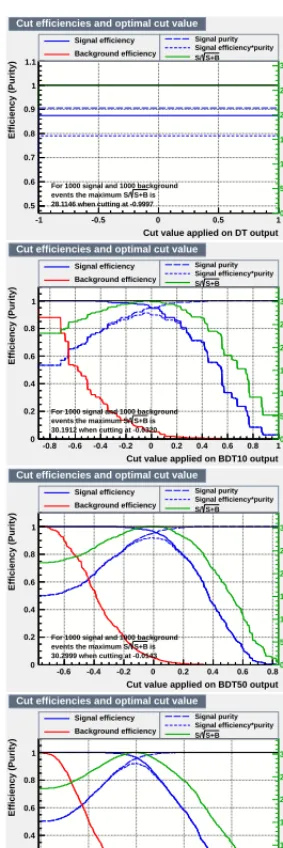
Figure 11. Circular correlation example. Signal eﬃciency, background eﬃciency, signal purity and significance

s/√s+b for boosted decision trees with 1, 5, 10, 50, 100 and 400 trees (from top left to bottom right).

a logistic function e−yi Tk (i)

1+e−yi Tk (i).ε-HingeBoost [9] is only dealing with misclassified events:

wk

i →w

k+1

i =I(yi×Tk(i)≤0).

(21)

con-Figure 12. Circular correlation example, with a 400-tree boosted decision tree. Left: Boost weight of each tree. Right: Error fraction of each tree.

tribution to the total result, modelling this limit with the diﬀerential equations that govern Brownian motion.

5 Other averaging techniques

As mentioned in Section 3.2 the key to improving a single decision tree performance and stability is averaging. Other techniques than boosting exist, some of which are briefly described below. As with boosting, the name of the game is to introduce statistical perturbations to randomise the training sample, hence increasing the predictive power of the ensemble of trees [ 5].

Bagging (Bootstrap AGGregatING) was proposed by Breiman [ 18]. It consists in training trees on diﬀerent bootstrap samples drawn randomly with replacement from the training sample. Events that are not picked for the bootstrap sample form an “out of bag” validation sample. The bagged output is the simple average of all such trees.

Random forests is bagging with an extra level of randomisation [ 19]. Before splitting a node, only a random subset of input variables is considered. The fraction can vary for each split for yet another level of randomisation.

Trimming is not exactly an averaging technique per se but can be used in conjunction with another technique, in particular boosting, to speed up the training process. After some boosting cycles, it is possible that very few events with very high weight are making up most of the total training sample weight. One may then decide to ignore events with very small weights, hence introducing again some minor statistical perturbations and speeding up the training.ε-HingeBoost is such an algorithm.

(22)

0.55 0.6 0.65 0.7 0.75 0.8 0.85 0.9 0.95

Background rejection 0.7 0.75 0.8 0.85 0.9 0.95 1 MVA Method: CrossEntropy GiniWithLaplace Gini MisclassificationError SDivSqrtSPlusB

Cut value applied on CrossEntropy output

-0.4 -0.2 0 0.2 0.4 0.6

Significance 0 5 10 15 20 25 30

Cut value applied on Gini output

-0.4 -0.2 0 0.2 0.4

Significance 0 5 10 15 20 25 30

Cut value applied on GiniWithLaplace output

-0.4 -0.3 -0.2 -0.1 0 0.1 0.2 0.3 0.4 0.5

Significance 0 5 10 15 20 25 30

Cut value applied on MisclassificationError output

-0.4 -0.3 -0.2 -0.1 0 0.1 0.2 0.3 0.4

Significance 0 5 10 15 20 25 30

Cut value applied on SDivSqrtSPlusB output

-0.8 -0.6 -0.4 -0.2 0 0.2 0.4 0.6 0.8

Significance 0 5 10 15 20 25 30

Figure 13. Circular correlation example: impact of the choice of splitting function. Top left: Background rejection vs.

signal efficiency. From top middle to bottom left: Signal efficiency, background efficiency, signal purity and significance

s/√s+b for cross entropy, Gini index, Gini index with Laplace correction, misclassification error and s/√s+b.

6 Conclusion

(23)

var0 -0.8-0.6-0.4-0.2 0 0.2 0.4 0.6 0.8 1 1.2 1.4

var1

-1 -0.5 0 0.5 1

BDT default BDT400_minevt500_maxdepth3 BDT400_minevt500_maxdepth20 BDT400_minevt10_maxdepth3 BDT400_minevt10_maxdepth20 BDT20_minevt500_maxdepth3 BDT20_minevt500_maxdepth20 BDT20_minevt10_maxdepth3 BDT20_minevt10_maxdepth20

0 0.1 0.2 0.3 0.4 0.5 0.6 0.7 0.8 0.9 1

0.6 0.65 0.7 0.75 0.8 0.85 0.9 0.95 1

MVA Method: BDT

BDT400_minevt10_maxdepth3 BDT400_minevt500_maxdepth3 BDT20_minevt500_maxdepth3 BDT20_minevt10_maxdepth3 BDT400_minevt500_maxdepth20 BDT20_minevt500_maxdepth20 BDT20_minevt10_maxdepth20 BDT400_minevt10_maxdepth20

Figure 14. Circular correlation example with larger dataset and boosted decision trees with 20 or 400 trees,

a minimum leaf size of 10 or 500 events and a maximum depth of 3 or 20. Left: Decision contour for each combination. Right: Background rejection vs. signal eﬃciency for each combination.

results (not black boxes) with possible interpretation by a physicist, can deal easily with all sorts of variables and with many of them, with in the end relatively few parameters.

Decision trees are, however, not perfect and suﬀer from the piecewise nature of their output and a high sensitivity to the content of the training sample. These shortcoming are for a large part addressed by averaging the results of several trees, each built after introducing some statistical perturbation in the training sample. Among the most popular such techniques, boosting (and its AdaBoost incarnation) was described in detail, providing ideas as to why it seems to be performing so well and being very resilient against overtraining. Other averaging techniques were briefly described.

Boosted decision trees have now become quite fashionable in high energy physics. Following the steps of MiniBooNe for particle identification and D0 for the first evidence and observation of single top quark production, other experiments and analyses are now using them, in particular at the LHC. This warrants a word a caution. Despite recent successes in several high profile results, boosted decision trees cannot be thought of as the best multivariate technique around. Most multivariate techniques will in principle tend towards the Bayes limit, the maximum achievable separation, given enough statistics, time and information. But in real life resources and knowledge are limited and it is impossible to know a priori which method will work best on a particular problem. The only way is to test them. Figure 15 illustrates this situation for the single top quark production evidence at D0 [ 10]. In the end boosted decision trees performed only marginally better than Bayesian neural networks and the matrix elements technique, but all three analyses were very comparable, as shown by their power curves. The boosted decision tree analysis profited, however, of the fast turnaround of decision tree training in order to perform many valuable cross checks.

(24)

Figure 15. Comparison of several analysis techniques used in the D0 search for single top quark produc-tion [10]. Left: Signal vs. background eﬃciency curves for random guessing, a cut-based analysis, artificial neural networks, decision trees, Bayesian neural networks, the matrix elements technique and boosted decision trees. Right: Power curves (p-value of the signal+background hypothesis vs. p-value of the background-only hypothesis) for the boosted decision trees, Bayesian neural networks and matrix elements.

7 Software

Many implementations of decision trees exist on the market. Historical algorithms like CART [ 1], ID3 [20] and its evolution C4.5 [21] are available in many diﬀerent computing languages. The orig-inal MiniBoone [9] code is available at http://www-mhp.physics.lsa.umich.edu/∼roe/, so is the Stat-PatternRecognition [2] code at http://sourceforge.net/projects/statpatrec, and LHC experiments have various implementations in their software.

I would recommend a diﬀerent approach, which is to use an integrated solution able to handle decision trees but also other techniques and flavours, allowing to run several of them to find the best suited to a given problem. Weka is a data mining software written in Java, open source, with a very good published manual. It was not written for HEP but is very complete. Details can be found at http://www.cs.waikato.ac.nz/ml/weka/.

Another recent development, now popular in HEP, is TMVA [ 14]. It is integrated in recent ROOT releases, which makes it convenient to use, and comes with a complete manual. It is also available online at http://tmva.sourceforge.net.

8 Acknowledgements

I would like to thank the organisers for their continuing trust in my lectures on decision trees. The school program, lectures, attendance and location were once again very enjoyable.

References

[1] L. Breiman, J.H. Friedman, R.A. Olshen and C.J. Stone, Classification and Regression Trees, Wadsworth, Stamford, 1984

(25)

[3] C. Gini, “Variabilità e Mutabilità” (1912), reprinted in Memorie di Metodologica Statistica, edited by E. Pizetti and T. Salvemini, Rome: Libreria Eredi Virgilio Veschi, 1955.

[4] J.R. Quinlan, “Simplifying decision trees”, International Journal of Man-Machine Studies, 27(3):221–234, 1987.

[5] H. Prosper, Multivariate discriminants, “Ensemble learning”, EPJ Web of Conferences 4 02001, 2010, SOS’08 - School of Statistics.

[6] R.E. Schapire, “The strength of weak learnability”, Machine Learning, 5(2):197–227, 1990. [7] Y. Freund, “Boosting a weak learning algorithm by majority”, Information and Computation.

121(2):256–285, 1995.

[8] Y. Freund and R.E. Schapire, “Experiments with a New Boosting Algorithm” in Machine Learn-ing: Proceedings of the Thirteenth International Conference, edited by L. Saitta (Morgan Kauf-mann, San Francisco) p. 148, 1996.

[9] B.P. Roe, H.-J. Yang, J. Zhu, Y. Liu, I. Stancu, and G. McGregor, Nucl. Instrum. Methods Phys. Res., Sect.A 543, 577, 2005; H.-J. Yang, B.P. Roe, and J. Zhu, Nucl. Instrum. Methods Phys. Res., Sect. A 555, 370, 2005.

[10] V. M. Abazov et al. [D0 Collaboration], “Evidence for production of single top quarks and first direct measurement of|Vtb|”, Phys. Rev. Lett. 98, 181802, 2007; V. M. Abazov et al., “Evidence

for production of single top quarks”, Phys. Rev. D78, 012005, 2008; V. M. Abazov et al., “Ob-servation of single top quark production”, Phys. Rev. Lett. 103, 092001, 2009.

[11] Y. Freund and R.E. Schapire, “A decision-theoretic generalization of on-line learning and an application to boosting”, Journal of Computer and System Sciences, 55(1):119–139, 1997. [12] J.H. Friedman, T. Hastie and R. Tibshirani, “Additive logistic regression: a statistical view of

boosting”, The Annals of Statistics, 28(2), 377–386, 2000.

[13] H. Prosper, Multivariate discriminants, “Optimal classification”, EPJ Web of Conferences 4 02001, 2010, SOS’08 - School of Statistics.

[14] A. Höcker et al., “TMVA: Toolkit for multivariate data analysis”, PoS ACAT, 040, CERN-OPEN-2007-007, arXiv:physics/0703039, 2007.

[15] G. Cowan, “Multivariate statistical methods and data mining in particle physics”, CERN Aca-demic Training Lectures, June 2008. http://indico.cern.ch/event/24827

[16] J.H. Friedman, “Greedy function approximation: a gradient boosting machine”, The Annals of Statistics, 29 (5), 1189–1232, 2001.

[17] Y. Freund, “An adaptive version of the boost by majority algorithm”, Machine Learning, 43 (3), 293–318, 2001.

[18] L. Breiman, “Bagging Predictors”, Machine Learning, 24 (2), 123–140, 1996. [19] L. Breiman, “Random forests”, Machine Learning, 45 (1), 5–32, 2001.

[20] J.R. Quinlan, “Induction of decision trees”, Machine Learning, 1(1):81–106, 1986.