DOI: 10.1051/epjconf/20135301006 C
Owned by the authors, published by EDP Sciences, 2013
Mass composition working group report
E. Barcikowski
1, J. Bellido
2,a, J. Belz
1, Y. Egorov
3, S. Knurenko
3, V. de Souza
4,
Y. Tameda
5, Y. Tsunesada
6, M. Unger
7for the HiRes, Pierre Auger,
Telescope Array and Yakutsk Collaborations
b1Physics Department, University of Utah, USA
2University of Adelaide, Adelaide, S.A. 5005, Australia
3Yu. G. Shafer Institute for Cosmophysical Research and Aeronomy, 31 Lenin Ave.,
677980 Yakutsk, Russia
4Universidade de São Paulo, Instituto de Física de São Carlos, SP, Brazil
5Institute for Cosmic Ray Research, the University of Tokyo, Kashiwa, Chiba 277-8582,
Japan
6Graduate School of Science and Engineering, Tokyo Institute of Technology, Meguro,
Tokyo 152-8550, Japan
7Karlsruhe Institute of Technology, Campus North, Institut für Kernphysik, Karlsruhe,
Germany
Abstract. We present a summary of the measurements of mass sensitive parameters at the highest cosmic
ray energies done by several experiments. TheXmaxdistribution as a function of energy has been measured with fluorescence telescopes by the HiRes, TA and Auger experiments and with Cherenkov light detectors by Yakutsk. The Xmax or the average mass (lnA) has been also inferred using ground detectors, such as muon and water Cherenkov detectors. We discuss the different data analyses elaborated by each collaboration in order to extract the relevant information. Special attention is given to the different approaches used in the analysis of the data measured by fluorescence detectors in order to take into account detector biases. We present a careful analysis of the stability and performance of each analysis. The results of the different experiments will be compared and the discrepancies or agreements will be quantified.
1. INTRODUCTION
In preparation for this meeting, several working groups were formed to establish a common view on the experimental status of measurements at ultra-high energies. Here we report the findings of the mass
composition working group consisting of members of the Auger, HiRes, Telescope Array (TA) and
Yakutsk collaborations. The aim was to understand and quantify potential differences between different experimental results and to try to discuss the measurements in terms of the cosmic ray mass composition. A current issue in the field of ultra high energy cosmic rays is that the measurements [1] of the depth of shower maximum from Auger are shallower and less fluctuating than predictions from air shower simulations for a pure proton composition at energies1019eV. On the other hand, the HiRes and TA
results [3,4] in the same energy regions are consistent with QGSJet-II simulations assuming a constant composition dominated by light elements.
ae-mail:
bFor the full authorlist see Appendix “Collaborations” in this volume.
However, there are important differences in the analysis of the data between Auger, HiRes and TA. In this note we will review the differences between the analyses, compare the different experiment results, and evaluate their compatibility within the experimental statistical and systematic uncertainties.
The main focus of this work is the understanding of the apparent differences between the Auger, HiRes and TAXmaxresults. Nevertheless, we also discuss in this paper other shower observables which
are sensitive to the mass of the primary cosmic rays. The Yakutsk experiment has muon detectors operating and this information is used to inferlnA in a complementary way [5]. In a similar way, the Auger collaboration operates an array of water Cherenkov detectors [6] that are able to measure the muonic and electromagnetic signal at the ground level. This signal is used to inferlnA.
The challenge for determining the cosmic ray mass composition at the highest energy is our limited knowledge of the hadronic interaction properties. The current hadronic interaction models extrapolate interaction properties measured in particle accelerators at energies more than two orders of magnitude smaller. If we knew the hadronic interaction properties at these higher energies, the interpretation of the data in terms of the primary cosmic ray composition would be straightforward. Despite this limitation, we used the hadronic interaction models to convert the different observables measured by each experiment intolnAto allow direct comparison of the measurements.
2. DIFFERENT APPROACHES TO ANALYSEXMAXOBSERVATIONS
The fluorescence detectors (FDs) of the Auger [7], HiRes [8] and TA [9] experiments have a limited field of view (FOV) ranging from about 3◦to 30◦in elevation. This limited FOV introduces a detector bias depending on the shower geometry: For close by showers, the lack of a high elevation FOV prevents the observation of shallow showers and, therefore, deeper showers are favored in the event selection. Moreover, deep near-vertical showers may reach their maximum below the FOV range (or even below ground level) and therefore the ensemble of selected showers is artificially enriched with shallow showers. To address this problem the collaborations follow two different approaches.
2.1 The auger approach
The goal of the Auger Collaboration is to publishXmaxand RMS(Xmax) values with minimal detector
bias, that are close to the moments of the undistorted distribution. This procedure is only limited by systematic uncertainties. The advantage of this proposal is that the published results can be compared directly with model expectations, without the need of any knowledge of the detector and, therefore, also to simulations with hadronic interaction models and or composition hypotheses that were not available at the time of publication.
In order to measure an unbiasedXmaxdistribution, it is necessary to select events based only on their
arriving geometry and energy (i.e. not using any information of theirXmaxvalue). The basic idea is to
select showers with geometries that will allowXmaxto be inside a detector FOV that is “wide enough”
to cover the trueXmaxdistribution. In order to choose the appropriate geometries to be considered in the Xmaxanalysis, it is necessary to have a rough idea of what the range of theXmaxdistribution is. The idea
is to use the data themselves to determine this range for each energy bin.
Given the geometry and energy of an event, the range inXmaxfor which a shower can be detected
with good quality can be predicted with a semi-analytical calculation that takes into account the atmospheric attenuation and the optical efficiency of the detector. The result of such a calculation is anXmax -range, Xminfov to Xmaxfov, for which a shower will be accepted for the data analysis defining the
effective (as opposed to geometrical) FOV of the telescopes.
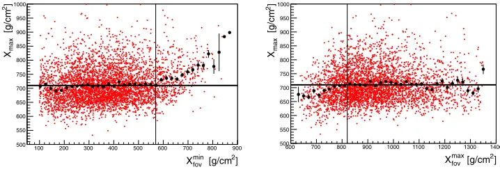
Fig.1 shows the scatter plots of the measuredXmax between 1018.0and 1018.2eV as a function of
the estimated Xmin
fov and Xmaxfov as well as the dependence of the averageXmaxvalues on these variables.
The two plots clearly illustrate the resulting bias that is introduced when Xmin
fov is too deep (panel on the
]
2
[g/cm
fov min
X
100 200 300 400 500 600 700 800 900
]
2
[g/cm
max
X
500 550 600 650 700 750 800 850 900 950 1000
]
2
[g/cm
fov max
X
600 700 800 900 1000 1100 1200 1300 1400
]
2
[g/cm
max
X
500 550 600 650 700 750 800 850 900 950 1000
Figure 1. Scatter plots of the measuredXmaxbetween 1018.0and 1018.2eV as a function of the event-by-event field of view boundaries Xmin
fov and Xmaxfov. The meanXmaxvalues as a function of Xminfov and Xmaxfov are superimposed as large black dots. The horizontal lines denote the asymptoticXmaxvalue far away from the field of view boundary. The range where theXmaxvalues are consistent with this line defines the unbiased region. The vertical lines indicate the limits of fiducial field of view that result in an unbiasedXmaxmeasurement.
Table 1. Number of events above 1018.2eV and 1019.0eV (Fig.6). In this table we have included the number of reconstructed Auger events that survived all the quality cuts (i.e. number of events prior to the application of the field-of-view cuts). The energy distribution of these data is not shown in Fig.6. The total number of events that the HiRes collaboration has used for theXmax analysis above 1018.2eV is 815. However, after the application of the energy normalization (normalized to the TA energy scale) across experiments, 798 HiRes events remained with energies above 1018.2eV (17 events ended up with energies below this). The HiRes collaboration applies a cut on Rp to reduce the detector bias effect. This table shows the number of events before applying this Rp cut.
Auger Auger HiRes HiRes TA Yakutsk
standard cuts without FOV cuts standard cuts no Rp cuts
E>1018.2eV 5138 11343 798 1306 279 412
E>1019.0eV 452 709 123 143 67 22
these graphs for each energy bin in order to determine what ranges of Xmin
fov and Xmaxfov values allow for
an unbiased sampling of theXmax distributions as a function of energy [10,11]. The vertical lines in
Figure1indicates the appropriate limits for Xmin
fov and Xmaxfov . These limits determine the fiducial
field-of-view cuts. These fiducial field-of-field-of-view cuts are optimized independently for the data and for each Monte Carlo (MC) composition. Different MC compositions (i.e. differentXmaxdistributions) have been used
to test this algorithm [10,11] and the reconstructedXmaxvalues were found consistent with the MC
input within statistical uncertainties.
The Auger collaboration applies identical quality cuts to data and Monte Carlo, which is similar to the approach shared by HiRes and TA (in the analysis described below) in which equivalent cuts are applied to data and Monte Carlo throughout. The additional field-of-view cuts – for which there is no direct analog in the HiRes or TA analysis – are optimized independently for the data and for each MC composition, using the same algorithm for this optimization. The motivation behind this choice is to allow optimization of the field-of-view cuts without making any a priori assumptions as to the range of theXmaxdistribution.
Above 1018.2eV, the application of the field-of-view cuts reduce the Auger statistics by half
(Table1). The severity of these field-of-view cuts (for reducing the statistics) puts a constraint on the minimum number of events required for this approach.
2.2 The HiRes and TA approach
detector (we will refer it as Xmeas
max). These twoXmaxvalues can differ significantly depending on
the intrinsic Xmax distribution, or depending on the zenith angle distribution of the events (as shown
in Figs. 8(b) and 8(c)). However, this should not affect the HiRes/TA Xmax composition analysis,
because an accurate detector modeling is used for predicting the Xmeas
max observations for a given
composition.
In order to understand the acceptance and reconstruction biases arising from the inherent field-of-view limitations of a fluorescence detector, both the HiRes and TA collaborations focus on accurate detector modeling through the use of a detailed detector Monte Carlo. Air showers are generated using CORSIKA [12] and several hadronic interaction models including QGSJet01 [13], QGSJet-II [14] and SIBYLL [15, 16]. Shower libraries are created in which the number of particles as a function of slant depth is recorded for a large number of air showers induced by different primary masses.
In the detector simulation, an event is drawn from the library and assigned a random core location, zenith and azimuthal angle. The fluorescence light is propagated from the shower to the detector, with attenuation simulated via the use of an empirically determined atmospheric database. Ray tracing is performed to determine the photoelectron response of individual PMT’s in the fluorescence camera. The trigger algorithms are simulated, and if the trigger conditions are satisfied the Monte Carlo event is written to disk in the identical format as real data, allowing study by the same analysis chain.
A number of control distributions are checked for agreement between data and Monte Carlo in order to assure that all detector effects are accurately described by the simulation. Particular attention is paid to those distributions – e.g. first and last viewed depth of the shower – which touch closely on the detector biasing issue. Finally, to extract information about composition the observedXmax distributions in the
data are compared to the “observed” Xmax distributions for Monte Carlo events which pass identical
event selection criteria.
In summary, in order to estimate an average mass composition, theXmaxmeasured by Auger can
be compared directly with the predictions from air shower simulations (within remaining systematic uncertainties). In the case of HiRes and TA, the measured Xmeas
max should be compared with the
Xmeas
max obtained from a convolution of simulated showers with a model of the detector, atmosphere
and reconstruction.
It is important to note that theXmaxmeasurements by Auger and Yakutsk cannot be compared
directly with the Xmeas
max published by HiRes and TA. In Sec.7 we will transform theseXmaxand
Xmeas
maxtolnAto compare the different experiment results.
3. YAKUTSK MEASUREMENT OF THEXMAXDISTRIBUTIONS
The determination ofXmaxin individual showers is based on the measurement of the Cherenkov light
flux at different core distances Q(r):
1. by the parameter p=lg(Q(200)/Q(500));
2. reconstruction of a shower development curve from the lateral distribution of Cherenkov light [17]; 3. measurement of the Cherenkov light pulse width at a fixed core distance;
4. by recording a Cherenkov track with a differential detector based on camera obscura.
The sensitivity of these techniques is described in [18]. The accuracy of Xmax determination
in individual showers was estimated in a simulation of EAS characteristics measurements at the array involving MC methods and amounted to 30–45 g/cm2, 35–55 g/cm2, 15–25 g/cm2,
35–55 g/cm2 respectively for the first, second, third and fourth methods. The total error of X max
E [eV]
18
10
10
19]
2
[g/cm
650 700 750 800 850
〉 max X 〈 Auger
〉 max X 〈 Yakutsk
〉 meas max X 〈 HiRes
〉 meas max X 〈 TA
Figure 2.Xmaxmeasured by Auger and Yakutsk, together with theXmaxmeasas measured by HiRes and TA. Data points are shifted to a common energy scale (text for details).
E [eV]
18
10 1019
]
2
[g/cm
〉
max
X
〈
550 600 650 700 750 800
850 proton
iron
QGSJet01 QGSJetII SIBYLL2.1 EPOSv1.99
Auger
Yakutsk Auger
Yakutsk
E [eV]
18
10 1019
]
2
) [g/cm
max
RMS(X
0 10 20 30 40 50 60
70 proton
iron
Figure 3. MeasuredXmax(left) and RMS(Xmax) (right) for the Auger and Yakutsk experiments. The lines indicate theXmaxexpectations for proton and iron compositions using different hadronic interaction models. Notice that the highest energy bin for Yakutsk contains only 3 events (Fig.6).
4. COMPARING DIFFERENTXMAXMEASUREMENTS
Figure 2 shows theXmax measured by Auger [19] and Yakutsk [20], together with theXmaxmeas as
measured by HiRes [3] and TA [4]. The observed agreement between the measuredXmaxandXmaxmeas
is not expected.
At this meeting, the energy spectrum working group has compared the shape of the energy spectrum from the Auger, Yakutsk, HiRes and TA experiments and has produced a table with normalization factors [22]. For the plots presented here, we have normalized the energy scales to an energy scale that is half way between the Auger and TA energy scales. The normalization factors that we have used are 1.102 for Auger, 0.55 for Yakutsk, 0.883 for HiRes and 0.908 for TA. Later in Sec.7we will evaluate the compatibility of the different results. We will transformXmaxandXmaxmeastolnAfor meaningful
comparisons.
Figure 3shows the measured Xmax (panel on the left) and RMS(Xmax) (panel on the right) for
the Auger and Yakutsk experiments. Since both experiments publishedXmax values with minimum
E [eV] 18
10 1019
]
2
[g/cm
〉
meas max
X
〈
650 700 750 800 850
proton
iron QGSJet01
QGSJetII
SIBYLL2.1
E [eV]
19
10
]
2
[g/cmX
σ
0 10 20 30 40 50 60
70 QGSJetII
proton
iron
Figure 4. The Xmeas
max (left) and RMS(Xmax) (right) as measured by the HiRes experiment. The lines are the correspondingXmeas
maxandXexpectations for proton and iron compositions. The different line types correspond
to different models.
E [eV] 18
10 1019
]
2
[g/cm
〉
meas max
X
〈
650 700 750 800
850 QGSJet01 QGSJetII SIBYLL2.1
proton
iron
Figure 5. TheXmeas
maxmeasured by the TA experiment. The lines are the correspondingX meas
maxexpectations for proton and iron primaries. The different line types correspond to different models.
for proton and iron compositions. There are different line types corresponding to different high energy hadronic interaction models: QGSJet-01, QGSJet-II, SIBYLL2.1 and EPOSv1.99.
The HiRes collaboration chooses a fluctuation estimator that differs from the one published by Auger and Yakutsk. Whereas the latter use simply the standard deviation (denoted by RMS(Xmax)), HiRes uses
the width of an unbinned likelihood fit with a Gaussian to the distribution truncated at 2×RMS, denoted byX.
Figure4shows theXmeas
maxandXas measured by HiRes. The lines are the correspondingXmeasmax
andXexpectations for proton and iron compositions. The different line types correspond to different
models (QGSJet-01, QGSJet-II, SIBYLL2.1).
Figure 5 shows the corresponding Xmaxmeas observation and expectation for the TA experiment.
Currently the TA experiment does not have enough statistics to quantify the width of the Xmax
distributions at the highest energies.
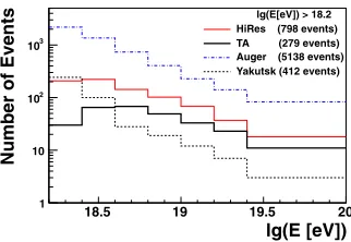
Figure6shows the energy distributions and total number of events that survived the selection cuts at each experiment. For this Figure, the energy scales have been normalized to the TA energy scale. A summary of Figure6is shown in Table1.
TheXmax measurements from Yakutsk (Fig.3), HiRes (Fig.4) and TA (Fig.5) experiments are
consistent with the QGSJet predictions for a constant proton composition at all energies above 1018eV,
whereas theXmaxmeasurements from the Pierre Auger Observatory are significantly shallower than
these predictions above a few EeV (cf. left panel Fig.3).
At the same time, the width of theXmaxdistribution measured by Auger gets narrower above a few
EeV and the Yakutsk measurements of the fluctuations are consistent with the Auger up to about 1019eV.
lg(E [eV])
18.5 19 19.5 20
Number of Events
1 10 2 10 3 10
lg(E[eV]) > 18.2 HiRes (798 events) TA (279 events) Auger (5138 events) Yakutsk (412 events)
Figure 6. Number of events that survived the selection cuts as a function of energy. For this plot the energies have
been normalized to the TA energy scale.
number of events
20 40 60 80 100
]
2
distribution width [g/cm
max X 10 20 30 40 50 60 70 80 p RMS p σ fe RMS fe σ ) 2
p-fe RMS separation (32 g/cm )
2
separation (23 g/cm σ
p-fe
number of events 20 40 60 80 100
]
2
statistical uncertainty [g/cm
0 5 10 15 20 25
number of events
20 40 60 80 100
discrimination performance 0 1 2 3 4 5 6 ideal detector RMS σ 2
resolution = 20 g/cm
max
X RMS σ
Figure 7. Left: Average value of the measured RMS andXas a function of the number of events in the sample.
(middle) Statistical uncertainty of the measured RMS andX. Right: Sensitivity or discrimination power for the
RMS andXapproaches.
about 3 standard deviations (right panel Fig.3). TheXmax distribution widths measured by HiRes at
energies above 2×10¹⁹eV, while consistent with pure proton composition have large statistical errors
and do not definitely exclude a heavier composition (right panel Fig.4).
4.1 A toy MC to evaluate the performance of different fluctuation measures
TheXmaxdistribution is expected to have an asymmetric long tail due to the exponential nature of the
depth of the first interaction. Both, RMS(Xmax) andX , could be under-estimated if they are sampled
with a small number of events. We have used a toy MC simulation to evaluate the performance of both methods for the quantification of the shower-to-shower fluctuations ofXmax.
We have generated random samples of “N” events withXmaxdistributed following the expectation
for 1019eV proton and iron showers using the QGSJet-II model. Fig.7(left panel) shows the measured
RMS andXas a function of the number of events “N”. As can be seen, both approaches show a bias
in the measuredXmaxdistribution width when the number of events in the sample is small. For samples
with at least 30 events, this bias is negligible. Even for smaller statistics, the magnitude of the bias from under-sampling is negligible compared with the statistical uncertainty. The statistical uncertainties for the measured RMS andXare shown in the middle panel of Fig.7.
When using the RMS to quantify theXmax distribution width, the separation between proton and
iron compositions is larger. On the other hand, the associated statistical uncertainties are smaller when usingX. In order to evaluate the performance of using the RMS or theXto quantify the width of the
Xmaxdistribution, we have computed a performance indicator defined as:
sensitivity= width(p/Fe) 2
p+2Fe
lg(E[eV])
18 18.5 19 19.5 20
]
-2
[g cm
〉
Xmax
〈
550 600 650 700 750 800 850
° >38 θ
° <38 θ
(a) Auger Xmax (b) HiRes Xmeasmax (c) HiRes Xmeasmax
Figure 8. TheXmaxandXmeasmaxfor Auger and HiRes using showers from different zenith angle ranges.
where width(p/Fe) denotes the average difference between the Xmax distribution width for proton
and iron (measured using the RMS(Xmax) or X respectively), andp andf e are the corresponding
statistical uncertainties of the fluctuation measurements.
Figure 7 shows the computed sensitivities (right panel). It turns out that the sensitivity of both approaches is basically equivalent at all ranges of number of events. We have also introduced a 20 g/cm2 Xmaxresolution effect to compute the sensitivity. As expected, this reduces the sensitivity in both cases,
but does not change the equivalence of both approaches.
5. STABILITY OF THEXMAXOBSERVATIONS AND CROSS CHECKS
In this section we want to show how stable theXmaxdistribution measurements are.
We have checked whether the measuredXmaxdistributions depend on the the zenith angle. Vertical
showers are more affected by the ground level truncation of the distribution and, moreover, the fluorescence light has to traverse denser regions of the atmosphere to the detector.
Due to the analysis strategy used in Auger, there is no significant difference between the vertical and inclinedXmaxmeasurements, as is illustrated in Fig.8(a)).
In the case of HiRes, there is about 40 g/cm2difference between theX
maxmeasured in two zenith
angle intervals, as can be seen by comparing Figures8(b) and8(c)). This difference is however well reproduced by the detector simulation and for both zenith angle intervals the data are compatible with the proton prediction from QGSJet-II.
The Auger collaboration has used MC data to evaluate the flatness of the detector acceptance as a function of the depth of Xmax. Reference [24] shows that this acceptance becomes flat after the
application of the field-of-view cuts.
Another way to cross check that there is a homogeneous acceptance in the AugerXmaxanalysis,
which is independent of the shower composition, is by comparing data and MC energy distributions resulting after the fiducial cuts. Figure 9 shows the energy distribution of the Auger data from [1] compared with the distributions for proton and iron. For Fig.9(a), the MC distributions were obtained applying quality cuts only (i.e. without applying fiducial cuts). The MC events were re-weighted at generator level to match the spectral shape of the CR flux measured by the Auger surface detector [23] and normalized to the data at 1018.6eV. As expected, the spectral shape of the MC without fiducial
lg(E/eV)
17.5 18 18.5 19 19.5 20
events
2
10
3
10
4
10
quality selection only
data PRL10 proton iron
lg(E/eV)
17.5 18 18.5 19 19.5 20
events
2
10
3
10
quality and fiducial selection
data PRL10 proton iron
lg(E/eV)
17.5 18 18.5 19 19.5
data/MC
0.4 0.6 0.8 1 1.2 1.4 1.6
(a) without fiducial cuts (quality cuts only)
lg(E/eV)
17.5 18 18.5 19 19.5
data/MC
0.4 0.6 0.8 1 1.2 1.4 1.6
(b) with fiducial cuts
Figure 9. Energy distribution of selected events before and after applying the fiducial cuts. MC histograms have
been normalized to the data at 1018.6eV.
field-of-view cuts, the spectral shapes of both, the proton and iron simulations, agree well with the data (Fig.9(b)).
To check if there could be a difference in interpreting the data due to different analysis strategies, currently the TA and Auger collaborations are separately working on their data interpretation using both analysis strategies.
6. VALIDITY OF THE DETECTOR MONTE CARLO
TheXmaxanalysis approaches followed by Auger, TA and HiRes require some information from detector
Monte Carlo simulations.
6.1 Auger
For the Auger approach, the detector MC simulations are used to estimate the average Xmax
reconstruction bias and the average Xmax resolution as a function of energy. They are used to
correct the observed Xmax and RMS(Xmax) values respectively. After applying fiducial volume
cuts, the correction on Xmax is smaller than 4 g/cm2, and the average Xmax resolution is about
20–25 g/cm2.
The Auger collaboration has used stereo events to cross check the validity of its detector simulations. Stereo events have been simulated, reconstructed and selected in the same way as data. The advantage of using stereo events is that showers are reconstructed almost independently using each of the FD observations (they are not completely independent because they use the same surface station for the hybrid reconstruction of the geometry). As a result we obtain two measurements of the shower parameters. From the comparison of these two sets of shower parameters the corresponding resolutions are estimated. The resolution inXmaxdepends on the characteristics of the showers (such as geometry
and energy). So, the resolution obtained using stereo events is not a representative Xmax resolution
of regular hybrid events (that are on average of lower energy than stereo events). However, theXmax
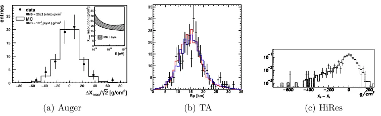
resolution obtained with data and MC stereo events has to be consistent if the detector simulation is working correctly. Figure10(a) shows the consistency of theXmax resolution obtained using data and
]
2
[g/cm 2 /
max
X ∆
−80 −60 −40 −20 0 20 40 60 80
entries
0 5 10 15 20 25
data
2
2 (stat.) g/cm ± RMS = 20
MC
2
(syst.) g/cm
+2 −1
RMS = 19
E [eV]
18
10 1019 1020
]
2
resolution [g/cm
max
X
0 5 10 15 20 25 30 35
sys. ± MC
(a) Auger
Rp [km]
0 5 10 15 20 25 30 35
0 5 10 15 20 25 30 35
(b) TA (c) HiRes
Figure 10. Validating the detector MC simulations. (a) AugerXmaxdifference of stereo events for data and MC. TheXmaxresolution is displayed as a function of energy in the inset. (b) TARpdistribution for data (black points) and MC (solid lines). The red and blue lines are for QGSJet-II proton and iron composition. (c) Difference between HiRes-II (XI I) and HiRes-I (XI)Xmaxfor HiRes stereo data (points) overlaid with QGSJet-II proton Monte Carlo calculations.
6.2 HiRes and TA
For the TA and HiRes approach, the detector MC simulations are used to estimate the expectedXmax
distributions after considering the detector effects. These expectations are estimated for different cosmic ray primaries. Then, the expected and observed Xmax distributions are compared to infer the average
cosmic ray composition.
Figure10(b) shows theRpdistribution for TA data and for MC calculations. Figure10(c) shows the
Xmaxdifference between HiRes-II (XI I) and HiRes-I (XI) for HiRes stereo data (points) overlaid with
QGSJet-II proton Monte Carlo calculations. The asymmetry is caused by HiRes-I covering only half the range in elevation angle. The Gaussian width of the peak is 44 g/cm2, setting an upper limit of 31 g/cm2
for the HiRes-IIXmaxresolution. Monte Carlo studies indicate that the actual HiRes-IIXmaxresolution
is better than 25 g/cm2over most of the HiRes energy range.
7. COMPARISON OFXMAXRESULTS FROM DIFFERENT EXPERIMENTS
In order to make sensible comparisons between experiments, we have used the observedXmaxvalues
to infer the average logarithmic mass,lnA, using.
lnA = Xmaxp− Xmaxdata Xmaxp− XmaxFe
ln 56, (2)
Similarly, one can transform Xmaxmeas into lnA by replacing Xmax withXmaxmeas in this equation
although this is only correct as a first order approximation. This is becauseXmaxmeasdoes not correlate
linearly withlnAasXmaxdoes [2].
When we transformed the measuredXmax into lnA, we used the expected Xmax values for
proton and iron obtained directly from Conex simulations. On the other hand, when we transformed the measuredXmeas
maxvalues, we used the expectedXmeasmax values for proton and iron extracted from the
simulation including the detector.
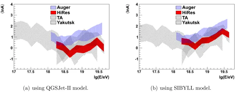
Figure 11shows the lnA estimated using the QGSJet-II and SIBYLL interaction models. The shaded regions indicate the range of the corresponding systematic uncertainties that were propagated from the systematic uncertainties in Xmax (12 g/cm2 for Auger and TA, 20 g/cm2 for Yakutsk, and
6 g/cm2for HiRes).
HiRes quotes systematics broken down into a 3.4 g/cm2 shift in the mean and an uncertainty of
(a) using QGSJet-II model. (b) using SIBYLL model.
Figure 11. Comparing the average composition (lnA) estimated using Auger, HiRes, TA and Yakutsk data. The shaded regions correspond to the systematic uncertainty ranges. To infer the average composition fromXmax, QGSJet-II and SIBYLL models have been used.
the two HiRes uncertainties into a single number by adding in quadrature the uncertainty in the mean and the shift due to a 1variation in slope over 1.6 decades of energy.
All the systematic uncertainties (on the measured Xmax) used in this work correspond to each
experiment’s quoted value. This working group has not attempted to validate those values.
At ultra-high energies, the Auger data suggest a largerlnAthan all other experiments. The Auger results are consistent within systematic uncertainties with TA and Yakutsk, but not fully consistent with HiRes. HiRes is compatible with the Auger data only at energies below 1018.5eV when using QGSJet-II (Fig.11(a)), and when using SIBYLL model, Auger and HiRes become compatible within a larger energy range (Fig.11(b)).
Comparing Figs.11(a) and11(b) we find that the level of incompatibility between Auger and HiRes data depends on the model used to interpret theXmaxobservations. Different models predict different
ranges ofXmaxvalues for proton and iron cosmic rays, and depending on how these predictions compare
with the range ofXmax values that could be inside the FOV of the detector, theXmeasmax(observed by
HiRes) could be more or less different to the intrinsicXmax, changing the interpretation ofXmeasmax.
The HiRes results are compatible in every way with the interpretation that the composition is light, i.e. lighter than the CNO group of elements. The AugerXmaxand RMS(Xmax) results do not allow this
interpretation.
Figure2shows that theXmaxobserved by Auger and theXmeasmaxobserved by HiRes and TA are
similar. Is there any physical reason that theXmaxfor Auger and theXmeasmaxfor HiRes and TA are
all similar, or is it just coincidence?. A direct way of checking the Auger and HiRes/TA compatibility would be to simulate a hypothetical composition which had the sameXmaxdistributions as observed by
Auger. Then this composition would be propagated through the HiRes and TA detector simulations and the expectedXmeas
max computed. So, we could compare directly the expected and observedXmeasmaxto
evaluate the compatibility of the Auger and HiRes/TA observations (this is work in progress).
We have also evaluated how the average logarithmic mass estimated by the experiments evolves as a function of energy. Currently there are two different models suggested by the Auger and HiRes collaborations. The Xmax and RMS(Xmax) observed by the Auger experiment suggest that the
composition might be becoming lighter with energy up to 1018.3eV, and heavier above this energy.
On the contrary, the Xmax and RMS(Xmax) observed by the HiRes experiment is consistent with a
Table 2. Fitting a horizontal line to thelnAas a function of energy.
Auger HiRes TA Yakutsk
ConstantlnA 1.11±0.03 0.6±0.1 0.8±0.2 0.3±0.2
2/ndf 133.6/10 4.4/7 9.8/7 7.7/7
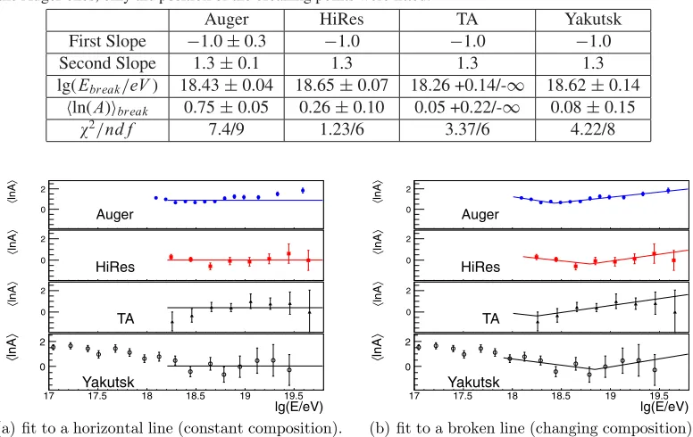
Table 3. Fitting a broken line to thelnAas a function of energy. For HiRes, TA and Yakutsk the slopes were fixed to the Auger ones, only the position of the breaking points were fitted.
Auger HiRes TA Yakutsk
First Slope −1.0±0.3 −1.0 −1.0 −1.0
Second Slope 1.3±0.1 1.3 1.3 1.3
lg(Ebreak/eV) 18.43±0.04 18.65±0.07 18.26 +0.14/-∞ 18.62±0.14
ln(A)break 0.75±0.05 0.26±0.10 0.05 +0.22/-∞ 0.08±0.15
2/ndf 7.4/9 1.23/6 3.37/6 4.22/8
17 17 5 18 18 5 19 19 5
〉
lnA
〈
0 2
Auger
17 17 5 18 18 5 19 19 5
〉
lnA
〈
0 2
HiRes
17 17 5 18 18 5 19 19 5
〉
lnA
〈
0 2
TA
lg(E/eV)
17 17.5 18 18.5 19 19.5
〉
lnA
〈
0 2
Yakutsk
(a) fit to a horizontal line (constant composition).
17 17 5 18 18 5 19 19 5
〉
lnA
〈
0 2
Auger
17 17 5 18 18 5 19 19 5
〉
lnA
〈
0 2
HiRes
17 17 5 18 18 5 19 19 5
〉
lnA
〈
0 2
TA
lg(E/eV)
17 17.5 18 18.5 19 19.5
〉
lnA
〈
0 2
Yakutsk
(b) fit to a broken line (changing composition).
Figure 12. Evaluation of the average composition (lnA) estimated using SIBYLL as a function of energy. Two composition models are evaluated, a constant composition (as suggested by HiRes and TA) and a changing composition with a break (as suggested by Auger). The results of the fits are summarized in Tables2and3.
Figure 12(a) shows the test of the HiRes model (a fit to a horizontal line). A horizontal line means constant composition in this plot. The large 2/ndf resulting from the fit of the Auger data (2/ndf =137/10) indicates that Auger data does not favor a constant composition model, but all
other experiments have2/ndf values embracing the constant composition model (see Table2).
Figure12(b) shows the test of the Auger model (a fit to a broken line). The fitted parameters are only the energy andlnAvalues at which the lines break. The slopes before and after the breaking point are fixed to the results of the Auger fit. The 2/ndf values for these fits are small. However, the Auger
energy andlnAfor the break point is not statistically compatible with the break points fitted by HiRes, TA or Yakutsk (see Table3). Further, studies (exploring the effect of different interaction models) and more statistics in the Northern Hemisphere are required to establish the level of compatibility between Southern and Northern Hemispheres.
8. OTHER OBSERVATIONS SENSITIVE TO MASS COMPOSITION
Apart fromXmaxobservations, other shower observables can also provide information of the average
lg(E/eV)
17 17.5 18 18.5 19 19.5 20
〉
lnA
〈
-2 -1 0 1 2 3 4
QGSJetII
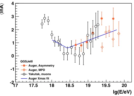
Auger, Asymmetry Auger, MPD Yakutsk, muons Auger Xmax fit
Figure 13. Average composition estimated using other (other thanXmax) shower observables. Open circles are using muon detectors from the Yakutsk experiment [5], solid circles use the observed shower asymmetries around the core with the Auger SD [21], and open crosses are using the estimated muon production depth maximum with the Auger SD.
shower core, and to estimate the muon production depth (MPD) maximum. These observations together with the assistance of Monte Carlo simulations of the detector and hadronic interaction models provide measurements of the average composition (lnA).
Figure13shows the average composition as a function of energy estimated using the muon detectors from the Yakutsk experiment, and the Auger ground array. For comparison purposes we have also included the broken lines fitted to the composition estimated using theXmaxobservations from Auger.
For all these estimates of the average composition the model QGSJet-II has been used.
Despite some systematic difference between measurements from AugerXmaxand Yakutsk muons,
both observations suggest that the composition becomes lighter up to about 1018.5eV and then it becomes heavier again above this energy. Measurements from Auger asymmetries also suggest that the composition becomes heavier above 1018.5eV. Measurements from Auger MPD only expand within
a narrow energy range, and they do not provide much information regarding the evolution of the composition as a function of energy.
9. DISCUSSION
When comparing thelnA values estimated from theXmax observations, results from Auger, TA
and Yakutsk are compatible within systematic uncertainties. TA and Yakutsk are also compatible with HiRes. However, Auger and HiRes are not fully compatible within systematic uncertainties.
As shown in Section 7, the level of compatibility between Auger and HiRes (the two highest-statistics observatories) depends on the particular interaction model used to interpret the Xmax
observations. Further experimental data on the high-energy hadronic interactions, e.g. from the LHC [25], would help to refine the current composition picture.
We need more statistics in the Northern Hemisphere (about 3 times the current statistics) in order to provide a conclusive statement to whether or not the composition is changing with energy in this Hemisphere. The current data, while completely consistent with a constant light composition, cannot definitively exclude a changing composition as suggested by Auger. More statistics are also necessary to establish whether there is indeed a difference in the RMS(Xmax) at higher energies between Auger
In the Northern Hemisphere HiRes has stopped data taking in 2006, however the hybrid TA observatory with a surface area of approximately 800 km2 will be acquiring additional data for the next several years at least.
Figure13showslnAmeasurements as a function of energy using different techniques. Despite the systematic differences, the measurements suggest a composition getting lighter at energies up to about 1018.5eV and a composition getting heavier above this energy. The systematic differences
between different type of measurements are very sensitive to the particular interaction model used for the interpretation. We showed the results for model QGSJet-II (in Fig.13), because all experiments had results available using this model.
References
[1] y J. Abraham et al. [Pierre Auger Coll.], Phys. Rev. Lett. 104 (2010) 091101 [2] L. Cazon and R. Ulrich. arXiv:1203.1781
[3] R. Abbasi et al. [HiRes Coll.], Phys. Rev. Lett. 104 (2010) 161101 [4] C. Jui et al. [TA Coll.], Proc. APS DPF Meeting arXiv:1110.0133 [5] L.G. Dedenko et al. J. Phys. G: Nucl. Part. Phys. 39 (2012) 095202 [6] J. Abraham et al., [Pierre Auger Coll.], NIM A 523 (2004) 50 [7] J. Abraham et al., [Pierre Auger Coll.], NIM A 620 (2010) 227 [8] R. U. Abbasi et al., Astropart. Phys. 23 (2005) 157
[9] H. Tokuno et al., NIM A 676 (2012) 54-65, and NIM A 689 (2012) 87 [10] M. Unger [Pierre Auger Coll.], Nucl. Phys. B, Proc. Suppl. 190 (2009) 240
[11] J. Bellido [Pierre Auger Coll.], Proc. XXth Rencontres de Blois (2009), arXiv:0901.3389 [12] D. Heck and J. Knapp, Forschungszentrum Karlsruhe, Tech. Report, (2001)
[13] N. N. Kalmykov and S. S. Ostapchenko, Phys. At. Nucl. 56 (1993) 346 [14] S. Ostapchenko, Nucl. Phys. B, Proc. Suppl. 151, 143 (2006)
[15] R. Fletcher et al., Phys. Rev. D 50 (1994) 5710
[16] R. Engel et al., in Proc. 26th Intl. Cosmic Ray Conference, Salt Lake City, Utah, (1999) [17] S.P. Knurenko et al., Proc. 27th ICRC, Hamburg 1 (2001), 157
[18] A.M. Hillas, J.R. Patterson. J.Phys.G:Nucl.Phys. 9 (1983), 323 [19] P. Facal for the Pierre Auger Coll. ICRC 2011, arXiv:1107.4804 [20] E.G. Berezhko et al. Astroparticle Physics 36 (2012) 31
[21] D. Garcia-Pinto for the Pierre Auger Coll. ICRC 2011, arXiv:1107.4804 [22] Energy spectrum working group report, this meeting
[23] J. Abraham et al. [Pierre Auger Coll.], Phys. Lett. B 685 (2010) 239 [24] V. de Souza for the Pierre Auger Coll. this meeting