Stochastic Control Foundations Of Autonomous Behavior

(1)

University of Pennsylvania

ScholarlyCommons

Publicly Accessible Penn Dissertations

2018

Stochastic Control Foundations Of Autonomous

Behavior

Santiago Paternain

University of Pennsylvania, spater@seas.upenn.edu

Follow this and additional works at:

https://repository.upenn.edu/edissertations

Part of the

Engineering Commons

This paper is posted at ScholarlyCommons.https://repository.upenn.edu/edissertations/3170 For more information, please contactrepository@pobox.upenn.edu.

Recommended Citation

Paternain, Santiago, "Stochastic Control Foundations Of Autonomous Behavior" (2018).Publicly Accessible Penn Dissertations. 3170.

(2)

Stochastic Control Foundations Of Autonomous Behavior

Abstract

The goal of this thesis is to develop a mathematical framework for autonomous behavior. We begin by describing a minimum notion of autonomy, understood as the ability that an agent operating in a complex space has to satisfy in the long run a set of constraints imposed by the environment of which the agent does not have information a priori. In particular, we care about endowing agents with greedy algorithms to solve problems of the form previously described. Although autonomous behavior will require logic reasoning, the goal is to understand what is the most complex autonomous behavior that can be achieved through greedy algorithms. Being able to extend the class of problems that can be solved with these simple algorithms can allow to free the logic of the system and to focus it towards high-level reasoning and planning.

The second and third chapters of this thesis focus on the problem of designing gradient controllers that allow an agent to navigate towards the minimum of a convex potential in punctured spaces. Such problem is related to the problem of satisfying constraints since we can interpret each constraint as a separate potential that needs to be minimized. We solve this problem first in the case where the information about the potential and the obstacles is deterministic and complete and later, in Chapter \ref{chap_stochnf}, we consider the case where this information is only available from a stochastic model. In both cases, we derive sufficient conditions in which a Rimon-Koditschek artificial potential can be tuned into a navigation function and hence being able to solve the problem. These conditions relate the geometry of the potential of interest and the geometry of the obstacles.

Chapter \ref{chap_feasibility} considers the problem of satisfying a set of constraints when their temporal evolution is arbitrary. We show that an online version of a saddle point controller generates trajectories whose fit and regret are bounded by sublinear functions. These metrics are associated with online operation and they are analogous to feasibility and optimality in classic deterministic optimization. The fact that these quantities are bounded by sublinear functions suggests that the trajectories approach the optimal solution. Saddle points have the advantage of providing an intuition on the relative hardness of satisfying each constraint. The limit values of the multipliers are a measure of such relative difficulty, the larger the multiplier the larger is the cost in which one incurs if we try to tighten the corresponding constraint. In Chapter \ref{chap_counterfactuals} we exploit this property and modify the saddle point controller to deal with situations in which the problems of interest are not feasible. The modification of the algorithm allows us to identify which are the constraints that are harder to satisfy. This information can later be used by a high logic reasoning to modify the problem of interest to make it feasible.

Before concluding remarks and future work we devote our attention to the problem of non-myopic agents. In Chapter \ref{chap_rl} we consider the setting of reinforcement learning where the objective is to maximize the expected cumulative rewards that the agent gathers, i.e., the $Q$-function. We model the policy of the agent as a function in a Reproducing Kernel Hilbert Space since this class of functions has the advantage of being quite rich and allows us to compute policy gradients in a simple way. We present an unbiased estimator of the policy gradient that can be constructed in finite time and we establish convergence of the stochastic gradient policy ascent to a function that is a critical point of the $Q$-function.

Degree Type

(3)

Degree Name

Doctor of Philosophy (PhD)

Graduate Group

Electrical & Systems Engineering

First Advisor

Alejandro Ribeiro

Subject Categories

(4)

STOCHASTIC CONTROL FOUNDATIONS OF AUTONOMOUS BEHAVIOR Santiago Paternain

A DISSERTATION in

Electrical and Systems Engineering

Presented to the Faculties of the University of Pennsylvania in Partial Fulfillment of the Requirements for the

Degree of Doctor of Philosophy 2018

Supervisor of Dissertation

Alejandro Ribeiro, Rosenbluth Associate Professor of Electrical and Systems Engineering

Graduate Group Chairperson

Alejandro Ribeiro, Rosenbluth Associate Professor of Electrical and Systems Engineering

Dissertation Committee

(5)

STOCHASTIC CONTROL FOUNDATIONS OF AUTONOMOUS BEHAVIOR

COPYRIGHT

2018

(6)

Acknowledgments

The years that I spent as a Ph.D. student were some of the most valuables in my life for both professional and personal reasons. I am extremely grateful to be able to appreciate and acknowledge the influence of my advisor, collaborators and friends on writing this thesis.

First and foremost, I would like to express my sincere gratitude to my advisor Prof. Alejandro Ribeiro for opening me the doors of his laboratory. This thesis would not have been possible without his comments, suggestions and support. I want to thank him for the significant impact in shaping my career but also my personality. It has been my great pleasure to have the privilege of being his student. Alejandro has positively influenced my life at a stage that I will always regards fondly and for that reason I am grateful as well.

I would like to further thank Dr. Daniel E. Koditschek, Dr. Manfred Morari and Dr. Alec Koppel, for agreeing to serve in my doctoral committee and for giving me the opportunity to collaborate with them in different projects. Although not all of them resulted in technical content for this thesis, their positive impact on my research experience which led to writing this thesis is invaluable.

Writing this thesis will not have been possible without the joint effort of my collabora-tors. I would like to thank Dr. Juan Andr´es Bazerque from the Universidad de la Rep´ublica in Uruguay, and Austin Small. Over the course of my PhD, I’ve been fortunate to make some meaningful friendships that have strengthened my research purpose. Specifically, I benefited greatly from working closely with Dr. Aryan Mokthari and Mahyar Fazlyab.

I would also like to extend a deep sense of gratitude to my friends in the laboratory to which I belonged over the past five years. I would especially like to mention here Luiz Chamon, Fernando Gama, Dr. Miguel Calvo-Fullana and Markos Epitropou. Your support from a personal standpoint and frienship made me feel at home. I’d would also like to mention other friends in graduate school with me, whose presence has made the whole process much more enjoyable, and included but not limited to: Ceyhun Eksin, Santiago Segarra, Weiyu Huang, Mark Eisen, Shi-Ling Phuong, Ekaterina Tolstaya, Harshat Kumar, Luana Ruiz, Maria Pfiefer Alp Aydinoglu and Dr. Antonio Garc´ıa-Marques.

(7)

well to my friends back home in Uruguay. Special thanks to my parents, Pilar and Miguel. “Thank you” is insufficient for your consistent support, limitless sacrifices and indescribable love. To my grandmother Olga, cousins, uncles and aunts. Last but not least, to Mercedes. Thank you for always being there for me and for believing in me more than myself. This thesis would not have been written without your unconditional love and support. Dedicating this thesis to you is the least I could do to acknowledge your role in writing this thesis and appreciate your kindness and love.

(8)

ABSTRACT

STOCHASTIC CONTROL FOUNDATIONS OF AUTONOMOUS BEHAVIOR Santiago Paternain

Alejandro Ribeiro

The goal of this thesis is to develop a mathematical framework for autonomous behavior. We begin by describing a minimum notion of autonomy, understood as the ability that an agent operating in a complex space has to satisfy in the long run a set of constraints imposed by the environment of which the agent does not have information a priori. In particular, we care about endowing agents with greedy algorithms to solve problems of the form previously described. Although autonomous behavior will require logic reasoning, the goal is to understand what is the most complex autonomous behavior that can be achieved through greedy algorithms. Being able to extend the class of problems that can be solved with these simple algorithms can allow to free the logic of the system and to focus it towards high-level reasoning and planning.

The second and third chapters of this thesis focus on the problem of designing gradient controllers that allow an agent to navigate towards the minimum of a convex potential in punctured spaces. Such problem is related to the problem of satisfying constraints since we can interpret each constraint as a separate potential that needs to be minimized. We solve this problem first in the case where the information about the potential and the obstacles is deterministic and complete and later, in Chapter 3, we consider the case where this information is only available from a stochastic model. In both cases, we derive sufficient conditions in which a Rimon-Koditschek artificial potential can be tuned into a navigation function and hence being able to solve the problem. These conditions relate the geometry of the potential of interest and the geometry of the obstacles.

(9)

the algorithm allows us to identify which are the constraints that are harder to satisfy. This information can later be used by a high logic reasoning to modify the problem of interest to make it feasible.

Before concluding remarks and future work we devote our attention to the problem of non-myopic agents. In Chapter 6 we consider the setting of reinforcement learning where the objective is to maximize the expected cumulative rewards that the agent gathers, i.e., the Q-function. We model the policy of the agent as a function in a Reproducing Kernel Hilbert Space since this class of functions has the advantage of being quite rich and allows us to compute policy gradients in a simple way. We present an unbiased estimator of the policy gradient that can be constructed in finite time and we establish convergence of the stochastic gradient policy ascent to a function that is a critical point of theQ-function. 1

1_{Work presented in this thesis has been published and submitted for review to IEEE Transactions on}

(10)

List of Tables

2.2 Percentage of successful simulations when the condition guaranteeing thatϕk

(15)

List of Figures

2.1 The artificial potential fails to be a navigation function fork= 2 andk= 10 when (2.23) is violated and the direction defined by the center of the obstacle and the goal is collinear to the direction of the eigenvector corresponding to the smallest eigenvalue of the Hessian of the objective function. . . 22 2.2 For k= 2 the artificial potential is a navigation function even though (2.23)

is violated but the direction defined by the center of the obstacle and the objective is perpendicular to the direction of the eigenvector corresponding to the smallest eigenvalue of the Hessian of the objective function. Recall that when those directions are collinear (Figures 2.1(a) and 2.1(b)), the potential

ϕk fails to be a navigation function. . . 23

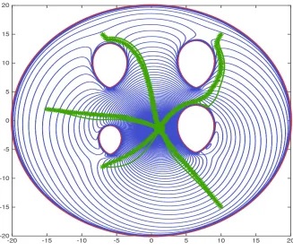
2.3 Trajectories for different initial conditions in an elliptical world inR3. As per

Theorem 3 and 4 the trajectory converges to the minimum of the objective function while avoiding the obstacles. In this example we have d= 10 and

k= 25. . . 33 2.4 Navigation function in an Egg shaped world. As predicted by Theorem 4

the trajectory arising from (2.36) converges to the minimum of the objective functionf0 while avoiding the obstacles. . . 34

2.5 In orange we observe the trajectory arising from the system without dynamics (cf., (2.34)). In green we observe trajectories arising from the system (2.40) when we the control law (2.41) is applied. The trajectory in dark green has a larger damping constant than the trajectory in light green and therefore it is closer to the trajectory of the system without dynamics. . . 36 2.6 In green we depict the trajectories of the kinematic differential drive robot

(2.42) , when the control law is given by (2.45) and (2.46). In orange we depict the trajectories of the dynamic differential drive robot (2.42) and (2.43) , when the control law is given by (2.47) and (2.48). In both cases we select

(16)

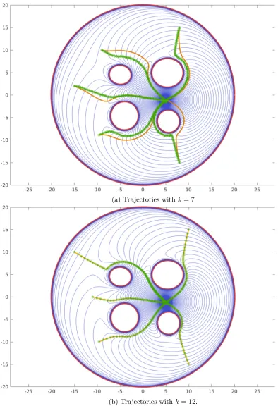
3.1 The trajectories resulting of the navigation function approach – solid line– and its stochastic approximation given in (3.10) –stars–succeed in driving the agent to the goal configuration for five different initial positions as expected in virtue of Theorem 6. We observe that for the same world (cf., Figures 3.1(a) and 3.1(b)) the larger the order parameter k is, the closer the trajec-tory resulting from stochastic approximation is to the trajectrajec-tory resulting of descending along the gradient of the navigation function (2.17). . . 56 3.2 The trajectories resulting of the navigation function approach with k= 15 –

solid line– and its stochastic approximation given in (3.10) –stars–succeed in driving the agent to the goal configuration for five different initial positions as expected in virtue of Theorem 6. . . 57 3.3 Estimation of the obstacles by the hallucinated osculating circle for a

partic-ular position in the free space with exact and stochastic information. Obsta-cles are sensed if di(x)<7. Noise is Gaussian, additive, mean zero and with varianceσdi =σRi =σni =di(x)/10. . . 58

3.4 Evolution of the distance to the goal in a world with elliptical obstacles. We set the order parameter of the navigation function to k = 12, and the step size to satisfy Assumption 5 with the following parameters η0 = 1×10−7,

ζ = 5×10−5. . . 59 3.5 Trajectories resulting of following the negative gradient of the logarithmic

barrier given in (3.37) for k = 10 in an elliptical world. The trajectories resulting from the update (3.10) succeed in driving the agent to the goal con-figuration for five different initial positions as expected in virtue of Theorem 7. . . 62 4.1 Block diagram of the saddle point controller. Once that actionx(t) is selected

at time t, we measure the corresponding values of f(t, x(t)), fx(t, x(t)) and f0,x(t, x(t)). This information is fed to the two feedback loops. The action

loop defines the descent direction by computing weighted averages of the subgradients fx(t, x(t)) and f0,x(t, x(t)). The multiplier loop uses f(t, x(t))

to update the corresponding weights. . . 78 4.2 Path of the sheep and the shepherd for the feasibility-only problem (Section

(17)

4.3 Relationship between the instantaneous value of the constraints and their corresponding multipliers for the feasibility-only problem (Section 4.5.1). At the times in which the value of a constraint is positive, its corresponding mul-tiplier increases. When the value of the mulmul-tipliers is large enough a decrease of the value of the constraint function is observed. Once the constraint func-tion is negative the corresponding multiplier decreases until it reaches zero.

. . . 92 4.4 FitFT for two different controller gains in the feasibility-only problem

(Sec-tion 4.5.1). Fit is bounded in both cases as predicted by Theorem 9. As is also predicted by Theorem 9, the larger the value of the gain K the smaller the bound on the fit of the shepherd’s trajectory. . . 93 4.5 FitF_T for the preferred sheep problem (Section 4.5.2) when the gain of the

saddle point controller is set to be K = 50. As predicted by Theorem 10 the trajectory is feasible since the fit is bounded, and, in fact, appears to be strongly feasible. Since the subgradient of the objective function is the same as the subgradient of the first constrain the fit is smaller than in the pure feasibility problem (cf., Figure 4.4). . . 95 4.6 RegretR_T for the preferred sheep problem (Section 4.5.2) when the gain of

the saddle point controller is set to be K = 50. The trajectory is strongly optimal, as predicted by Theorem 10, since the regret is bounded by a con-stant. The initial increment in the regret is due to the fact that the shepherd starts away from the first sheep while in the optimal offline trajectory would start close to it. . . 96 4.7 Path of the sheep and the shepherd for the minimum acceleration problem

(Section 4.5.3) when the gain of the saddle point controller is set to be K = 50. Observe that the shepherd path – in red – is not as close to the path of the sheep as in Figure 4.2. This is reasonable because the objective function and the constraints push the shepherd in different directions. . . 97 4.8 FitF_T for the minimum acceleration problem (Section 4.5.3) when the gain

(18)

4.9 Regret R_T for the minimum acceleration problem (Section 4.5.3) when the gain of the saddle point controller is set to be K = 50. The trajectory is strongly optimal as predicted by Theorem 10. Observe that regret is negative due to the fact that the agent is allowed to select different actions at different times as opposed to the clairvoyant player that is allowed to select a fixed action. . . 99 4.10 Path of the sheep and the shepherd for preferred sheep problem when

satu-rated fit is considered (Section 4.5.4) and the gain of the saddle point con-troller is set to be K= 50. The shepherd succeed in following the herd since its path – in red – is close to the path of all sheep. . . 100 4.11 Saturated fit Fsat

T for the preferred sheep problem (Section 4.5.4) when the

gain of the saddle point controller is set to K = 50. Since the saturated fit grows sublinearly in accordance with Corollary 6, the trajectory is feasible. 101 4.12 RegretRT for the preferred sheep problem when saturated fit is considered

(Section 4.5.4)and the gain of the saddle point controller is set to beK = 50. The regret is bounded as predicted by Corollary 6 and therefore the trajectory is strongly optimal. Notice that regret in this case is identical to regret in the preferred sheep problem when regular fit is considered (cf., Figure 4.6). 102 5.1 We observe the evolution of the slacks for the solutions of the dynamical

system (5.9)–(5.11). In blue and red we observe the evolution of the slacks

µ₁ and µ₂ corresponding to the constraints fi(x) = kx−xik2, with x1 =

[−3,−1] andx2= [−3,1]. In yellow we observe the slackµ3for the constraint

with centerx3= [3,0]. Because the centers of the first two solutions are closer

between them as compared to the third center. It is not surprising that the slack required to satisfy those constraints is smaller. . . 122 6.1 Numerical gradient via stochastic approximation; (left) two-sample

approxi-mation, (right) full-dimension. Red levels represents higher values ofQ(s, a;h).138 6.2 Result of representative run of Algorithm 5 over 50,000 Continuous Mountain

(19)

Chapter 1 Introduction

Systems capable of exhibiting autonomous behavior and that are able to perform complex tasks without human assistance are of importance, especially when deployed in environments that are dangerous for humans, like collapsed buildings or zones with toxic or chemical waste spills. Such systems can also be used in theory to perform complex medical procedures or to simplify human tasks in domestic applications and transportation, and therefore it is not surprising that creating autonomous systems has been an actively pursued goal.

While there are many different perspectives of autonomy, a minimal definition is that an agent exhibits autonomous behavior if it can survive when deployed in a complex en-vironment about which there is no information available a priori. Mathematically, we can think of the environment as presenting the agent with a set of unknown functions and of the agent as selecting an action that results in an equal number of payoffs. The agent has the ability to sense the outcome of his actions and must select actions based on a policy that makes the cumulative reward obtained along its trajectory close to a certain value. As a reference problem that can be formulated in this language, consider a drone that is to be positioned within range of a number of targets whose positions are unknown. The drone has to do so with an energy budget and the space in which this task is to be accomplished may be an open field or a wooded area. The drone survives in an environment if it is endowed with an algorithm that allows it to place himself within range of the targets while satisfying the energy constraint. We say that the drone exhibits autonomous behavior if it can satisfy these constraints irrespectively of the environment in which it is deployed – i.e., irrespectively of the position and number of targets and of whether the environment is open or wooded.

(20)

stochastic control rules can solve a bigger class of problems than currently considered feasible and, as a consequence of sorts, that the interface between low-level greedy rules and high-level logical reasoning have to take a different form. The goal of this thesis is to expand the foundations of stochastic gradient control to incorporate these problems into the class of problems for which greedy algorithms have provable convergence certificates and to exploit this expansion to propose novel methodologies to interface between low-level control and high-level algorithmic reasoning.

To provide a more detailed explanation we adopt a taxonomy that classifies problems with respect to three main properties, the complexity of the space in which the agent is deployed, the amount of information that is available prior to deployment and the time horizon of the operation. The (configuration) spaces in which the agent is deployed can be assumed to be open, punctured or complex. An open environment is one in which there are no restrictions in the configuration space, a punctured space is one that is characterized by the presence of compact obstacles homeomorphic to a point, and a complex environment is one in which the configuration space has an arbitrary shape. The information available a priori is classified as complete, stochastic, viability, or none. Having complete information means that the environment and the constraints to be satisfied are known. Stochastic information means that a probabilistic model of the world is available. Viability means that no information is given except for the knowledge that there is a strategy that would permit satisfaction of all the constraints that specify the environment. In the extreme case, not even this information is available and the agent has to discover whether the environment is viable or not. If the environment is not viable, an autonomous agent has to be able to fall back into a laxer notion of survivability. Finally, the time horizon of the operation distinguishes between myopic operation, where the agent tries to solve the problem for the current time instance, without taking into account the consequences that such actions could have in the future, and farsighted operation, where the agent might make decisions that in the short term are not optimal, but they imply better rewards in the future.

(21)

model of the environment is given a priori, the situation is much different but the solution methodology is about the same. If the constraints and their gradients can be estimated lo-cally without bias, a stochastic saddle point controller can be proven to converge to a point at which the constraints are satisfied [65]. Do notice that in both cases we must require the existence of a point at which the constraints are satisfied and that the functions that define the environment are convex. This latter condition is not restrictive if we assume that the agent is equipped with local sensors because in that case, a local solution is all that we can hope for.

While greedy saddle point controllers and their stochastic approximations can solve myopic problems in open environments when information is stochastic, this is not enough for the minimal notion of autonomous behavior previously described. Problems in complex environments are addressed with path planning tools which, in the case of stochastic or viability specifications, are coupled with a preliminary mapping stage. Although there are many different specific path planning methods, they can be broadly considered as a decomposition approach because their overall goal is to separate trajectories in complex environment into mesoscale pieces that are locally open and can be planned using tools that work well in open environments. Problems in which it is necessary to discover a measure of what sort of constraints can be satisfied in the environment are addressed heuristically through trial and error. The second drawback about greedy saddle point controllers is that they can only solve problems where the costs are myopic. This is, they offer a solution for an optimization problem without taking into account the rewards –or payoffs– collected along the trajectory. Operating in a regime where one looks at the future is part of the requirements for autonomy. This means, that it is justified to select an action at a given time that results in a low payoff, but it places the system in a state where better rewards can be collected in the long run. Say for instance that an agent requires to place itself to a given distance from a set of targets but it is running out of battery. A myopic controller might prioritize to follow the targets to maximize the payoff without recharging the battery, and thus failing to complete the mission in the future. On the other hand, stopping for re-charging might produce smaller rewards in the short term, but allows the agent to be in a state – high battery level– that allows him in the future to re-position close to the targets for a longer time.

(22)

1.1 Main Contributions

We next detail the thrusts motivated in the previous paragraphs by outlining the work that is presented in this thesis and the particular questions that we address in each chapter.

1.1.1 Navigation functions in punctured spaces.

In the previous paragraphs the motivation of designing algorithms that allow a mobile robot to avoid obstacles has been presented. Many efforts have been made in this direction in situations in which a desired configuration xdis provided explicitly to the agent. Formally,

obstacles are defined as open setsO_i in the workspace. The set of valid configurations con-sist of the set difference of the workspace and the obstacles and its termed the free space. The objective is then to converge to xd while remaining on the free space at all times. A

way of greedily solving this problem is through artificial potentials, see e.g. [38, 49, 131]. These potentials are a superposition of an attractive potential – having its minimum at the desired configuration– and repulsive potentials at the obstacles – taking maximum value at their boundary. In some of these constructions convergence to xd cannot be ensured

because of the presence of local minima due to the superposition of several potentials. However, the construction in [57] ensures convergence to the desired point from almost all initial conditions, in a space with spherical obstacles. The potential build in [57] has some defining properties that ensures convergence to xd and obstacle avoidance. These are that the potential has a unique minimum that coincides with xd, that all critical points are

non degenerate and that the maximum of the potential coincides with the boundary of the obstacles. A potential satisfying these properties define what the authors call a navigation function. In [57] it is also shown that navigation from all initial positions is not possible, and therefore almost sure navigation is the best that one can achieve. The ideas in [57] have been extended to generic star obstacles in [106], yet to do so, a diffeomorphism mapping the world into a spherical world needs to be constructed and to do so, complete information of the environment is required beforehand. The first advantage of this framework compared to some of the other path planning algorithms – such as visibility graphs [81] or cell de-composition [22, 23, 69, 73] – is that it does not require the use of logic and can, therefore, be programmed at a very low level. This can release the logic of these simple task and be available to develop some high level reasoning. A second advantage of gradient descent like algorithms is that they can be easily generalized to systems with intrinsic dynamics. Other path planning algorithms do not take into account the dynamics of the system and therefore may provide trajectories that are not feasible for the robot.

(23)

typically the result of knowing the desired destinationxdbeforehand. In other applications,

however, it is more reasonable to have the desired configuration given as the solution of an optimization problem. As a reference example, think about a robot that is trying to reach the top of a hill. It is more reasonable to assume that the agent can sense its way up the hill using, for instance, an Inertial Measurement Unit (IMU) instead of requiring the location of the top. Along the same lines, it might be of interest to be able the find the source of a given signal, for example, the source of a gas leak which might be expressed as the position for which the gas concentration is the highest. In this setting, it is not reasonable to assume that the positionxdis known and the agent needs to follow the gradient of the intensity of

the signal it receives to localize its source.

In Chapter 2 we generalize the artificial potentials from [57] to construct navigation functions in situations in which the attractive potential is not necessarily rotationally sym-metric. In particular, we provide sufficient conditions for the possibility of constructing navigation functions of the form in [57]. These conditions relate the geometry of the poten-tial with the geometry of the free-space and the intuition behind them are that the flatter the obstacles are with respect to the level curves of the attractive potential, the hardest it is to tune construct a navigation function.

1.1.2 Online observation of obstacles and environment.

The approach based on navigation functions requires some restrictive assumptions regarding the gradient and the value of the objective function being known exactly at each location. For instance, suppose that a terrestrial robot is trying to reach the top of a hill. The slope of the hill is estimated using measures from onboard accelerometers. These sensors provide noisy measure and hence the estimation cannot be exact. Likewise, it requires complete knowledge of the obstacles, when it is more reasonable to assume that obstacles that are far away from the current position should not influence the behavior of the agent. In addition, the knowledge of the obstacles is inferred using sensors, e.g. LIDARs, and in that sense, the estimates will be contaminated with measurement noise.

Measurements of the objective function f0(x) or its gradient ∇f0(x) can be used to

construct an estimator of the gradient of the objective function. This estimate is a random variable denoted by ˆ∇f0(xt, θt) which depends on the configuration of the agent at time t and on a random variable θt that accounts for measurement noise. If the estimate is unbiased it means that on average the estimate at a given location is equal to the gradient of the function at that point. Formally, it means that the expectation of the noisy gradient with respect to the noise is the gradient itself, i.e., Eθt

h

ˆ

∇f0(xt, θt) i

= ∇f0(xt). If we

(24)

probability one (see e.g [107]).

The first question to answer is how to use inexact information to build estimates of the obstacles. For instance, if obstacles are spherical, estimates of the radius and the distance to an obstacle are the minimum information required to avoid them. A naive approach could be to artificially enlarge the obstacles to take into account estimation errors. The insights obtained in the deterministic setting (cf., Chapter 2) suggest that the larger the obstacles and the closer they are to the desired position, make the navigation harder. This has also been observed in [35, 57]. Hence, the previous solution could be over conservative and yield unnecessary stiff trajectories and even make navigation impossible. A second issue to consider is that the navigation function framework relies upon the complete knowledge of the obstacles – shape, position, and size. It is clear that by considering a robot that senses the obstacles as it moves in the space this assumption must be dropped. This fact introduces a mismatch between local estimates the obstacle – obtained for instance by fitting an osculating circle at the closest point of the obstacle from the agent – and the true world. In Chapter 3 we show that if that said mismatch is not large as compared to the gradient of the navigation function, safe navigation to a neighborhood of the desired configuration is achieved from all initial positions with probability one.

1.1.3 Viability and strategic behavior

The third thrust is related to being able to perform tasks in environments that are time-varying, meaning that the objective functions or the constraints could change over time. In particular, we are interested in adversarial environments, where the change of the function at time t, is such that the action decided at time t−1 is the worst choice that we could have selected. To illustrate this idea we can think of the robot as playing a game against the environment. The game is as follows, at timet the agent is allowed to select an action to play at timet+ 1, based on the information of the function that he is trying to minimize at time t. The objective function now is a set of functions {f0,t(x), t∈N} of which the

agent only knows at time T the value of the functions f0,t(xt) for t= 0. . . T. Because of

the adversarial nature of the environment and the lack of information about the evolution of it, we cannot possibly expect that the agent minimizes the function f0,t at any time.

Therefore the success of an agent in this kind of environment is established through the idea of regret. Regret is the difference between the total loss in which the agent incurs and the loss in which a clairvoyant agent would have incurred if he was allowed to play always the same action. Formally, regret at timeT can be expressed as

R_T =

T

X

t=0

f0,t(xt)−min x∈_Rn

T

X

t=0

(25)

If the above quantity is large, having known the evolution of the system we could have chosen a strategy in which the cost incurred is smaller. In that sense, the above quantity measures how much we regret not having that information available. This framework was introduced first in [128] and it has been shown in [138] that an online version of gradient descent achieves regret bounded byO(√T). Having sublinear regret means that the action that we are selecting is approaching the optimal solution. Further works show that by changing the step size of the update can improve the bounds on regret. For instance, in [42] it is shown that online gradient descent with diminishing step size for strongly convex functions archives regret bounded by O(log(T)). In Chapter 4 we present a continuous time version of this problem and establish regret bounded by a constant. We can think of the problem of satisfying a set of constraint in an adversarial environment as well using a similar concept to that of regret named Fit. The latter is the total constraint violation in which an agent incurs

F_T =

Z T

0

f(t, x(t))dx. (1.2) This quantity measures – in the same sense that regret measures optimality– how far we are from satisfying the constraints. If there is an action that satisfies the constraints for all times, having known the evolution of the system we could determine this action and have a negative Fit. By having a total constraint violation that grows sublinearly gives the idea of approaching the action that is feasible for all times. In Chapter 4 it is shown that an online version of the algorithm by Arrow Hurwicz proposed in [4] achieves bounded fit irrespectively of the time horizon T. Furthermore, we show that if an optimality criterion is added regret is still bounded by a constant but the fit now is bounded by a function that grows asO(√T).

1.1.4 Price interfaces

(26)

through a saddle point algorithm it is easy to identify if the problem is not feasible, because the multipliers keep increasing. With this information the part of the system in charge of the logical reasoning has the information about which constraints should be modified to succeed on its goal or at least it has the information about which of the constraints does not allows him to perform a given task. For instance, let us consider the surveillance problem in which we are interested in tracking several obstacles. Suppose that there is no way of being close to all of the targets, then a mechanism to identify which one of the constraints is the hardest to satisfy can be used by the logical reasoning part of the system to decide a different policy. For instance it could change the problem of being at a given distance of all the targets for a new problem stated as being at a given distance of the target whose multipliers are bounded and adding an optimality criteria given by being as close as possible to the remaining targets. The problem of deciding the policy that must be accomplished is the task of the logical reasoning part of the system, and as discussed the information arising from the low level control is a fundamental piece of information to effectively chose the strategy to follow.

In Chapter 5 we propose a modification of the saddle point algorithm for both the deterministic setting and the setting where a probabilistic model of the constraints and the objective function is available to the agent. This modification introduces adaptive slack variables for each constraint and updates them by increasing its value if the corresponding multiplier is positive and decreases the value if the slacks grows too much. The algorithm is such that it converges to the primal-dual solution for a slack that is proportional to the dual variable. By analyzing the slacks, and the value of the multipliers, we get a relative measure of which constraints are harder to satisfy.

1.1.5 Non-myopic behavior

(27)

the policy that maximizes the expectation of the cumulative reward, also known as the

Q-function of the MDP. A solution to these problems can be found in the reinforcement learning literature. This is a model-free control framework for MDPs, where the transition probabilities from one state to next one are not known but the decision policy is based on the rewards obtained. When the state and action spaces are discrete, the solutions to these problems can be divided among those that learn theQ–function to then chose for any given state the action that maximizes the function [132] and those that attempt to directly learn the optimal policy by running gradient ascent in the space of policies [27, 120].

A major drawback of the previous algorithms for reinforcement learning is that they suffer from the curse of dimensionality, this is, the complexity of the problem scales ex-ponentially with the number of actions and states [37]. This is, in particular, the case of continuous spaces, where any reasonable discretization leads to a very large number of states and possible actions. Efforts to sidestep this issue assume that either theQ-function or the policy admits some parametrization [13, 119], or that it belongs to a Reproducing Kernel Hilbert Space (RKHS) [61, 71, 126]. The latter provides the ability to approximate functions using nonparametric functional representations. Although the structure of the space is determined by the choice of the kernel, the set of functions that can be represented is sufficiently rich to permit a good approximation of a large class of functions.

(28)

Chapter 2 Navigation Functions for Convex

Potentials in a Space with Convex

Obstacles

Given a convex potential in a space with convex obstacles, an artificial potential is used to navigate to the minimum of the natural potential while avoiding collisions. The artifi-cial potential combines the natural potential with potentials that repel the agent from the border of the obstacles. This is a popular approach to navigation problems because it can be implemented with spatially local information that is acquired during operation time. Artificial potentials can, however, have local minima that prevent navigation to the mini-mum of the natural potential. In this chapter we derive conditions that guarantee artificial potentials have a single minimum that is arbitrarily close to the minimum of the natural potential. The qualitative implication is that artificial potentials succeed when either the condition number– the ratio of the maximum over the minimum eigenvalue– of the Hessian of the natural potential is not large and the obstacles are not too flat or when the desti-nation is not close to the border of an obstacle. Numerical analyses explore the practical value of these theoretical conclusions.

2.1 Introduction

(29)

source of a specific signal can be used by mobile robots to perform complex missions such as environmental monitoring [92, 117], surveillance and reconnaissance [110], and search and rescue operations [64]. In all these scenarios the desired configuration is not available beforehand but a high level task is nonetheless well defined through the ability to sense the environment.

These task formulations can be abstracted by defining goals that minimize a convex potential, or equivalently, maximize a concave objective. The potential is unknown a priori but its values and, more importantly, its gradients can be estimated from sensory inputs. The gradient estimates derived from sensory data become inputs to a gradient controller that drives the robot to the potential’s minimum if it operates in an open convex environment, e.g [43, 122]. These gradient controllers are appealing not only because they exploit sensory information without needing an explicit target configuration, but also because of their simplicity and the fact that they operate using local information only.

In this chapter we consider cases where the configuration space is not convex because it includes a number of nonintersecting convex obstacles. The goal is to design a modified gradient controller that relies on local observations of the objective function and local obser-vations of the obstacles to drive the robot to the minimum of the potential while avoiding collisions. Both, objective function and obstacle observations are acquired at operation time. As a reference example think of navigation towards the top of a wooded hill. The hill is modeled as a concave potential and the trunks a set of nonintersecting convex punctures. The robot is equipped with an inertial measurement unit (IMU) providing the slope’s di-rectional derivative, a GPS to measure the current height and a lidar unit giving range and bearing to nearby physical obstacles [45, 46]. We then obtain local gradient measurement from the IMU, local height measurements from the GPS and local models of observed ob-stacles from the lidar unit and we want to design a controller that uses this spatially local information to drive the robot to the top of the hill.

A possible solution to this problem is available in the form of artificial potentials, which have been widely used in navigation problems, see e.g. [10,11,25,33–36,49–51,57,62,74,75,77, 78, 80, 91, 106, 109, 131]. The idea is to mix the attractive potential to the goal configuration with repulsive artificial fields that push the robot away from the obstacles. This combination of potentials is bound to yield a function with multiple critical points. However, we can attempt to design combinations in which all but one of the critical points are saddles with the remaining critical point being close to the minimum of the natural potential. If this is possible, a gradient controller that follows this artificial potential reaches the desired target destination while avoiding collisions with the obstacles for almost all initial conditions (see Section 2.2).

(30)

has been widely studied when the natural potential is rotationally symmetric. Koditschek-Rimon artificial potentials are a common alternative that has long been known to work for spherical quadratic potentials and spherical holes [57] and more recently generalized to focally admissible obstacles [35]. In the case of spherical worlds local constructions of these artificial potentials have been provided in [34]. Further relaxations to these restrictions rely on the use of diffeomorphisms that map more generic environments. Notable examples are Koditschek-Rimon potentials in star shaped worlds [105, 106] and artificial potentials based on harmonic functions for navigation of topological complex three dimensional spaces [77,78]. These efforts have proven successful but can be used only when the space is globally known because that information is needed to design a suitable diffeomorphism. Alternative solutions that are applicable without global knowledge of the environment are the use of polynomial navigation functions [74] for n-dimensional configuration spaces with spherical obstacles and [75] for 2-dimensional spaces with convex obstacles, as well as adaptations used for collision avoidance in multiagent systems [28, 109, 124].

Perhaps the most comprehensive development in terms of expanding the applicability of artificial potentials is done in [33, 35, 36]. This series of contributions reach the conclusion that Koditschek-Rimon potentials can be proven to have a unique minimum in spaces much more generic than those punctured by spherical holes. In particular it is possible to navigate any environment that is sufficiently curved. This is defined as situations in which the goals are sufficiently far apart from the borders of the obstacles as measured relative to their flatness. These ideas provides a substantive increase in the range of applicability of artificial potentials as they are shown to fail only when the obstacles are very flat or when the goal is very close to some obstacle border. These curvature conditions seems to be a fundamental requirement of the problem itself rather than of the solution proposed, since it is present as well in other navigation approaches such as navigation via separating hyperplanes [5–7].

(31)

not too flat. (ii) The distance from the obstacles’ borders to the minimum of the natural potential is large relative to the size of the obstacles. These conditions are compatible with the definition of sufficiently curved worlds in [33]. To gain further insight we consider the particular case of a space with ellipsoidal obstacles (Section 2.3.1). In this scenario the condition to avoid local minima is to have the minimum of the natural potential sufficiently separated from the border of all obstacles as measured by the product of the condition number of the objective and the eccentricity of the respective ellipsoidal obstacle (Theorem 3). The influence on the eccentricity of the obstacles had already been noticed in [33, 36], however the results of Theorem 3 refine those of the literature by providing an algebraic expression to check focal admissibility of the surface.

Results described above are characteristics of the navigation function. The construction of a modified gradient controller that utilizes local observations of this function to navigate to the desired destination is addressed next (Section 2.5). Convergence of a controller that relies on availability of local gradient observations of the natural potential and a local model of the obstacles is proven under the same hypothesis that guarantee the existence of a unique minimum of the potential function (Theorem 4). The local obstacle model required for this result assumes that only obstacles close to the agent are observed and incorporated into the navigation function but that once an obstacle is observed its exact form becomes known. In practice, this requires a space with sufficient regularity so that obstacles can be modeled as members of a class whose complete shape can be estimated from observations of a piece. In, e.g., the wooded hill navigation problem this can be accomplished by using the lidar measurements to fit a circle or an ellipse around each of the tree trunks. The practical implications of these theoretical conclusions are explored in numerical simulations (Section 2.6).

2.2 Problem formulation

We are interested in navigating a punctured space while reaching a target point defined as the minimum of a convex potential function. Formally, letX ∈_Rn_{be a non empty compact}

convex set and let f0 :X →R+ be a convex function whose minimum is the agent’s goal.

Further consider a set of obstacles O_i ⊂ X with i= 1. . . m which are assumed to be open convex sets with nonempty interior and smooth boundary∂Oi. The free space, representing

the set of points accessible to the agent, is then given by the set difference between the space

X and the union of the obstaclesO_i,

F :=X \

m

[

i=1

(32)

The free space in (2.1) represents a convex set with convex holes; see, e.g., Figure 2.4. We assume here that the optimal point is in the interior int(F) of free space.

Further let t∈[0,∞) denote a time index and let x∗ be the minimum of the objective function, i.e. x∗ := argmin_x∈_Rnf₀(x). Then, the navigation problem of interest is to

generate a trajectoryx(t) that remains in the free space at all times and reachesx∗ at least asymptotically,

x(t)∈ F, ∀t∈[0,∞), and lim

t→∞x(t) =x

∗_. _(2.2)

In the canonical problem of navigating a convex objective defined over a convex set with a fully controllable agent, convergence to the optimal point as in (2.2) can be assured by defining a trajectory that varies along the negative gradient of the objective function,

˙

x=−∇f0(x). (2.3)

In a space with convex holes, however, the trajectories arising from the dynamical system defined by (2.3) satisfy the second goal in (2.2) but not the first because they are not guaranteed to avoid the obstacles. We aim here to build an alternative functionϕ(x) such that the trajectory defined by the negative gradient of ϕ(x) satisfies both conditions. It is possible to achieve this goal, if the function ϕ(x) is a navigation function whose formal definition we introduce next [57].

Definition 1 (Navigation Function). Let F ⊂ _Rn _{be a compact connected analytic} manifold with boundary. A mapϕ:F →[0,1], is a navigation function in F if:

Differentiable. It is twice continuously differentiable in F.

Polar at x∗. It has a unique minimum atx∗ which belongs to the interior of the free space,

i.e.,x∗∈int(F).

Morse. Its critical points on F are nondegenerate.

Admissible. All boundary components have the same maximal value, namely∂F=ϕ−1(1).

The properties of navigation functions in Definition 1 are such that the solutions of the controller ˙x = −∇ϕ(x) satisfy (2.2) for almost all initial conditions. To see why this is true observe that the trajectories arising from gradient flows of a function ϕ, converge to the critical points and that the value of the function along the trajectory is monotonically decreasing,

ϕ(x(t1))≥ϕ(x(t2)), for any t1 < t2. (2.4)

(33)

the first condition in (2.2). For the second condition observe that, as per (2.4), the only trajectory that can have as a limit set a maximum, is a trajectory starting at the maximum itself. This is a set of zero measure if the function satisfies the Morse property. Furthermore, if the function is Morse, the set of initial conditions that have a saddle point as a limit is the stable manifold of the saddle which can be shown to have zero measure as well. It follows that the set of initial conditions for which the trajectories of the system converge to the local minima ofϕhas measure one. If the function is polar, this minimum is x∗ and the second condition in (2.2) is thereby satisfied. We formally state this result in the next Theorem.

Theorem 1. Let ϕbe a navigation function onF as per Definition 1. Then, the flow given

by the gradient control law

˙

x=−∇ϕ(x), (2.5)

has the following properties:

(i) F is a positive invariant set of the flow.

(ii) The positive limit set of F consists of the critical points ofϕ.

(iii) There is a set of measure one,F ⊂ F˜ , whose limit set consists of x∗. Proof. See [55].

Theorem 1 implies that if ϕ(x) is a navigation function as defined in 1, the trajectories defined by (2.5) are such that x(t) ∈ F for all t ∈ [0,∞) and that the limit of x(t) is the minimum x∗ for almost every initial condition. This means that (2.2) is satisfied for almost all initial conditions. We can therefore recast the original problem (2.2) as the problem of finding a navigation function ϕ(x). Observe that Theorem 1 guarantees that a navigation function can be used to drive a fully controllable agent [cf. (2.5)]. However, navigation functions can also be used to drive agents with nontrivial dynamics as we explain in Remark 1.

To construct a navigation function ϕ(x) it is convenient to provide a different charac-terization of free space. To that end, letβ0:Rn→Rbe a twice continuously differentiable

concave function such that

X =x∈_Rn

β₀(x)≥0 . (2.6)

Since the function β0 is assumed concave its super level sets are convex, thus a function

(34)

space. Further consider the m obstaclesO_i and define m twice continuously differentiable convex functions βi : Rn →R for i= 1. . . m. The function βi is associated with obstacle

O_i and satisfies

O_i =x∈_Rn

β_i(x)<0 . (2.7)

Functions βi exist because the setsOi are convex and the sublevel sets of convex functions

are convex.

Given the definitions of the βi functions in (2.6) and (2.7), the free space F can be written as the set of points at which all of these functions are nonnegative. For a more succinct characterization, define the function β : Rn → R as the product of the m+ 1

functions βi,

β(x) :=

m

Y

i=0

βi(x). (2.8) If the obstacles do not intersect, the function β(x) is nonnegative if and only if all of the functions βi(x) are nonnegative. This means that x ∈ F is equivalent to β(x) ≥ 0 and

that we can then define the free space as the set of points for which β(x) is nonnegative – when obstacles are nonintersecting. We state this assumption and definition formally in the following.

AS1 (Obstacles do not intersect). Let x ∈ _Rn_{. If for some} _i _{= 1}_{. . . m} _{we have that} βi(x)≤0, then βj(x)>0 for all j= 0. . . m with j6=i.

Definition 2 (Free space). The free space is the set of points x∈_Rn _{where the function} β in (2.8) is nonnegative,

F ={x∈_Rn_:_β₍_x₎_≥₀_}_. _(2.9)

Observe that we have assumed that the optimal pointx∗ is in the interior of free space. We have also assumed that the objective function f0 is strongly convex and twice

continu-ously differentiable and that the same is true of the obstacle functions βi. We state these assumptions formally for later reference.

AS2. The objective function f0, the obstacle functions βi and the free space F are such

that:

Optimal point. x∗ := argmin_xf0(x) is such that f0(x∗) ≥ 0 and it is in the interior of

the free space,

x∗ ∈int(F). (2.10)

Twice differentiable strongly convex objective The functionf0 is twice continuously

differentiable and strongly convex in X. The eigenvalues of the Hessian ∇2_f

0(x) are

(35)

implies that for all x, y∈ X,

f0(y)≥f0(x) +∇f0(x)T(y−x) +

λmin

2 kx−yk

2_, _(2.11)

and, equivalently,

(∇f0(y)− ∇f0(x))T(y−x)≥λminkx−yk2. (2.12)

Twice differentiable strongly convex obstacles The function βi is twice continuously

differentiable and strongly convex in X. The eigenvalues of the Hessian ∇2_βi₍_x₎ _are

there-fore contained in the interval [µi_min, µi_max] with0< µi_min.

The goal in this chapter is to find a navigation function ϕ for the free space F of the form of Definition 2 when assumptions 1 and 2 hold. Finding this navigation function is equivalent to attaining the goal in (2.2) for almost all initial conditions. We find sufficient conditions for this to be possible when the minimum of the objective function takes the value f(x∗) = 0. When f(x∗) 6= 0 we find sufficient conditions to construct a function that satisfies the properties in Definition 1 except for the polar condition that we relax to the functionϕhaving its minimum within a predefined distance of the minimum x∗ of the potential f0. The construction and conditions are presented in the following section after

two pertinent remarks.

Remark 1 (System with dynamics). If the system has integrator dynamics, then (2.5) can be imposed and problem (2.2) be solved by a navigation function. If the system has nontrivial dynamics, a minor modification can be used [56]. Indeed, letM(x) be the inertia matrix of the agent,g(x,x˙) and h(x) be fictitious and gravitational forces, and τ(x,x˙) the torque control input. The agent’s dynamics can then be written as

M(x)¨x+g(x,x˙) +h(x) =τ(x,x˙). (2.13) The model in (2.13) is of control inputs that generate a torque τ(x,x˙) that acts through the inertia M(x) in the presence of the external forces g(x,x˙) and h(x). Let d(x,x˙) be a dissipative field, i.e., satisfying ˙xTd(x,x˙)<0. Then, by selecting the torque input

(36)

Remark 2 (Example objective functions). The attractive potential f0(x) =kx−x∗k2

is commonly used to navigate to positionx∗. In this work we are interested in more general potentials that may arise in applications where x∗ is unknown a priori. As a first example

consider a target location problem in which the location of the target is measured with

uncer-tainty. This results in the determination of a probability distributionpx0(x0)for the location

x0 of the target. A possible strategy here is to navigate to the expected target position. This

can be accomplished if we define the potential

f0(x) :=E[kx−x0k] = Z

F

kx−x0kpx0(x0)dx0 (2.15)

which is non spherical but convex and differentiable as long as px0(x0) is a nonatomic

dsitribution. Alternatives uses of the distribution px0(x0) are possible. An example would

be a robust version of (2.16) in which we navigate to a point that balances the expected proximity to the target with its variance. This can be formulated by the use of the potential

f0(x) :=E[kx−x0k] +λvar [kx−x0k]for some λ >0.

We can also consider p targets with location uncertainties captured by probability distri-butions pxi(xi) and importance weights ωi. We can navigate to the expected position of the weighted centroid using the potential

f0(x) :=

p

X

i=1

ωi

Z

F

kx−xikpxi(xi)dxi. (2.16)

Robust formulations of (2.16) are also possible.

2.3 Navigation Function

Following the development in [57] we introduce an order parameter k > 0 and define the functionϕk as

ϕk(x) := f0(x)

f₀k(x) +β(x)1/k

. (2.17) In this section we state sufficient conditions such that for large enough order parameterk, the artificial potential (2.17) is a navigation function in the sense of Definition 1. These conditions relate the bounds on the eigenvalues of the Hessian of the objective functionλmin

and λmax as well as the bounds on the eigenvalues of the Hessian of the obstacle functions

µi_min and µi_max with the size of the obstacles and their distance to the minimum of the objective functionx∗. The first result concerns the general case where obstacles are defined through general convex functions.

(37)

ϕk:F →[0,1] be the function defined in (2.17). Let λmax, λmin and µimin be the bounds in

Assumption 2. Further let the following condition hold for all i= 1. . . m and for all xs in the boundary of O_i

λmax

λmin

∇βi(xs)T(xs−x∗)

kxs−x∗k2

< µi_min. (2.18)

Then, for any ε > 0 there exists a constant K(ε) such that if k > K(ε), the function ϕk in (2.17) is a navigation function with minimum atx, where¯ kx¯−x∗k< ε. Furthermore if f0(x∗) = 0 or ∇β(x∗) = 0, then x¯=x∗.

Proof. See Section 2.4.

Theorem 2 establishes sufficient conditions on the obstacles and objective function for which ϕk defined in (2.17) is guaranteed to be a navigation function for sufficiently large

order k. This implies that an agent that follows the flow (2.5) will succeed in navigating towards x∗ when f0(x∗) = 0. In cases where this is not the case the agent converges to

a neighborhood of x∗. This neighborhood can be made arbitrarily small by increasing k. Of these conditions (2.18) is the hardest to check and thus the most interesting. Here we make the distinction between verifying the condition in terms of design – understood as using the result to define which environments can be navigated – and its verification in operation time. We discuss the former next and we present a heuristic to do the latter in Remark 5. Observe that even if (2.18) needs to be satisfied at all the points that lie in the boundary of an obstacle, it is not difficult to check numerically in low dimensions. This is because the functions are smooth and thus it is possible to discretize the boundary set with a thin partition to obtain accurate approximations of both sides of (2.18). In addition, as we explain next, in practice there is no need check the condition on every point of the boundary. Observe first that, generically, (2.18) is easier to satisfy when the ratioλmax/λmin

is small and when the minimum eigenvalue µi_min is large. The first condition means that we want the objective to be as close to spherical as possible and the second condition that we do not want the obstacle to be too flat. Further note that the left hand side of (2.18) is negative if∇βi(xs) andxs−x∗ point in opposite directions. This means that the condition can be violated only by points in the border that are “behind” the obstacle as seen from the minimum point. For these points the worst possible situation is when the gradient at the border point xs is aligned with the line that goes from that point to the minimumx∗. In that case we want the gradient∇βi(xs) and the ratio (xs−x∗)/kxs−x∗k2 _{to be small.}

The gradient ∇βi(xs) being small with respect to µimin means that we do not want the

obstacle to have sharp curvature and the ratio (xs−x∗)/kxs−x∗k2 _{being small means that}

(38)

The insights described above notwithstanding, a limitation of Theorem 2 is that it does not provide a trivial way to determine if it is possible to build a navigation function with the form in (2.17) for a given space and objective. In the following section after remarks we consider ellipsoidal obstacles and derive a condition that is easy to check.

Remark 3 (Sufficiently curved worlds [33, 35, 36]). In cases where the objective func-tion is rotafunc-tionally symmetric for instance f0 =kx−x∗k2 we have that λmax =λmin. Let

θi be the angle between ∇βi(xs) and ∇f0(xs), thus (2.18) yields

k∇βi(xs)kcos(θi)

kxs−x∗k < µ

i

min. (2.19)

For a world to be sufficiently curved there must exist a direction ˆti such that

k∇βi(xs)kcos(θi)ˆtTi D2f0(xs)ˆti

k∇f0(xs)k

<ˆtT_i ∇2βi(xs)ˆti. (2.20) Since the potential is rotationally symmetric the left hand side of the above equation is equal to the left hand side of (2.19). Observe that, the right hand side of condition (2.19) is the worst case scenario of the right hand side of condition (2.20). These curvature conditions seems to be a fundamental requirement of the problem itself rather than of the solution proposed, since it is present as well in other navigation approaches such as navigation via separating hyperplanes [5–7].

Remark 4. The condition presented in Theorem 2 is sufficient but not necessary. In that

sense, and as shown by the numerical example presented after Thorem 3, it is possible that the artificial potential is a navigation function even when the condition (2.18) is violated. Furthermore, in the case of spherical potentials it has been show that the artificial potential

yields a navigation function for partially non convex obstacles and for obstacles that yield degenerate criticals points [35, 36]. In terms of the objective function it is possible to ensure

navigation by assuming local strict convexity at the goal. However under this assumption

condition (2.18) takes a form that is not as neat and thus we chose to provide a weaker result in favor of simplicity.

2.3.1 Ellipsoidal obstacles

Here we consider the particular case where the obstacles are ellipsoids. Let Ai ∈ Mn×n

with i= 1. . . mbe n×n symmetric positive definite matrices and xi and ri be the center

and the length of the largest semi-axis of each obstacle O_i. Then, for each i= 1. . . m we defineβi(x) as

(39)

The obstacle O_i is defined as those points in Rn where βi(x) is not positive. In particular

its boundary, βi(x) = 0, defines an ellipsoid whose largest semi-axis has lengthri

1

µi_min (x−xi) T

Ai(x−xi) =r_i2. (2.22) For the particular geometry of the obstacles considered in this section, Theorem 2 takes the following simplified form.

Theorem 3. Let F be the free space defined in (2.9) satisfying Assumption 1, and ϕk :

F →[0,1] be the function defined in (2.17). Let λmax, λmin, µimax and µimin be the bounds

from Assumption 2. Assume that βi takes the form of (2.21) and the following inequality holds for alli= 1..m

λmax

λmin

µi_max µi

min

<1 +di

ri, (2.23) where di := kxi −x∗k . Then, for any ε > 0 there exists a constant K(ε), such that if k > K(ε), the function ϕk in (2.17) is a navigation function with minimum at x, where¯

kx¯−x∗k< ε. Furthermore if f0(x∗) = 0 or ∇β(x∗) = 0, then x¯= ¯x∗.

Proof. See Appendix A.1.4.

Condition (2.23) gives a simple test to establish that in a given space with ellipsoidal obstacles it is possible to build a Koditscheck-Rimon navigation function. If the inequality is satisfied then it is always possible to select sufficiently largekto make (2.17) a navigation function.

Observe that the more eccentric the obstacles and the level sets of the objective function are, the larger the left hand side of (2.23) becomes and the more difficult it is to guarantee successful navigation. In particular, for a flat obstacle – understood as an ellipse having its minimum eigenvalue equal to zero– the considered condition is impossible to satisfy. For a given eccentricity of the obstacles and the level sets of the objective, the proximity of x∗ to the obstacles plays a role. Increasing the distance di between the center of the

obstacles and the objective, or, equivalently, by decreasing the size of the obstacles ri, we

increase the ratio in the right hand side of (2.23), thereby making it easier to navigate the environment with the potentialϕk. Both of these observations are consistent with Theorem

2. We emphasize that, as is also the case with Theorem 2, the inability to guarantee that it will work, does not mean a navigation function of the proposed form does not exist in the given environment (cf., Remark 4). Conditions (2.18) and (2.23) are shown to be sufficient but not necessary. If the conditions are violated it may nonetheless be possible to build a world in which the proposed artificial potential is a navigation function.

(40)

(a)k= 2

(b)k= 10