European Geosciences Union
© 2005 Author(s). This work is licensed under a Creative Commons License.
in Geophysics
Deeper understanding of non-linear geodetic data inversion using a
quantitative sensitivity analysis
C. Tiede1, K. Tiampo2, J. Fern´andez3, and C. Gerstenecker1
1Department of Civil Engineering and Geodesy, Institute of Physical Geodesy, Darmstadt, University of Technology, Petersenstr. 13, 64287 Darmstadt, Germany
2Department of Earth Sciences, University of Western Ontario, London, ON, Canada.
3Instituto de Astronomia y Geodesia (CSIC-UCM), Facultad de Ciencias Matem´aticas, Ciudad Universitaria, Pza. de Ciencias 3, 28040 Madrid, Spain
Received: 17 January 2005 – Revised: 15 February 2005 – Accepted: 21 February 2005 – Published: 1 March 2005
Abstract. A quantitative global sensitivity analysis (SA) is
applied to the non-linear inversion of gravity changes and displacement data which measured in an active volcanic area. The common inversion of this data is based on the solution of the generalized Navier equations which couples both types of observation, gravity and displacement, in a homogeneous half space. The sensitivity analysis has been carried out us-ing Sobol’s variance-based approach which produces the to-tal sensitivity indices (TSI), so that all interactions between the unknown input parameters are taken into account. Re-sults of the SA show quite different sensitivities for the mea-sured changes as they relate to the unknown parameters for the east, north and height component, as well as the pres-sure, radial and mass component of an elastic-gravitational source. The TSIs are implemented into the inversion in or-der to stabilize the computation of the unknown parameters, which showed wide dispersion ranges in earlier optimiza-tion approaches. Samples which were computed using a ge-netic algorithm (GA) optimization are compared to samples in which the results of the global sensitivity analysis are inte-grated by a reweighting of the cofactor matrix in the objective function. The comparison shows that the implementation of the TSI’s can decrease the dispersion rate of unknown input parameters, producing a great improvement the reliable de-termination of the unknown parameters.
1 Introduction
Sensitivity analyses are used in a variety of research and en-gineering fields, where its application is widespread. The determination
– of the influence of a certain unknown input parameter to
the output value qualitatively and also quantitatively Correspondence to: C. Tiede
– if, and which of, the parameters interact with each other
– which of the unknown input parameters should be
deter-mined more accurately in order to reduce the variance of the output values
– if there are parameters which are significant or can be
eliminated from the model
are only some examples. Saltelli et al. (2000, 2004) give a complete overview of the different types of sensitivity anal-yses as well as how to implement them according to each particular purpose.
The application of SAs can be found in the modeling of various branches of volcanology, e.g. volcanic conduit flow modeling, Proussevitch and Sahagian (2004), magma and pressure source modeling, Tiampo et al. (2000), modeling of CO2, Schmid et al. (2003), landslide modeling, Tinti and Zaniboni (2004), and ash cloud modeling, Peterson and Dean (2003).
Most of the applied SA techniques have a local charac-ter. In local approaches the sensitivity of each unknown input value is computed by keeping the other parameter fixed and only varying the certain input parameter in a lo-cal area around its nominal value. These can be interpreted as one-at-a-time experiments (OAT). One drawback of OAT-techniques is that it is not possible to compute the effects which are caused by the interactions between the unknown input parameters. Furthermore, OAT techniques tend to eval-uate qualitative sensitivity results, Saltelli et al. (2004); they determine a ranking of the input parameters but do not qutify by how much one parameter is more important than an-other. Both a quantitative result as well as the computation of interactions between the unknown input parameters can be evaluated by global, quantitative methods such as those applied in this study using Sobol’ method.
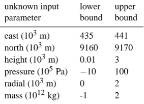
Table 1. Range limitations of the unknown input parameters used for the SA computation.
unknown input lower upper parameter bound bound
east (103m) 435 441 north (103m) 9160 9170 height (103m) 0.01 3 pressure (105Pa) −10 100 radial (103m) 0 2 mass (1012kg) -1 2
the measured changes in time. By anticipating a subsurface body which produces a given change in density and pressure between two measurement epochs, we can model both the location as well as the gravity on the surface. The observed changes in gravity and the three-dimensional displacements measured over a certain time period can be interpreted as the influence of this change in the source properties. Such a source can be modeled in volcanic areas as a magma cham-ber but also as another body, which is filled by a certain ma-terial and includes a specified pressure. Other possible expla-nations of such sources are voids that are filled with fluids, or bodies in which the gas pressure is increasing that would suggest highly explosive, dangerous volcanic activity.
The unknown parameters of the source (given by the east, north and height component as well as the pressure, radial and mass component) were determined by a non-linear in-version which is based on the Navier-Stokes equations, cou-pling elastic and gravitational effects. The inversion has been optimized by a GA approach, which maximizes the objec-tive function that is given as the 1/χ (comp.)2value. This is computed by taking all types of observations into account, Eq. (12). Initial samples, Tiede et al. (2004)1show that the location as well as the mass can be determined with only a small dispersion rate. However, the determination of the radial and pressure component of the source show large vari-ations which cover nearly the entire defined range of the un-known parameters. As a result, it follows that the determi-nation of the pressure and radial parameter is poorly con-strained, with high standard deviations of the mean values and signalling that these values could not be determined sig-nificantly.
Due to the fact that the sensitivity to the unknown parame-ters to the different types of is quite different, an investigation was made with the goal of stabilizing the inversion by the implementation of global SA results. The implementation is performed through a reweighting of the cofactor matriceQll
which is implied in the 1/χ (comp.)2value, Eq. (12). For that 1Tiede, C., Tiampo, K., Fern´andez, J., and Gerstenecker, C.: Ini-tial Inversion Results for Elastic Gravitational Modeling via Genetic Algorithms at Merapi Volcano, Indonesia, J. Volcanol. Geotherm. Res., submitted, 2004.
4.1 4.15 4.2 4.25 4.3 4.35 4.4 4.45 4.5 4.55 4.6 x 10⁵ 9.13
9.14 9.15 9.16 9.17 9.18 9.19x 10
6
east [m]
north [m]
4.38 4.39 4.4 9.166
9.167
Fig. 1. Distribution of those data locations used for the SA. Every observation point consists of gravity change as well as displace-ments in east, north and height direction.
purpose, the data set which was the basis of the work in Tiede et al. (2004)1 was used. The point distribution is given in Fig. 1. At each of the 20 observation points, gravity changes as well as displacements in the east, north and height compo-nent were determined. The topography is represented by the isolines. The limitation ranges of the unknown parameters for the quantitative SA are set according to initial results of the GA optimization (Tiede et al., 2004)1. The ranges were set large enough so that the computed results did not reach the limits of the defined ranges. These boundaries are sum-marized in Table 1.
2 Underlying physical model
The multimodal objective function is based on the general-ized Navier equations which couple elastic and gravitational effects in a homogeneous half space, given by Love (1911) and Rundle (1980)
0= ∇2u+ 1
1−2σ∇∇ ·u+ ρ0g
µ ∇(u·ez)
−ρ0
µ∇φ− ρ0g
µ ez∇ ·u+X (1)
∇2φ=4πρ0G∇ ·u+Y (2)
Rundle (1982) evaluates the equations that are satisfied by the displacement vector uand perturbation potential φ by obtaining a general solution at the heightz=0:
u=M
Z ∞
0
[x01(0)P0+y01(0)B0]kdk (3)
φ=M
Z ∞
0
ω10(0)J0(kr)kdk (4)
δg= −dφ
dz = −M
Z ∞
0
q01(0)J0(kr)kdk+4πρ0Guz (5)
withM=mass of the intrusion, x01(0), y01(0), ω01(0), q01(0) kernel functions, whose calculation is described in Rundle (1980), depend on the Fourier wave numberkand are given as a function of the characteristics of the medium’s lay-ers Fern´andez and Rundle (1994). P0,B0=vectors given in terms of Bessel functionJ0(kr)of the first kind of order zero andρ0= density of the layer.
For the purposes of this inversion Poisson’s ratioσ was chosen as 0.25 for an elastic medium and the Young’s mod-ulusEwas anticipated to be 30 GPa, according to Beaudu-cel et al. (2000). The mean density for this area is given as 2242 kg/m3, a value which was derived by preliminary grav-ity inversions in the area of interest.
3 Variance-based Sobol’ SA
Due to the non-linear property of the given inversion prob-lem, a global sensitivity analysis with the aim of apportioning the uncertainty in the output data due to the unknown input parameters was applied, Saltelli et al. (2000). Global SAs are based on the variation of all unknown input parameters at the same time, the computation over the full definition range of each unknown input parameter, and a form of probability density function (pdf) of each. In contrast, local SAs fix all unknowns and only vary one input parameter in a small range around the nominal value per time. A general global sen-sitivity concept, the variance-based SA is sampling-based, and therefore a Monte Carlo simulation is applied. In this work we applied Sobol’ as well as the Fourier amplitude SA, FAST, also belonging to this same kind of global SAs. The main advantage of these methods is that the analytic struc-ture of the model to be analyzed does not need to be known specifically. Schwieger (2004).
The main idea of these types of sensitivity analyses is based on the idea that one can determine the nature of the sensitivity through the varianceV and then evaluate how the input variance contributes to the output variance. By set-ting(X1, ..., Xk)as the vector of independent unknown input
parameters andY=f (X1, ..., Xk)as the output value, with
f as model function, an indicator for the importance of an inputXi can be set by evaluating the variance of the
out-putY V (Y|Xi). This is done by fixingXi to its true value
xi. V (Y|Xi) is called the conditional variance of Y with
Xi=xi. The true value of xi is not known, so instead of
V (Y|Xi)the expectation of the conditional variance, noted
asE[V (Y|Xi)]is studied, whereby it is built into all
possi-ble values ofxi. The variance ofY is given by
V (Y )=V (E[Y|Xi])+E[V (Y|Xi)]. (6)
The first addend is called the variance of the conditional ex-pectation and describes the importance ofXi on the variance
Y, which is equivalent to the sensitivity ofY toXi.
Normal-izing the sensitivity valueSias the ratio between the variance
of the expectation value and the variance of the output value leads to
Si =
V (E[Y|Xi])
V (Y ) (7)
and is called the first order sensitivity index, correlation ratio or importance measure and describes the main effect of the unknown parameterXion the output valueY. For an additive
model the summation over the ratios of the unknown param-eters results in 1, if interactions between the unknown input parameters exist, the entire decomposition of the objective function must be evaluated.
By propagating the variances of the unknown input param-eters through the model, which determines the influence of this unknown parameter on the model output variance, some of the variance-based techniques can deliver quantitative as well as model independent sensitivity results.
The variance-based Sobol’ sensitivity method explores the multidimensional space of the unknown input parametersX with a certain number of Monte Carlo samples. The sensitiv-ity indices, both first order and also the higher interactions between the unknown input parameters, related to Sobol’ (1993), are generated by a decomposition of the model func-tionf in ak-dimensional factor spacekinto summands of increasing dimensionality,
f (X1, ..., Xk)=f0+
k
X
i=1
fi(Xi)+
X
1≤i<j≤k
fij(Xi, Xj)
+...+f1,...,k(X1, ..., Xk) (8)
withX1, ..., Xk=unknown input parameters andf0=const. In all functions of the decomposition the integrals over any of its own variables are zero and they are orthogonal. All terms inf (X1, ..., Xk)can be evaluated by multidimensional
inte-grals.
Squaring and integrating Eq. (8) over k leads to the decomposition of the varianceV (X1, ..., Xk)of the output
valuef (X1, ..., Xk):
V (Y )= k
X
i=1 Vi+
X
1≤i<j≤k
Vij+...+V1,...,k (9)
with
Vi =V (E[Y|Xi]) (10)
Vij =V (E[Y|Xi, Xj] −E[Y|Xi] −E[Y|Xj])
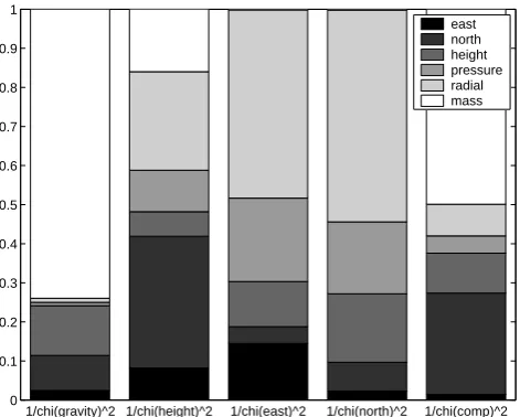
1/chi(gravity)^2 1/chi(height)^2 1/chi(east)^2 1/chi(north)^2 1/chi(comp)^2 0
0.1 0.2 0.3 0.4 0.5 0.6 0.7 0.8 0.9 1
east north height pressure radial mass
Fig. 2. Normalized Sobol’ first order indices for the five defined output parameters.
not correlated, the results can be obtained by
Vij =V (E[Y|Xi, Xj])−Vi −Vj (11)
The first order sensitivity indices are given bySi=Vi/V (Y ),
higher order indices bySi1,...,is =Vi1,...,is/V (Y ).
First order sensitivity indicesSimeasure the main effect of
each unknown parameterXi on the output and are
quantita-tive sensitivity results for addiquantita-tive models. The higher order indicesS(i1,...,is)describe the interaction effects between the
unknown input parametersXi1, ..., Xis on the output value.
These effects are not included in the individual effects of Xi1, ..., Xis.
The TSI of an unknown input parameterXi is defined as
the sum of all sensitivity indices, its main order effect as well as all the higher order effects in which this value appears. According to Saltelli et al. (2000) TSIs provide quantitative sensitivity analysis results for all kind of models independent of their model characteristics.
The SA, which is of an estimating nature, due to the lack of knowledge about the relation between input and output data as well as about the interactions between the unknown parameters, has been computed by the program Simlab, ver-sion 2.2, Saltelli et al. (2004). The general procedure to carry out the SA include the definition of the pdfs for the unknown input parameters, the generation of Monte Carlo samples for the unknown input parameters as well as the computation of the results of the physical underlying model using these samples, the analysis of the output variance, and a sensitivity analysis of the output variance in relation to the variation of the unknown input parameters, Schwieger (2004).
The unknown parameters east, north and height as well as pressure, radial and mass of the point source has been taken as input parameters for the quantitative, variance-based, global Sobol’ SA. The output is characterized by the 1/χ ()2 values, Eq. (12), including those for (gravity), (height), (east), (north) as well as (comp.) which is computed
1/chi(gravity)^2 1/chi(height)^2 1/chi(east)^2 1/chi(north)^2 1/chi(comp)^2 0
0.1 0.2 0.3 0.4 0.5 0.6 0.7 0.8 0.9 1
Fig. 3. Normalized Sobol’ Total Sensitivity Indices (TSI) for the five defined output parameters.
by taking all types of observations into account. Figure 1 shows an overview of the location configuration whereby at each of the 20 observation points, gravity changes, height, east and north displacements were measured. Theχ ()2 val-ues are computed by
χ ()2= v TQ
ll−1v
n−u (12)
withv as residuals between modeled and observed output values, specified by the type of observation(), Qll through a cofactor matrix. The given variances of each observation of()lie on its diagonal, anticipating uncorrelated data, with n−udegrees of freedom (nas number of observations,uas number of unknown parameters).
The pdf of the unknown values were assumed uniform due to the fact that it is not possible to specify any area or certain value ranges which are more likely than others within the given described bounds. The SA consists of 28 672 Monte Carlo samples. Figure 2 and Fig. 3, show the normalized Sobol’ first order indices and TSIs for the unknown input pa-rameters. The bar plots are given for each of the five defined output values 1/χ ()2separately.
By comparing the first order indices with the TSI’s, the results show clearly that only taking the first order indices into account would lead to large mistakes in the anticipa-tion of the influence of a certain unknown to the different kind of data. By computing the percentage of the first order effect compared to the corresponding TSI, only the sensi-tivity concerning the mass component for the output values 1/χ (gravity)2and 1/χ (north)2are influenced primarily by the first order indices. All other TSIs are driven primarily by interactions between the input parameters.
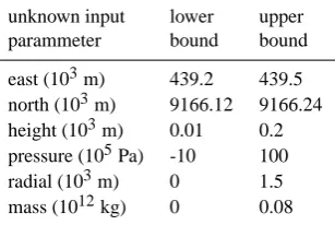
Table 2. Range limitations of the unknown input parameters used in the GA.
unknown input lower upper
parammeter bound bound
east (103m) 439.2 439.5 north (103m) 9166.12 9166.24 height (103m) 0.01 0.2 pressure (105Pa) -10 100 radial (103m) 0 1.5 mass (1012kg) 0 0.08
– 1/χ (gravity)2values are influenced in large part by the mass of the source. The three location parameters of the source have similar influences on this output value. 1/χ (gravity)2values are only few sensitive to changes in the pressure and radius of the unknown source.
– 1/χ (height)2values are, surprisingly, equally sensitive to the radial component as well to the north component of the source.
– 1/χ (east)2values are sensitive to changes in the radial component of the source and almost equally sensitive to changes in all other input parameters except the mass. The mass does not influence the output value at all.
– 1/χ (north)2values are most sensitive to changes in the radial component of the source. The mass has little to no influence and the east component has only a small influence. The other TSI’s are approximately the same size.
– 1/χ (comp.)2values are most sensitive to changes in the mass component as well as the north component. This summary of the different sensitivities concerning the unknown input parameters points out the great need of a joint inversion of both displacements and gravity changes.
4 Implementation of TSIs into GA
As mentioned in the introduction, initial results of a GA ap-proach, Tiede et al. (2004)1showed that the unknown param-eters pressure and radius of the source could not be deter-mined significantly without any additional information. The TSIs (caused by the unknown parameters) of the different 1/χ ()2values show that the sensibility of the observed dis-placements to changes in the radial component are much larger than the one of the gravity changes. Therefore, the TSI values governing the radial component TSI(r) of the un-known source has been taken as a reweighting factor in the cofactor matrix Qll(r)of the objective function 1/χ (comp.)2,
which is computed by taking all kind of measurements into
439.250 .3 .35
2 4 6
east [103 m]
number of samples
9166.2 .22 .24
0 2 4 6
north [103 m]
0 .05 .1
0 2 4
height [103 m]
0 50 100
0 2 4 6
pressure [105 Pa]
0.5 1
0 2 4 6 8 10
radial [103 m]
0 0.01 0.02
0 2 4 6
mass [1012 kg]
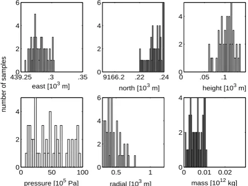
Fig. 4. Histograms for the unknown parameters computed by 50 GA samples without reweighting Qll.
account. The reweighted cofactor matrice Qll(r)is given by
Qll(r)=diag σgi ·
T SI (r) T SI (r)g
2
, σHi·
T SI (r) T SI (r)H
2
,
σEi·
T SI (r)
T SI (r)E
2
, σNi·
T SI (r)
T SI (r)N
2!
(13) T SI (r)=T SI (r)g+T SI (r)H +T SI (r)E+T SI (r)N
with i=1...20, σg, σH, σE and σN=variance of gravity
change, change in height, east and north component of the i-th observation point.
Fifty samples of a GA approach, explained in detail in Tiampo et al. (2000), have been computed with the im-plemented reweighted Qll(r) matrix and are compared to
the original samples which were carried out without any reweighting. The population size is given by 100. 1000 is chosen as the maximum number of generations, the limita-tion bounds for the unknown parameters are set equal, Ta-ble 2.
The results of the computation are shown in Fig. 4 for the GA optimization without reweighting and in Fig. 5 for the GA optimization with reweighting Qll(r) of the TSIs for
the radial component of the unknown source. Table 3 lists the ranges of the unknown parameters for these two different computations. It can be seen that all ranges were decreased by the reweighted Qll(r).
Comparing theχ (comp.)2values of the best two models shows that the model with the reweightedQll(r)matrix leads
toχ (comp.)2=115.847, whereby the best model determined by the normal GA leads toχ (comp.)2=115.642. The small change for the worse of the reweighted result is explained by examination of the standard deviations of the output val-ues whose weights are now changed according to the Qll(r)
Table 3. Ranges of unknown parameters determined by 50 sample of GA without and with reweighting Qll(r).
unknown range without range with parameter reweighting Qll reweighting Qll(r)
east (103m) 0.059 0.048
north (103m) 0.041 0.019 height (103m) 0.079 0.077 pressure (105Pa) 94.548 89.402 radial (103m) 0.752 0.462 mass (1012kg) 0.017208 0.010536
5 Conclusions
The paper reviews the application of Sobol’ variance-based SA, a quantitative global method for the determination of the TSI’s of the unknown input parameters for each kind of ob-served output value.
The application of the Sobol’ sensitivity analysis shows different sensitivities for the different 1/χ ()2 output val-ues. In particular, the sensitivity concerning the mass, radial and pressure components for the 1/χ (gravity)2 compared to the sensitivity against those values of the 1/χ (height)2, 1/χ (east)2 and 1/χ (north)2 are very different. These dif-ferent sensitivities demonstrate that there is a great need to invert gravity changes and displacement data in a common approach for the determination of an elastic-gravitational source.
Furthermore, if the different types of observation data show different sensitivities against the unknown input pa-rameters, this information can be used to determine spe-cial unknown input parameters in more detail. By enlarging the weights of those observations which are most sensitive against differences of a certain unknown input parameter, this special unknown can be determined more accurately.
In this example, the reweighting approach results in a more homogeneous optimization. The sum of all residuals concerning gravity and displacement observations constructs the objective function to be minimized. By introducing the reweighting approach, the influence of the dominant sensi-tivity relating to the mass component of the gravity observa-tions has been reduced, and the influence of the sensitivity concerning the radial component could be increased by the increase in the weights of the displacements.
The results of this approach show that it is possible to en-large the accuracy of the determined radial component by the implementation of the reweighting factors. Although the fitness of the best chosen model is decreasing by a small amount, the benefits of the implementation are obvious.
The introduced implementation of the sensitivity analysis into an optimization might be applied in a many areas of in-terest. If the objective function is computed by the sum of different types of residuals (in this approach observed grav-ity changes, height, east and north displacements) and these
439.250 .3 .35
2 4 6
east [103 m]
9166.2 .22 .24
0 2 4 6
north [103 m]
number of samples
0 .05 .1
0 2 4
height [103 m]
0 50 100
0 2 4
pressure [105 Pa]
0.5 1
0 2 4 6
radial [103 m]
0 0.01 0.02
0 2 4
mass [1012 kg]
Fig. 5. Histograms for the unknown parameters computed by 50 GA samples with reweighting Qll(r)by the TSIs.
observations have different sensitivities to the unknown input parameters, the information of the TSIs can be used to stabi-lize the optimization results. In that case, the reweighting according to the TSIs must be incorporated into the cofactor matrix Qll(r) in order to change the weights of the various
types of output values according to their sensitivity.
Acknowledgements. This research is supported by a scholarship financed by Deutscher Akademischer Austauschdienst. Data resulting from a project supported by the Deutsche Forschungs-gemeinschaft under GE381/12. CT would like to acknowledge the Department of Earth Science of Western University, London Ontario for their great support as well as their hospitality during the completion of this work. The research by KFT has been funded by a UWO ADF grant. The research by JF has been funded under MCyT project REN2002-03450.
Edited by: G. Z¨oller
Reviewed by: V. Schwieger and two referees
References
Beauducel, F., Cornet, F., Suhanto, E., Duquesnoy, T., and Kasser, M.: Constraints on Magma Flux from Displacements Data at Merapi Volcano, Java, Indonesia, J. Geophys. Res., 105, 8193– 8204, 2000.
Fern´andez, J. and Rundle, J.: Gravity Changes and Deformation due to a Magmatic Intrusion in a Two-Layered Crustel Model, J. Geophys. Res., 99, 2737–2746, 1994.
Love, A.: Some Problems in geodynamics, Cambridge University Press, New York, 1911.
Peterson, R. and Dean, K.: Sensitivity of Puff: a Volcanic Ash Parti-cle Tracking Model, Tech. rep., University of Alaska, Fairbanks, 2003.
Rundle, J.: Static Elastic-Gravitational Deformation of a Layered Half-Space by Point Couple Sources, J. Geophys. Res., 85, 5355–5363, 1980.
Rundle, J.: Deformation, Gravity, and Potential Changes due to Vol-canic Loading of the Crust, J. Geophys. Res., 88, 647–652, 1982. Saltelli, A., Chan, K., and Scott, E. (Eds.): Sensitivity Analysis,
John Wiley and Sons, LTD, 2000.
Saltelli, A., Tarantola, S., Campolongo, F., and Ratto, M.: Sensitiv-ity Analysis in Practice, John Wiley & Sons, Ltd., 2004. Schmid, M., Lorke, A., W¨uest, A., Halbwachs, M., and Tanyileke,
G.: Development and sensitivity analysis of a model for assess-ing stratification and safety of Lake Nyos durassess-ing artificial de-gassing, Ocean Dynamics, 53, 288–301, 2003.
Schwieger, V.: Variance-based sensitivity Analysis for Model eval-uation in engineering Survey, INGEO 2004 and FIG Regional Central and Eastern European Conference on Engineering Sur-veying Bratislava, Slovakia, 11–13 November, 2004.
Sobol’, I.: Sensitivity Analysis for non Linear Mathematical Mod-els, Math. Model. Comput. Exp., 1, 407–414, 1993.
Tiampo, K., Rundle, J., Fern´andez, J., and Langbein, J.: Spherical and Ellipsoidal Volcanic Sources at Long Valley Caldera, Cali-fornia, Using a Genetic Algorithm Inversion Technique, J. Vol-canol. Geotherm. Res., 102, 189–206, 2000.