Macro-roughness model of bedrock–alluvial river morphodynamics

www.earth-surf-dynam.net/3/113/2015/ doi:10.5194/esurf-3-113-2015

© Author(s) 2015. CC Attribution 3.0 License.

Macro-roughness model of bedrock–alluvial

river morphodynamics

L. Zhang1, G. Parker2, C. P. Stark3, T. Inoue4, E. Viparelli5, X. Fu1, and N. Izumi6 1_{State Key Laboratory of Hydroscience and Engineering, Tsinghua University, Beijing, China} 2_{Department of Civil & Environmental Engineering and Department of Geology, Hydrosystems Laboratory,}

University of Illinois, Urbana, IL, USA

3_{Lamont-Doherty Earth Observatory, Columbia University, Palisades, NY, USA} 4_{Civil Engineering Research Institute for Cold Regions, Hiragishi Sapporo, Japan} 5_{Dept. of Civil & Environmental Engineering, University of South Carolina, Columbia, SC, USA}

6_{Faculty of Engineering, Hokkaido University, Sapporo, Japan}

Correspondence to: L. Zhang ([email protected])

Received: 14 April 2014 – Published in Earth Surf. Dynam. Discuss.: 27 May 2014 Revised: 6 January 2015 – Accepted: 6 January 2015 – Published: 11 February 2015

1 Introduction

The pace of river-dominated landscape evolution is set by the rate of downcutting into bedrock across the channel network. The coupled process of river incision and hillslope response is both self-promoting and self-limiting (Gilbert, 1877). Al-though there are multiple processes that can lead to erosion into bedrock, we here focus on incision driven by abrasion of a bedrock surface as moving particles collide with it. Low rates of incision entail some sediment supply from upstream hillslopes, which provides a modicum of abrasive material in river flows that further facilitates bedrock channel erosion. Faster downcutting leads to higher rates of hillslope sedi-ment supply, boosting the concentration of erosion “tools” and bedrock wear rates, but also leading to greater cover of the bedrock bed with sediment (Sklar and Dietrich, 2001, 2004, 2006; Turowski et al., 2007; Lamb et al., 2008; Tur-owski, 2009). Too much sediment supply leads to choking of the channels by alluvial cover and the retardation of further channel erosion (e.g., Stark et al., 2009). This competition between incision and sedimentation leads long-term eroding channels to typically take a mixed bedrock–alluvial form in which the pattern and depth of sediment cover fluctuate over time in apposition to the pattern of bedrock wear.

Theoretical approaches to treating the erosion of bedrock rivers have shifted over recent decades (see Turowski, 2012, for a recent review). The pioneering work of Howard and Kerby (1983) focused on bedrock channels with little sed-iment cover; it led to the detachment-limited model of Howard et al. (1994), in which channel erosion is treated as a power function of river slope and characteristic discharge, and the “stream-law” approach, in which the power-law scaling of channel slope with upstream area underpins the way in which landscapes are thought to evolve (Whip-ple and Tucker, 1999; Whip(Whip-ple, 2004; Howard, 1971, fore-shadows this approach). At the other extreme, sediment flux came into play in the transport-limited treatment of mass re-moval from channels of, for example, Smith and Brether-ton (1972), in which no bedrock is present in the channel and where the divergence of sediment flux determines the rate of lowering. Whipple and Tucker (2002) blended these approaches, and imagined a transition from detachment lim-itation upstream to transport-limited behavior downstream. They also discussed, in the context of the stream-power-law approach, the idea emerging at that time (Sklar and Di-etrich, 1998) of a “parabolic” form of the rate of bedrock wear as a function of sediment flux normalized by transport capacity. Laboratory experiments conducted by Sklar and Dietrich (2001) corroborated this idea, and they led to the first true sediment flux-dependent model of channel erosion of Sklar and Dietrich (2004, 2006). This saltation–abrasion model was subsequently extended by Lamb et al. (2008) and Chatanantavet and Parker (2009). It was explored experi-mentally by Chatanantavet and Parker (2008) and Chatanan-tavet et al. (2013); evaluated in a field context by Johnson

et al. (2009), Chatanantavet and Parker (2009), Hobley et al. (2011) and Turowski et al. (2013); adapted to treat al-luvial intermittency by Lague (2010); and given a stochastic treatment by Turowski et al. (2007), Turowski (2009) and Lague (2010), the latter of whom introduced several new el-ements. Howard (1998) presents an alternative formulation for incision that relates bedrock wear to the thickness of al-luvial cover rather than sediment supply, in a form that can be thought to be a predecessor of the present work.

At the heart of their saltation–abrasion model lies the idea of a cover factorpcorresponding to the areal fraction of the bedrock bed that is covered by alluvium (Sklar and Diet-rich, 2004). This bedrock bed is imagined as a flat surface on which sediment intermittently accumulates and degrades during bedload transport over it. The fraction of sediment cover is assumed to be a linear function of bedload transport relative to capacity. Bedrock wear takes place when bedload clasts strike the exposed bedrock. In the simplest form of the saltation–abrasion model, the subsequent rate of bedrock wear is treated as a linear function of the impact flux and in-ferred to be proportional to the bedload flux, which leads to the parabolic shape of the cover-limited abrasion curve.

The saltation–abrasion model is considerably more so-phisticated and flexible (Sklar and Dietrich, 2004, 2006) than this sketch explanation can encompass. It does, however, have three major restrictions. First, it is formulated in terms of sediment supply rather than local sediment transport. The model is thus unable to capture the interaction between pro-cesses that drive evolution of an alluvial bed and those that drive the evolution of an incising of bedrock–alluvial bed. Second, for related reasons, it cannot account for bedrock to-pography significant enough to affect the pattern of sediment storage and rock exposure. Such a topography is illustrated in Fig. 1 for the Shimanto River, Japan. Third, it is designed for quasi-steady conditions, and thus cannot account for the effects of cyclic variation in sediment supply on channel de-velopment downstream of the point of sediment supply.

a

b

Figure 1.Views of the Shimanto River, a mixed alluvial–bedrock river in Shikoku, Japan. (a) Upstream view at low stage. (b) Macro-scopic roughness of the bed and alluvial patches. Channel width is about 100 m.

presented here. The notation used in this paper is defined in Table A1.

2 Capacity-based Saltation-Abrasion (CSA) geomorphic incision law and its implications for channel evolution: upstream-migrating waves of incision

2.1 CSA geomorphic incision law

Sklar and Dietrich (2004, 2006) present the following model, referred to here as the Capacity-based Saltation-Abrasion (CSA) model, for bedrock incision in mixed bedrock– alluvial rivers transporting gravel. DefiningEas the vertical rate of erosion into bedrock,qaas the volume gravel transport

rate per unit width (specified in their model solely in terms of a supply, or feed rateqaf) andqacas the capacity volume

gravel transport per unit width such thatqa < qac,

E=βqa

1− qa qac

, (1a)

whereβ is an abrasion coefficient with dimension L−1. By introducing a cover factor parameterp, this equation can be rewritten as

E=βqacp(1−p). (1b)

This cover factorp is defined (Sklar and Dietrich, 2006) as the areal fraction of bedrock surface covered with alluvium and is given by

p=

  

 

qa

qac . . . 0≤ qa qac≤1

1. . . qa

qac >1,

(2)

where this fraction is calculated by averaging over a win-dow larger than a characteristic macroscale of bedrock ele-vation variation. We refer to this formulation for cover factor pas “capacity based” because Eq. (2) dictates thatpis deter-mined in terms of the ratio of sediment supply to its capacity value in the CSA model.

In the above formulation, it is assumed that the gravel transport rateqaover a bedrock surface can be estimated by

simply multiplying the capacity rateqac by the areal cover

fractionp. While this is the simplest first-order assumption, it should be recognized that the roughness of the bedrock it-self can change the flow resistance, leading to a relationship that is more complex than Eq. (1b) (Inoue et al., 2014; John-son, 2014).

Before introducing the relation of Sklar and Diet-rich (2006) for abrasion coefficientβ, it is of value to pro-vide an interpretation for this parameter not originally given by Sklar and Dietrich (2004, 2006), but which plays a use-ful role in the analysis below. The abrasion coefficient has a physical interpretation in terms of Sternberg’s law (Stern-berg, 1875) for downstream diminution of grain size (Parker, 1991, 2008; Chatanantavet et al., 2010). The analysis leading to this interpretation is given in Appendix A; salient results are summarized here. Consider a clast of material that is of identical rock type to the bedrock being abraded. Sternberg’s law is

D=Due−αdx, (3)

whereDis gravel clast size,Duis the upstream value ofD,

xis downstream distance andαdis a diminution coefficient.

If all diminution results from abrasion,αdis related toβby

αd=

β

3. (4a)

In the case of constantβ, and therefore constantαd, the

dis-tanceLhalffor such a clast to halve in size is given by

Lhalf=

ln(2) αd

This interpretation of abrasion coefficient β in terms of diminution coefficientαd allows for comparison of the

ex-perimental results of Sklar and Dietrich (2001) with values ofαdpreviously obtained from abrasion mills (Parker, 2008:

see Fig. 3-41 therein; Kodama, 1994).

The relations of Sklar and Dietrich (2004, 2006) to com-puteβandqaccan be cast in the following form:

β=0.08ρgRgY kσ_t2

_τ∗

τ∗

c

−1

−1/2" 1−τ

∗

R_f2

#3/2

, (5a)

Rf=

vf

√

RgD, (5b)

qac=αa p

RgD D τ∗−τ_c∗na_{. (5c)}

In the above relations, D corresponds to the characteristic size of the gravel clasts that are effective in abrading the bedrock; ρgis the material density of the grains; R is their

submerged specific gravity (∼1.65 for quartz);gis gravita-tional acceleration,τ∗ is the dimensionless Shields number of the flow;τ_c∗is the threshold Shields number for the onset of significant bedload transport; αa andna denote,

respec-tively, a relation-specific dimensionless coefficient and an ex-ponent;vfis the fall (settling) velocity corresponding to grain

sizeD,Y is the bedrock modulus of elasticity;σtis the rock

tensile strength; and kis a dimensionless coefficient of the order of 10−6. (In the above two relations and the text, sev-eral misprints in Sklar and Dietrich (2004, 2006) have been corrected on the advice of the authors.) Equation (5c) corre-sponds to the bedload transport relation of Fernandez Luque and van Beek (1976) whenαa=5.7 andna=1.5; Sklar and

Dietrich (2004, 2006) used this relation with the assumed valueτ_c∗=0.03.

The relations above define a 0-D formulation. It must be augmented with other parameters and relations, including channel width, relations for hydraulics, quantification of flow discharge or flow duration curve, etc., to allow application at the river reach scale.

It is useful to cast Eq. (5a) in the form

β=βref

τ∗ τ∗

c −1

−1/2 1−τ∗

R2_f

3/2

_τ∗

ref τ∗

c −1

−1/2 1−τ

∗

ref R2_f

3/2, (5d)

whereβrefis a reference value ofβ, either computed from

known values of the parametersY,k,σt,Rf, etc., or estimated

indirectly.

2.2 Embedding of CSA into a model of bedrock surface evolution

A relation for the evolution of bedrock surface elevationηb

is obtained by substituting the CSA geomorphic law for in-cision of Eq. (1b) into a simplified 1-D mass conservation

equation for bedrock material subjected to piston-style rock uplift or base level fall (Sklar and Dietrich, 2006):

∂ηb

∂t =υ−I E. (6a)

Heret denotes time,υ denotes the relative vertical veloc-ity between the rock underlying the channel (which is as-sumed to undergo no deformation) and the point at which base level is maintained, andI denotes a flood intermittency factor to account for the fact that only relatively rare flow events are likely to drive incision (Chatanantavet and Parker, 2009). Also,Iis assumed to be a prescribed constant; a more generalized formulation for flow hydrograph is given in Sklar and Dietrich (2006) and DiBiase and Whipple (2011). In in-terpreting Eq. (6a), it should be noted thatυdenotes a rock uplift rate (in the sense of England and Molnar, 1990) for the case of constant base level, or equivalently a rate of base level fall for rock undergoing neither uplift nor subsidence. Below we use the term “rock uplift” as shorthand for the rel-ative vertical velocity between the rock and the point of base level maintenance. Substituting Eq. (1b) into Eq. (6a) yields (Sklar and Dietrich, 2006)

∂ηb

∂t =υ−Iβqacp(1−p). (6b)

2.3 Character of the CSA model: upstream waves of incision

The MRSAA model (introduced below) has several new fea-tures as compared to CSA. These are best illustrated by first characterizing the mathematical nature of CSA in the context of Eq. (6). Let

Sb= −

∂ηb

∂x (7)

denote the streamwise bedrock-surface slope. Reducing Eq. (6b) with Eq. (7) the CSA model of Eq. (1) reveals it-self as a nonlinear kinematic wave equation with a source term:

∂ηb

∂t −cb ∂ηb

∂x =υ, (8a)

cb=

Iβqacp(1−p)

Sb

. (8b)

Here cb denotes the wave speed associated with bedrock

incision. The form of Eq. (8a) dictates that disturbances in bedrock elevation always move upstream. We will see later that these disturbances can take the form of upstream-migrating knickpoints (e.g., Chatanantavet and Parker, 2009).

assumption allows for simplification. LetQdenote water dis-charge during (morphodynamically active) flood flow taking place with intermittencyI, and letH denote flood depth and g denote acceleration due to gravity. Momentum and mass balance take the forms

τ =ρgH Sb, (9a)

Q=U BH, (9b)

whereτ is boundary shear stress at flood flow,Uis the cor-responding mean flow speed, B is channel width andρ is water density. The dimensionless Shields numberτ∗and di-mensionless Chézy resistance coefficientCzare defined as

τ∗= τ

ρRgD, (10a)

Cz=√U

τ/ρ. (10b)

As shown in Parker (2004) and Chatanantavet and Parker (2009), reducing Eqs. (7), (9) and (10) yields the fol-lowing relations forHandτ∗:

H=

Q2 Cz2_gB2_S

b 1/3

, (11a)

τ∗=

Q2 Cz2_gB2

1/3_S2/3 b

RD. (11b)

A comparison of Eqs. (2), (5c) and (11b) indicates that even for constant values of other parameters, the functional forms for qacand thuspare such thatcbis in general a nonlinear

function ofSb= −∂ηb/∂x.

2.4 Limitations of the CSA model

The CSA model (Sklar and Dietrich, 2004, 2006) was a ma-jor advance in the analysis of bedrock incision due to abra-sion because it (a) accounts for the effect of alluvial cover and tool availability on the incision rate through the term p(1−p) in Eq. (1b) and (b) provides a physical basis for incision due to abrasion as gravel clasts collide with the bedrock surface. The CSA model been used, modified, adapted and extended by a number of researchers (Crosby et al., 2007; Lamb et al., 2008; Chatanantavet and Parker, 2009; Turowski, 2009; Lague, 2010).

The model does, however, have a significant limitation in that it specifically does not include either alluvial mor-phodynamics or the mormor-phodynamics of transitions between bedrock and alluvial zones. Here we study this limitation, and how to overcome it, in terms of the highly simplified configuration of a reach (HSR, highly simplified reach) with constant width; fixed, non-erodible banks; constant water discharge; and sediment input only from the upstream end. For simplicity, we also neglect abrasion of the gravel itself, so that grain size D is a specified constant. (This condi-tion, while introduced arbitrarily here, can be physically in-terpreted in terms of clasts that are much more resistant to

abrasion than the bedrock.) The means to relax these con-straints is available (e.g., Chatanantavet et al., 2010; DiBiase and Whipple, 2011), and indeed many of them have been implemented in the SSTRIM model of Lague (2010). Such a relaxation, however, obscures the first-order physics under-lying the rich patterns of interaction between completely and partially alluviated conditions illustrated herein.

In the CSA model, the bedload transport rateqais

speci-fied as a “supply”. That is, the bedload transport rate is con-strained so that it cannot change in the downstream direc-tion, and is always equal to the bedload feed rate (supply) qafat the upstream end. When the feed rateqafincreases,qa

must increase simultaneously everywhere. That is, a change in bedload supply is felt instantaneously throughout the en-tire reach, regardless of its length.

We illustrate this behavior in Fig. 2. The reach has length L. The gravel feed rate at x=0 follows a cyclic “sedimentograph” (in analogy to a hydrograph) with period T=Th+Tl, in which the sediment feed rate has a constant

high feed rateqafhfor timeTh, and a subsequent constant low

feed rateqafl for time Tl. According to the CSA model, at

x=Lcorresponding to the downstream end of the reach, the temporal variation in bedload transport rate must precisely reflect the feed rate. That is, the model was not designed to route sediment in the downstream direction.

In a more realistic model, the effect of a change in bedload feed rateqaf would gradually diffuse and propagate

down-stream, so that the bedload transport rate at the downstream end of the reach would show more gradual temporal vari-ation. This effect is illustrated in Fig. 2. This same diffu-sion and propagation can be expected in the cover fractionp, which in general should vary in bothx andt. The change in cover fraction in turn should affect the incision rate as quanti-fied in Eq. (1a). To capture this effect, however, Eq. (1b) must be coupled with an alluvial formulation that routes sediment downstream over the bedrock.

A second limitation concerns alluviation of the bedrock surface. Consider a wave of sediment moving over this sur-face, as shown in Fig. 3. We characterize the vertical scale of the geometric roughness of the bedrock surface (as seen in Fig. 1) in terms of a vertical macro-roughnessLmr. For

sim-plicity, we assume that the bottom of the bedrock relief has a specific elevationηb, an assumption that will be relaxed later

in favor of a probabilistic formulation. The alluvial thickness above this basal elevationηa represents an average value of

local bed elevation over an appropriately defined window. It can be seen in Fig. 3 that the surface undergoes both partial (ηa< Lmr) and then complete (ηa≥Lmr) alluviation, only to

be excavated later as the wave passes through. Bed elevationηis given as

η=ηb+ηa. (12)

0 0 feed sedimentograph

qafl qafh

upstream downstream

q

t

t

q

unmodified feed

advected and diffused

T_h Th+Tl Th Th+Tl

0

x

exit sedimentograph

Figure 2.Schematic diagram illustrating downstream modification of a sedimentograph. At the upstream feed point (x=0, left panel), the bedload transport rateqatakes the high feed valueqafhfor timeThand the low feed valueqafltimeTl, for a total cycle time ofT=Th+Tl. At the downstream end (x=L, right panel), the discontinuous brown line represents the unaltered sedimentograph at the downstream end of the reach, assumed to have propagated instantaneously from the supply point, while the smoother red line represents the sedimentograph as modified by advective–diffusive effects.







L

Figure 3.Schematic diagram illustrating the propagation of a wave of sediment over bedrock (orange line shifting to dashed orange line over time). Here ηb denotes the elevation of the bottom of the bedrock relief (black line), Lmr denotes the bedrock macro-roughness thickness (dashed black line),ηa denotes the thickness of the alluvial cover (which may be less than or greater thanLmr) andη=ηb+ηadenotes the elevation of the top of the alluvium.

corresponding to the thicknessηa. The CSA model does not

describe the variation in bed elevationη when the bed un-dergoes transitions between partial and complete alluviation; it simply infers that incision is shut down by the complete alluvial cover.

The goal of this paper is the development and implemen-tation of a model that overcomes these limiimplemen-tations by (a) cap-turing the spatiotemporal coevolution of the sediment trans-port rate, alluvial cover thickness and bedrock incision rate, and (b) explicitly enabling spatiotemporally evolving transi-tions between bedrock–alluvial morphodynamics and purely alluvial morphodynamics. The form of the model presented here is simplified in terms of the HSR outlined above, includ-ing a constant-width channel and a sinclud-ingle sediment source upstream.

3 Macro-Roughness-based

Saltation-Abrasion-Alluviation (MRSAA) formulation and its implications for channel evolution

3.1 Formulation for alluvial sediment conservation and cover factor

The geomorphic incision law of the MRSAA model is iden-tical to that of CSA, i.e., Eq. (1b). The essential differences are contained in (a) a formulation for the cover factorpthat differs from Eq. (2) and (b) the inclusion of alluvial morpho-dynamics in a way that tracks the spatiotemporal evolution of the bedload transport rate, and allows for smooth spatiotem-poral transitions between the bedrock–alluvial state and the purely alluvial state.

The specific case we consider here is one for which (a) the bedrock surface is rough in a hydraulic sense (as opposed to a hydraulically smooth or transitional surface; see Schlichting, 1979), and (b) the characteristic vertical scale of bedrock el-evation fluctuation about a mean value based on an appropri-ately defined window, here denoted as the macro-roughness Lmr of the bedrock, is large compared to the characteristic

size of the clasts constituting the alluvium. We use the term “macro-roughness” so as to clearly distinguish it from hy-draulic roughness, which is specifically defined in terms the logarithmic velocity profile. Inoue et al. (2014) introduced the terms “clast-rough” and “clast-smooth”, the former refer-ring to a bedrock surface roughness that is large compared to the characteristic size of the alluvium, and the latter referring to a bedrock surface macro-roughness that is small compared to the size of the alluvium. Here we specifically consider the clast-rough case.

p0

~ p~ p1

~

z'0

z'1

z

z'

_b Lmr

0 1

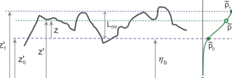
Figure 4.Illustration of the statistical structure or local hypsometry of the bedrock surface topography (dark-grey line). Herez0denotes an elevation above some arbitrary datum (dark-red line) deep in the bedrock andp(ze

0_{)is the probability (green line, marker) that a point}

at elevationz0is in water or alluvium rather than bedrock, i.e., above the local bedrock surface. The effective “bottom” of the bedrock re-lief is located at elevationz₀0=ηb, wherepetakes an appropriately

selected low valuepe1(e.g., 0.05); the effective “top” of the bedrock

relief is located at elevationz0₁, wherepetakes an appropriately

se-lected high valuepe1(e.g., 0.95); and the macro-roughnessLmris

given asz0₁−z0₀. The coordinatez=z0−z0₀is referenced to the ef-fective “bottom” of the bedrock relief.

to Struiksma (1999), and further progress has been made by Parker et al. (2009, 2013), Izumi and Yokokawa (2011), Izumi et al. (2012), Tanaka and Izumi (2013) and Zhang et al. (2013). These models are expressed in continuous form; Lague (2010) presents a discrete version based on a series of reaches of finite length that allows for generalization to a continuous form.

None of the above models is specifically designed to han-dle the clast-rough case, in particular that shown in Fig. 1, where the elevation of the bedrock roughness has a random element. Here we handle the clast-rough case by first charac-terizing the statistical nature of the bedrock surface alone. As noted in Fig. 4,z0denotes elevation above an arbitrary datum deep in the bedrock, andp(z_e 0)denotes the probability that a point located at elevation z0 is located in alluvium or water rather than bedrock. Conversely, 1−

e

pdenotes the probabil-ity that a point at elevationz0is in bedrock (rather than water or alluvium above). As seen on the right-hand side of the figure,_ep(z0)→0 asz0→ −∞(pure bedrock) and_ep(z0)→1 asz0→ +∞. This statistical structure function (a hypsomet-ric curve for local bedrock topography) which we use here to characterize bedrock elevation fluctuations is analogous to that used in Parker et al. (2000) for alluvial beds. It should be noted that “−∞” is shorthand for “far below the bedrock surface” and “+∞” is shorthand for “far above the bedrock surface”. It should also be emphasized that the tilde in the parameter_epindicates it is not a cover factor, but rather a sta-tistical parameter referring to the bedrock relief itself.

In such a statistical formulation, bedrock relief has neither a precise “bottom” nor a precise “top”. Rather, the “bottom” and “top” of the bedrock topography, as well as the macro-roughnessLmr, are here defined in a statistical sense. This

a

_b

z' z z

 _Lmr

Figure 5.Schematic diagram for derivation of the Exner equation of sediment continuity over a bedrock surface (dark-grey line). As in Figs. (3) and (4),zis the elevation above the effective “bottom” of the bedrock relief,Lmris macro-roughness height,ηbis elevation at base of the bedrock andηais the thickness of alluvium (yellow fill). The diagram shows alluvium–water interfaces (blue line) that are at spatially constant elevations. This is for illustrative purposes only; the interfaces should instead be those that result from averag-ing over an appropriate spatial window, i.e., alluvial fill levels are expected to vary from one pocket in the bedrock relief to another.

can be done using moments or exceedance probabilities; here we use the latter.

Let p_e0 denote some low reference value of pe (e.g., p_e0=0.05, or deep into the bedrock relief) and

e

p1 denote a corresponding high reference value of pe (e.g., p_e1=1−pe0=0.95, or near the upper portion of the bedrock relief), andz0₀andz0₁denote the corresponding bed elevations. An effective “base” of the bedrock relief can be set atz0₀, a macro-roughness heightLmrdefined as

Lmr=z01−z

0

0 (13)

and an effective “top” of the bedrock specified asz0₀+Lmr.

The clast-rough condition considered here satisfies the con-straint thatLmr/D1.

The problem can now be rephrased in terms of a vertical coordinatezwith its origin located at the effective bottom of the bedrock topography:

z=z0−z0₀. (14)

As noted in Fig. 4, the statistical variable_ep(z)with shifted coordinateznow has the following properties:

e

p(z=0)=

e

p0, ep (z=Lmr)=pe1. (15)

Here we define the thickness of the alluvial coverηa as the

elevation difference between the locally averaged top of the alluvium and the elevationz=0. The cover fractionp asso-ciated with any alluvial thicknessηa relative to the

macro-roughness heightLmris then given as

p (ηa/Lmr)=ep (z=ηa) . (16)

3.2 Exner equation of alluvial sediment conservation over a bedrock surface

unit area between elevationszandz+1zis (1−λ)p(z) 1z_e , and the corresponding volume bedload transport rate per unit width qa is estimated as p qac, where again, according to

Eq. (16),p=

e

p(ηa).

For the case of sediment of constant density, the Exner equation for mass balance of alluvial sediment can be ex-pressed as

(1−λ)∂ ∂t

ηa

Z

0 e

pdz= −I∂pqac

∂x , (17)

where the factorI accounts for the fact that morphodynam-ics are active only during floods. Reducing Eq. (17) using Leibniz’s rule,

(1−λ)p∂ηa

∂t = −I

∂pqac

∂x . (18)

The above formulation for the conservation of alluvial sedi-ment over a bedrock surface differs in one essential way from the earlier forms due to Struiksma (1999), Parker et al. (2009, 2013), Izumi and Yokokawa (2011), Izumi et al. (2012), Tanaka and Izumi (2013) and Zhang et al. (2013). Specifi-cally, in Eq. (18), the cover fractionpis present on the left-hand side of the equation as well as the right-left-hand side. It is shown below that this feature dictates a strong nonlinearity in the speed of propagation of alluvial waves over a bedrock surface, such that wave speed increases with decreasing wave amplitude. This feature is specifically captured by means of Leibniz’s rule, as implemented between Eqs. (17) and (18).

The combination of Eqs. (6b) and (18) delineates a formu-lation encompassing both mixed bedrock–alluvial rivers and alluvial rivers.

3.3 Closure model for cover relation

In the present formulation, the cover fractionpis free to vary in both x and t, i.e., p=p(x, t ). In order to complete the problem, however, it is necessary to specify a closure model for p. We characterize the local variation in bedrock eleva-tion in terms of the macro-roughness, i.e., the vertical length scale Lmr of Fig. 4. Here we seek a formulation that

aver-ages over a window capturing a statistically relevant sample of this local variation. In general, we assume a cover relation that characterizes to what extent the alluvial cover “drowns” the bedrock roughness elements. More specifically, we as-sume the form

p=f (χ ), (19a)

χ= ηa

Lmr

≥0, (19b)

f (χ=0)=

e

p0, (19c)

f (χ=1)=

e

p1. (19d)

The precise details of the relation can be expected to vary from case to case, but the overall characteristics that we hy-pothesize are illustrated in Fig. 6a–c. It is seen therein thatp

takes the residual valuep=

e

p0(e.g., 0.05) atχ=0, increases

monotonically top=

e

p1(e.g., 0.95) atχ=1, and then takes

the asymptotic valuep→1 asχ becomes sufficiently large. The first of these conditions corresponds to a bedrock sur-face that is bare of alluvium except in deep pockets of the macro-roughness elements, the second to a bedrock surface that is nearly completely alluviated but with some parts of the macro-roughness elements exposed, and the third to a bedrock surface that is deeply alluviated.

Note that the cover relation of Fig. 6 and Eq. (19) is based on the macro-roughness height scaleLmr rather than

the transport capacityqac of Eq. (2). This is the motivation

for referring to the new model presented here as the Macro-Roughness-based Saltation-Abrasion-Alluviation (MRSAA) model.

In applying the MRSAA model to general cases, it is use-ful to delineate the simplest functional form for the closure relation for cover fraction that satisfies the constraints of Eq. (19) and Fig. 6. This relation is the piecewise-linear form

p=f (χ )=

 

 e

p0+(pe1−pe0) χ . . .0≤χ≤

1−_ep0

e p₁−

e p₀

1 . . . χ > 1−ep0

e p1−pe0

(20a)

or rephrasing to emphasize the dependence ofpon the thick-ness of alluvial coverηa,

p=f (ηa/Lmr)=  

 e

p0+(ep1−pe0) ηa Lmr . . .0≤

ηa Lmr≤

1− e p0 e p1−

e p0

1 . . . ηa

Lmr>

1− e p0 e p1−pe0

. (20b)

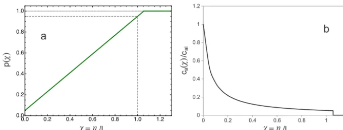
The above relation is illustrated in Fig. 7a with the sample evaluations

e

p0=0.05, pe1=0.95. (21)

Equations (20) and (21) are used in implementations of the MRSAA below. One way to develop forms of Eq. (19) that can show a wider variety of behavior than Eq. (20) would be through the performance of experiments similar to those of Chatanantavet and Parker (2008), but with a specific focus on various forms of macro-roughness that mimic those in the field.

The form for the derivative of Eq. (20) with respect toχ, which is given below, will prove useful in succeeding analy-sis.

df dχ =

 

 e

p1−ep0 . . .0≤χ≤ 1−_ep0 e p1−pe0

0 . . . χ > 1−ep0 e p1−pe0

(22)

a

b

bedrock exposed alluvium-covered bedrock

a/Lmr 0

1

1 K

K

K K

F

pF

p~

Lmr

0

bedrock exposed alluvium-covered bedrock

a/Lmr K F K

K

K_a

pF

p0

~

Lmr

0 1

1 b

0 1

1

pF

p0

~

a/Lmr K F K

K

K_a

p1

~

Lmr

b

completely alluviated bed

b

c

a

Figure 6.Illustration of the MRSAA model relation between areal fraction of alluvial cover of bedrock p(χ ) (green curves) and χ=ηa/Lmr, whereηais the thickness of alluvium (yellow fill) and Lmris the macro-roughness height, for (a) low cover, (b) interme-diate cover (c) complete alluviation above the top of the bedrock. The diagrams show alluvium–water interfaces at spatially constant elevations (blue lines). This is for illustrative purposes only: the in-terfaces should instead be those that result from averaging over an appropriate spatial window.

the condition that in the clast-rough case considered here, grain size is small compared to macro-roughness height. Fig-ure 6 also contains another simplification, in that all pockets are assumed to be filled to the same level by alluvium. While this condition is not likely to be true at the local scale, it is a reasonable first approximation when averaging over an ap-propriately defined window.

The formulation presented here has an obvious limitation. Since it is a 1-D expression of sediment conservation over a bedrock surface, it cannot capture 2-D variation, which will result in a more complex pattern than that shown in Fig. 6, and in particular will provide more connectivity between ad-jacent pockets. This two-dimensionality is known to have an effect on the pattern of incision, as illustrated by Johnson and Whipple (2007). The extension of the formulation to the 2-D case represents a future goal; some relevant comments can be found in the “Discussion” section (Sect. 8).

Sections 3.4 and 3.5, immediately below focus, on the mathematical interpretation of the MRSAA problem in terms of diffusion and wave characteristics. The reader whose primary interest is in applications may jump directly to Sect. 3.6, with the two exceptions of Eqs. (27) and (28) in Sect. 3.5. Equation (27) is a version of Eq. (6b) in which incisional morphodynamics are recast into a kine-matic wave equation, revealing upstream-migrating waves of incision with wave speedcb. Equation (28) is a version

of Eq. (18) in which alluvial morphodynamics are recast in terms of an advection–diffusion equation, with downstream-migrating waves of alluviation with speed ca, and alluvial

diffusion with kinematic coefficient of diffusionκa.

3.4 Character of the alluvial part of the MRSAA problem: alluvial diffusion and

downstream-migrating waves of alluviation

Equation (18) may be reduced to reveal the presence of an alluvial wave speed as follows. The derivative on the right-hand side of the equation is expanded using the chain rule, the derivative∂p/∂xis reduced in accordance with the gen-eral closure form of Eq. (19), and both sides of Eq. (18) are then divided bypto yield

∂ηa

∂t +ca ∂ηa

∂x = −

1 (1−λ)I

∂qac

∂x , (23a)

where

ca=

I (1−λ)

qac

Lmrp

df

dχ. (23b)

The left-hand side of Eq. (23a) thus takes a kinematic wave form, such thatcais the wave speed of downstream-directed

alluviation.

It is important to realize that alluvial wave speedca is a

nonlinear function of alluvial thicknessηa. Using the

exam-ple functions of Eqs. (20) and (22), the speedcaiof an alluvial

wave of infinitesimal heightηa=0 is given from Eq. (23b) as

cai=

I (1−λ)

qac

Lmr

(p_e1−pe0)

e

p0

. (24a)

The ratioca/caiof the wave speedcaat heightηato the

a/Lmr

 

a

p

 /c

ai

a

c



0 0.2 0.4 0.6 0.8 1 1.2

0 0.2 0.4 0.6 0.8 1 1.2

a/Lmr

 

b

Figure 7. (a) Simplest modified form the MRSAA cover function (green curve) satisfying the conditions p(0)=r, p(1)=1−r and p(∞)=1, where in this caser=0.05. The parameter on the vertical axisp(χ )denotes the cover fraction, and the parameter on the horizon-tal axis isχ=ηa/Lmr, whereηais the thickness of alluvium andLmris the macro-roughness height. (b) Plot of the ratio of alluvial wave speedca(χ )at a finite value ofχ=ηa/Lmrto the corresponding speedcai for an alluvial wave of infinitesimal height versusχ. The plot shows that alluvial wave speed declines with increasing alluvial thickness, and that it vanishes under complete alluviation.

ca

cai

=(pe1−ep0) e

p0

1 p

df

dχ. (24b)

In Fig. 7b, the ratio ca/cai is plotted against χ=ηa/Lmr

in accordance with the specifications of Eqs. (20), (21), and (22). It is seen therein that alluvial wave speed takes its maximum value for the limit ηa→0, and decreases to

a vanishing value as the bed becomes completely alluviated (ηa/Lmr=1.056). That is, waves of alluvium run fastest over

a nearly bare bed, and wave-like behavior ceases to exist un-der conditions of complete alluviation. This latter result is in accordance with Lisle et al. (2001) and Cui et al. (2003a, b). It is of interest to inquire as to how the model would be-have if the clast-rough condition, i.e.,Lmr/D1, were not

satisfied here. The limiting case of clast-smooth conditions would correspond to a probability distributionp(z_e 0)in Fig. 4 that obeys a step function;p(z_e 0)would be vanishing up to a smooth, horizontal bedrock surface, and would take the value unity above it. Consequently, the cover fractionpwould con-verge precisely to zero asηa→0, thus resulting, according

to Eq. (23b), in an infinite speed of propagation of an allu-vial wave of infinitesimal height. This is not entirely unreal-istic: the physical realization would consist of clasts rolling rapidly over a smooth bed with no alluviation (Inoue et al., 2014). The presence of such a singularity, would, however, preclude the modeling of the migration of a pulse of allu-vium of finite extent over the otherwise bare bed schematized in Fig. 3. In the present clast-rough formulation, the presence of deep pockets within the bedrock relief where alluvium can be stored without transport ensures that the wave speed of al-luvium never displays a singularity.

The form of Eq. (23a) can be further clarified by rewriting it as

∂ηa

∂t +ca ∂ηa

∂x −

∂ ∂x

κa

∂ηa

∂x

= ∂

∂x

κa

∂ηb

∂x

, (25)

where

κa=

I qac

(1−λ) S, (26a)

S= −∂η

∂x = −

∂ηb

∂x −

∂ηa

∂x. (26b)

In the above relation, κa has the physical meaning of a

kinematic diffusivity. In general,qac,qac/S and thusκa are

nonlinear functions of S. The alluvial problem thus takes the form of a nonlinear advective–diffusive problem with a source term arising from a bedrock term.

3.5 Full MRSAA formulation: alluvial diffusion, upstream-migration waves of incision, downstream-migrating waves of alluviation

The full MRSAA model consists of the kinematic wave equation with a source term Eq. (8a) for the bedrock part, Eqs. (23b), (25) and (26) for the alluvial part, and the linkage between the two embodied in the cover relation of Eq. (19). Restating these equations for emphasis, Eq. (6a) can be re-cast as

∂ηb

∂t −cb ∂ηb

∂x =υ, (27a)

cb=Iβqacp(1−p)

−∂ηb ∂x

−1

, (27b)

where cb denotes the speed of upstream-migrating

∂ηa

∂t +ca ∂ηa

∂x −

∂ ∂x

κa

∂ηa

∂x

= ∂

∂x

κa

∂ηb

∂x

, (28a)

ca=

I (1−λ)

qac

Lmrp

df

dχ, (28b)

df dχ =

dp d(ηa/Lmr)

, (28c)

κa=I (1−λ)qac

− ∂

∂x(ηa+ηb)

−1

(28d)

and

p=f (χ )=

 

 e

p0+(pe1−ep0) χ . . .0≤χ≤

1−p_e0

e p1−ep0

1 . . . χ > 1−ep0

e p1−ep0

,

(29)

wherecadenotes the speed of downstream-migrating alluvial

waves, andκais the kinematic diffusivity of alluvium. In this

way, upstream-migrating incisional waves are combined with downstream-migrating alluvial waves and alluvial diffusion. In MRSAA, then, the spatiotemporal variation in the cover fractionp(x, t )is specifically tied to the corresponding vari-ation in ηa through Eq. (19), e.g., the specific example of

Eq. (29) above. This variation then affects incision through Eq. (27). Consider the simplified case of a wave of alluvium of finite extent illustrated in Fig. 3. There is no incision up-stream of the wave becausep=0 and there is no sediment in motion over the bed. At the peak of the wave,ηa> Lmr, so

p=1; the bed is entirely covered with sediment, and again there is no incision. Incision can only occur on the rising and falling parts of the wave, where bedrock is partially exposed and sediment is in motion over it, i.e., 0< p <1. It can thus be expected that the spatiotemporal variation in cover thick-nessηawill affect the evolution of the long profile of an

in-cising river that undergoes transitions between alluvial and mixed bedrock–alluvial states.

3.6 Amendment of the flow component of the MRSAA model

The flow model, and in particular Eqs. (9a) and (11), must be modified to include the alluvial formulation, so that bedrock slopeSbis replaced with slopeSof the top of the bed, where

S= −∂η

∂x =Sb+Sa, (30a)

Sb= −

∂ηb

∂x, (30b)

Sa= −

∂ηa

∂x. (30c)

Thus Eqs. (9a) and (11a, 11b) are amended to

τ=ρgH S (31)

and

H=

_Q2

Cz2_gB2_S 1/3

, (32a)

τ∗=

Q2 Cz2_gB2

1/3

S2/3

RD. (32b)

The purely alluvial case, i.e., p=1, df/dχ=0 and ηb=const< ηa in Eq. (28), results in the purely diffusional

relation

∂ηa

∂t =

∂

∂x

κa

∂ηa

∂x

, (33)

in which the diffusivityκais a function ofSa= −∂ηa/∂x.

3.7 How the governing equations connect to each other

In the numerical analysis below, the actual equations used to solve for morphodynamic evolution are not those of Sects. 3.4 and 3.5, but rather the primitive forms presented earlier. The unknowns to be solved areηb,ηa,η,p,qac,τ∗,

S,Sb andSa. These nine parameters are connected to each

other via nine equations, i.e., Eqs. (5c), (6b), (12), (18), (20), (30a, b, c) and (32b).

3.8 Equivalence of the MRSAA and CSA models at steady state

In the restricted case of the highly simplified reach (HSR) configuration constrained by (a) temporally constant, below-capacity sediment feed (supply) rateqaf, (b) bedload

trans-port rateqa everywhere equal to the feed rateqaf, and (c) a

steady-state balance between incision and rock uplift,ηa,p

andSbbecome constant andSavanishes, so that Eq. (28) is

satisfied exactly. Equation (18) integrates to give

p=qaf qac

, (34)

so thatηacan then be back-calculated from Eq. (20). In this

case, then, the MRSAA model reduces to Eqs. (27) and (34), i.e., the CSA model.

4 The below-capacity steady-state case common to the CSA and MRSAA models

pss=1−ϕ, (35a)

ϕ= υ

I βssqaf

, (35b)

qacss=

qaf

pss

, (35c)

wherepss,βss andqacss denote steady-state values of p,β

andqac, respectively. Equations (35a)–(35c) describe a

bal-ance between the incision rate and relative vertical rock ve-locity (e.g., constant rock uplift rate at constant base level or constant rock elevation with constant rate of base level fall). CSA and MRSAA yield the same solution for this case, which must be characterized before showing how the models differ.

Equation (35a) has an interesting character. When the value of the dimensionless number ϕ exceeds unity, p falls below zero and no steady-state solution exists. Equa-tion (35b) reveals thatϕ can be interpreted as a dimension-less rock uplift rate. Thus when the rock uplift rate is suffi-ciently large forϕto exceed unity, incision cannot keep pace with rock uplift. The model thus implicitly predicts the for-mation of a hanging valley. This issue was earlier discussed in Crosby et al. (2007).

In solving for this steady state, and in subsequent calcu-lations, we use the bedload transport relation of Wong and Parker (2006a), a development and correction of the semi-empirical relation of Meyer-Peter and Müller (1948), rather than the similar formulation of Fernandez Luque and van Beek (1976); in the case of the former,αa=4,na=1.5 and

τ_c∗=0.0495. We consider two cases: one for whichβss=β

is a specified constant, and one for which only a reference valueβrefis specified, andβssis computed from Eq. (5d).

In the case of a specified constant abrasion coefficientβ, specification of υ, I and qaf allow computation of ϕ, pss

andqacssfrom Eqs. (35a)–(35c). Further specification ofR

(here chosen to be 1.65, the standard value for quartz) and Dallows the steady-state Shields numberτ_ss∗to be computed from Eq. (5c). Steady-state bedrock slope Sbss can then be

computed from Eq. (11b) upon specification of flood dis-chargeQ, Chézy resistance coefficientCzand channel width B. In the case of βss calculated according to Eq. (5d)

us-ing a specified reference value βref, the problem can again

be solved with Eqs. (35), (5c) and (11b), but the solution is implicit.

We performed calculations for conditions loosely based on (a) field estimates for a reach of the bedrock Shimanto River near Tokawa, Japan (Fig. 1), for which bed slopeSis about 0.002 and channel width is about 100 m and (b) es-timates using relations in Parker et al. (2007) for allu-vial gravel-bed rivers with similar slopes, and reasonable choices for otherwise poorly constrained parameters. The input parameters,Cz=10,Q=300 m3s−1,B=100 m, are loosely justified in terms of bankfull characteristics of allu-vial gravel-bed rivers of the same slope (Parker et al., 2007;

1 10 100

0.00001 0.0001 0.001 0.01 0.1 Cz

S

Grain Size < 0.062 mm 0.062 - 0.5 mm 0.5 - 2 mm 2 - 25 mm > 25 mm Shimanto (a)

1 10 100 1000 10000

0.1 10 1000 100000 10000000 Bbf[m]

Qbf[m3/s]

Grain Size < 0.062 mm 0.062 - 0.5 mm 0.5 - 2 mm 2 - 25 mm > 25 mm Shimanto (b)

a

b

104 105 10-5 10-4

104

Figure 8.(a) Chézy resistance coefficientCzplotted against bed slopeSfor alluvial rivers. Also included are estimated values for the Shimanto River, Japan. (b) Bankfull widthBbfversus bankfull dischargeQbf for alluvial rivers. Also included are estimates for bank-to-bank width and characteristic flood discharge in the Shi-manto River, Japan. The ranges for characteristic bed material size of the alluvial rivers are denoted in the legends.

Wilkerson and Parker, 2011) as shown in Fig. 8a and b. The value D=20 mm represents a reasonable characteris-tic size of the substrate (and thus the bedload) for gravel-bed rivers; a typical size for surface pavement is 2 to 3 times this (e.g., Parker et al., 1982). Flood intermittencyI is estimated at 0.05, i.e., 18 days per year, and thus a reasonable estimate for a river subject to frequent heavy storm rainfall. Alluvial porosity isλ=0.35.

Two sediment feed rates were considered. The high feed rate was set at 3.5×105t yr−1, which corresponds to the following steady-state parameters at capacity conditions: Shields numberτ∗=0.12, depthH=1.5 m, steady-state al-luvial bed slopeSass=0.0026 and Froude numberFr=0.51,

where

F r= Q

BH√gH. (36)

number τ∗=0.064, depth H=2.1 m, steady-state alluvial bed slopeSass=0.0010 and Froude numberFr=0.32.

The valueβss=0.05 km−1was used for the case of a

con-stant steady-state abrasion coefficient. This corresponds to a value ofαdof 0.017 km−1, which falls in the middle of the

range measured by Kodama (1994) for chert, quartz and an-desite (see Fig. 3-41 of Parker, 2008). For the case of a vari-able abrasion coefficient, Eq. (1a) was used withβrefset to

0.05 km−1andτ_ref∗ set to 0.12, i.e., the value for the high feed rate. This value ofτ_ref∗ is about 2.5 times the threshold value of Wong and Parker (2006a).

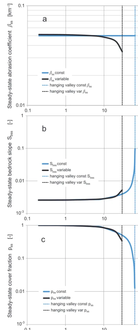
For the high feed, predicted relations for a steady-state abrasion coefficientβssversus rock uplift rateυare shown in

Fig. 9a; the corresponding predictions for Sbssversusυ are

shown in Fig. 9b; the corresponding predictions forpssand

ϕ are shown in Fig. 9c. Both the cases of constant and vari-able βss are shown. There are five notable aspects of these

figures: (a) in Fig. 9a, the predictions for variable βss are

very similar to the case of constant, specifiedβss, and indeed

are nearly identical for υ≤3.3 mm yr−1 (corresponding to ϕ≤0.05 in Fig. 9c). (b) In Fig. 9b and c, the predictions for Sbss,pss andϕfor variableβssare again nearly identical to

those for constantβss, and again essentially independent ofυ

forυ≤3.3 mm yr−1. (c) In Fig. 9c,pssis only slightly below

unity (i.e., pss≥0.95), and ϕ≤0.05 for υ≤3.3 mm yr−1).

(d) Forυ >3.3 mm yr−1, the predictions forSbssandpss

be-come dependent on υ, such thatSbssincreases, andpss

de-creases, with increasing υ. The values for constantβss

di-verge from those for variableβss, but are nevertheless close to

each other up to some limiting value. (e) This limiting value corresponds toϕ=1 and thuspss=0 from Eq. (35a); larger

values ofϕlead to hanging valley formation. Hereϕ=1 for the very high values υ=65 mm yr−1 _{for constant β}

ss and

υ=30 mm for variableβss.

These results require interpretation. It can be seen from Eqs. (35a–35c) that whenυ/(I βssqaf)=ϕ1,p becomes

nearly equal to unity (very little exposed bedrock), in which caseqafis constrained to be only slightly smaller than qac.

From Eqs. (5c) and (11), then, Sbss is only slightly above

the steady-state alluvial bed slopeSass. Note that the

steady-state bedrock slope decouples from rock uplift rate under these conditions: the predictions for υ=0.2 mm yr−1 are nearly identical to this forυ=3.3 mm yr−1. This behavior is a specific consequence of the condition ϕ1 correspond-ing to a low ratio of uplift rate to reference incision rate Eref=I βssqaf. They imply a wide range of conditions for

which (a) very little bedrock is exposed, and (b) bedrock slope is independent of uplift rate.

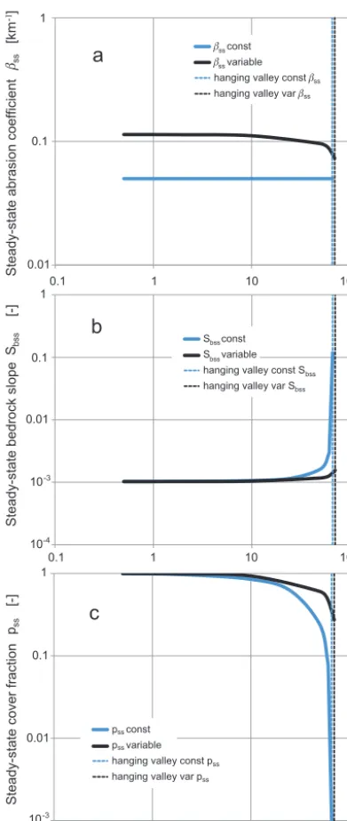
The results for the low feed rate are very similar. The values for variable steady-state abrasion coefficientβss

dif-fer from the constant value βss in Fig. 10a, but this is

be-cause the constant value βss=0.05 was set based on the

high feed rate. The results in Fig. 10b and c are qualita-tively the same for Fig. 9b and c; the uplift rate below which ϕ <0.05 is υ <0.33 mm yr−1 for the case of constantβss,

0.01 0.1 1

0.1 1 10 100

0.01 0.1 1

0.1 1 10 100

0.01 0.1

0.1 1 10 100

Rock uplift or base lowering rate  [mm/yr]

[k

m

-1]

ss

Steady-state abrasion coefficient

[-]

Steady-state bedrock slope

Sbs

s

[-]

Steady-state cover fraction

pss 10-3

10-3

c

b

a

S const S variable hanging valley const S hanging valley var S

bss

bss

bss bss

 const

 variable

hanging valley const 

hanging valley var 

ss ss

ss ss

p const p variable hanging valley const p hanging valley var p

ss ss

ss ss

0.01 0.1 1

0.1 1 10 100

0.01 0.1 1

0.1 1 10 100

0.01 1

0.1 1 10 100

Rock uplift or base lowering rate [mm/yr]

[k

m

-1]

ss

Steady-state abrasion coefficient

[-]

Steady-state bedrock slope

Sbs

s

[-]

Steady-state cover fraction

pss 0.1

10-4 10-3

10-3

 const  variable hanging valley const  hanging valley var 

ss ss

ss ss

c

b

a

p const p variable hanging valley const p hanging valley var p

ss ss

ss ss

S const S variable hanging valley const S hanging valley var S

bss bss

bss bss

Figure 10.Variation at steady state (black curves) of (a) abrasion coefficient βss, (b) bedrock slopeSbssand (c) cover fractionpss and parameterϕwith rock uplift or base lowering rateυ, for a low bedload feed rate of 3.5×104t yr−1. The cases of constant, spec-ifiedβssandSbssvarying according to Eq. (34) are shown as blue curves. The vertical dashed lines denote the incipient conditions for the formation of a hanging valley. The predictions are the same for the CSA and MRSAA models.

andυ <0.73 mm yr−1for the case of variableβss. The

crit-ical value of υ beyond which a hanging valley forms is υ≥6.8 mm yr−1 _{for constant β}

ss and υ≥7.1 mm yr−1 for

variableβss.

The lack of dependence of steady-state bedrock slopeSbss

on rock uplift rateυbelow a threshold value for the steady-state solutions of the CSA model (and thus the MRSAA model as well) is in stark contrast to earlier work for which the incision rateEis assumed to have the following depen-dence on slopeSband drainage areaA(“slope–area”

formu-lation, Howard and Kerby, 1983):

E=KS_bnAm, (37)

whereAdenotes drainage area,nandmare specified expo-nents, andKis a constant assumed to decrease with increas-ing rock hardness.

In order to compare the steady-state predictions of the slope–area relation in Eq. (37) for constant υ with CSA, drainage areaAmust be taken to be a constant valueAoso

as to correspond to the HSR configuration used here. The steady-state slopeSbss corresponding to a balance between

incision and rock uplift is found from Eq. (37) to be

Sbss=

υ1/n

K1/n_Am/n

o

. (38)

The issue as to the values ofmandnhas been considered by many researchers, including Whipple and Tucker (2002) and Lague (2014).

In their Table 1, Whipple and Tucker (2002) quote a range of values ofn, but their most quoted value isn=2. We com-pare the results for CSA forSbss with the predictions from

Eq. (38) withn=2 by normalizing against a reference value Sbref that corresponds to a reference rock uplift rateυref of

0.2 mm yr−1. Equation (38) yields

Sbss

Sbref

=

_υ

υref 1/2

. (39)

In Fig. 11, Eq. (39) is compared against the CSA predictions of Figs. 9b and 10b (high and low feed rate, respectively) for both constant and variableβss. In order to keep the plot

within a realistic range, only values ofυ between 0.2 and 10 mm yr−1(the upper limit corresponding to Dadson et al., 2003) have been used in the CSA results. The remarkable in-sensitivity of the CSA predictions for steady-state slopeSbss

0 1 2 3 4 5 6 7 8

1 10 100

Sbss /Sbref

Steady-state bedrock slope

/ ref

 

Normalized uplift rate high feed  const high feed  variable low feed  const low feed  variable slope-area model

Figure 11.Normalized steady-state bedrock slopeSbss/Sbref ver-sus normalized rock uplift rateυas predicted by the CSA model for a low feed rate (orange-brown curves) and a high feed rate (black curve and dashed red curve), and for constant and variable abra-sion coefficient. The results are the same for the MRSAA model. Also shown is the prediction of a model for which the incision rate is specified in terms of bedrock slope and upstream drainage area (green curve). Note that the predictions for steady-state bedrock slope of the CSA model are insensitive to the rock uplift rate over a wide range.

5 Boundary conditions and parameters for numerical solutions of the MRSAA model

Having conducted a fairly thorough analysis of the steady state common to the CSA and MRSAA models, it is now ap-propriate to move on to examples of behavior that can be cap-tured by the MRSAA model, but are not capcap-tured by models that assume a relation for cover based on the ratio of sediment supply to capacity transport rate, i.e., Eq. (2). Before doing so, however, it is necessary to delineate the boundary condi-tions and other assumpcondi-tions used in the MRSAA model.

LetLdenote the length of the reach. Equation (27a) indi-cates the formulation for bedrock incision is first order inx and so requires only one boundary condition. The example considered here is that of a downstream bedrock elevation, i.e., base level, set to zero:

ηb|x=L=0. (40)

According to Eq. (18), or alternatively Eq. (28a), the allu-vial formulation is second order inx and thus requires two boundary conditions. The following boundary condition ap-plies at the upstream end of the reach, whereqaf(t) denotes a

feed rate that may vary in time,

qa|x=0=qaf(t ). (41)

At the downstream end, a free boundary condition is applied forηa/Lmr<1, and a fixed boundary condition is applied for

ηa/Lmr≥1 as follows:

(1−λ)p∂ηa ∂t +I

∂pqac ∂x

x=L

=0 . . .if

_η

a Lmr

x=L

<1, (42a)

ηa|x=L=Lmr . . .if

_η

a Lmr

x=L

≥1. (42b)

Here, Eq. (42a) specifies a free boundary in the case of partial alluviation, thus allowing below-capacity sediment waves to exit the reach. Equation (42b), on the other hand, fixes the maximum downstream elevation atη=ηa=Lmr.

In order to illustrate the essential features of the new for-mulation of the MRSAA model for the morphodynamics of mixed bedrock–alluvial rivers, it is useful to consider the most simplified case that illustrates its expanded capabilities compared to the CSA model. Here we implement the HSR simplification. In addition, based on the results of the pre-vious section, we approximateβssas a prescribed constant.

Finally, we assume that the clasts of the abrading bedload are sufficiently hard compared to the bedrock so that grain sizeDcan be approximated as a constant. These constraints are easily relaxed.

In the numerical solution of the differential Eqs. (6b) and (18), spatial derivatives have been computed using an upwinding scheme for short timescales (so as to capture downstream-migrating alluvial waves) and a downwinding scheme for long timescales (so as to capture upstream-migrating incisional waves). Time derivatives have been computed using the Euler step method.

6 Sediment waves over a fixed bed: stripping and emplacement of alluvial layer and

advection–diffusion of a sediment pulse

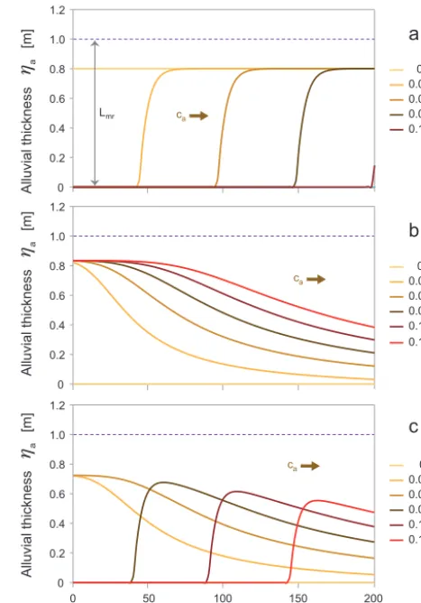
Three numerical solutions of the MRSAA model are stud-ied here: (a) stripping of an alluvial cover to bare bed, (b) emplacement of an alluvial cover over a bare bed and (c) advection–diffusion of an alluvial pulse over a bare bed. Reach lengthLis 20 km. As the time for alluvial response is short compared to incisional response,βssandυare set equal

to zero for these calculations. In addition, flood intermittency Iis set to unity so as to illustrate the migration from the feed point to the end of the reach under the condition of contin-uous flow. The macro-roughnessLmris set to 1 m based on

observation of the Shimanto River near Tokawa, Japan. The values forCz,Q,B, D and λ are the same as in Sect. 5, i.e.,Cz=10, Q=300 m3s−1_{,B=100 m, D=20 mm and}

λ=0.35. Bedrock slopeSb, which is constant due to the

None of these three cases can be treated using models that assume a relation for cover based on the ratio of sediment supply to capacity transport rate, i.e., Eq. (2). They thus il-lustrate capabilities unique to MRSAA.

6.1 Alluvial stripping

The case of stripping of an initial alluvial layer to bare bedrock is considered here. In this simulation, the bedload feed rate qaf=0 and the initial thickness of alluvial cover

ηa is set to 0.8 m, i.e., 80 % of the macro-roughness length

Lmr. To drive stripping of the alluvial layer, the feed rate is

set equal to zero. Figure 12a shows how the alluvial cover is progressively stripped off from upstream to downstream as a wave of alluvial rarification migrates downstream. The al-luvial layer is completely removed (except for residual sed-iment in deep pockets, as specified by Eq. 21) after a little more than 0.12 years.

Of interest in Fig. 12a is the fact that the wave of strip-ping maintains constant form in spite of the diffusive term in Eq. (28a) which should cause the wave to spread. The rea-son the wave does not spread is the nonlinearity of the wave speed ca in Eq. (28b): sincep enters into the denominator

on the right-hand side of the equation, wave speed is seen to increase as pdecreases, and thusηadecreases. As a result,

the lower portion of the wave tends to migrate faster than the higher portion, sharpening the wave and opposing diffusion.

6.2 Emplacement of an alluvial layer over an initially bare bed

In this simulation, the initial thickness of alluvium ηa is set

to zero and the sediment feed rate is set to 0.0013 m2_s−1_,

i.e., 80 % of the capacity value. The result of the calculation is shown in Fig. 12b. Here nonlinear advection and diffusion act in concert to cause the wave of alluviation to spread. The steady-state thickness of alluvium is 0.83 m; by 0.1 years it has been emplaced only down to about 5 km from the source. This steady-state condition, and only this condition, corre-sponds to a convergence of results from MRSAA and CSA.

6.3 Propagation of a pulse of alluvium over an initially bare bed

In this example the initial bed is bare of sediment. The sed-iment feed rate is set equal to 0.0012 m2s−1, i.e., 70 % of the capacity value for 0.05 years from the start of the run, and then dropped to zero for the rest of the run. Figure 12c shows the propagation of a damped alluvial pulse through the reach, with complete evacuation of the pulse in a little more than 0.15 years. Nonlinear advection acts against diffusion to suppress the spreading of the upstream side of the pulse, but advection acts together with diffusion to drive spreading of the downstream side of the pulse.

ca

0 yr 0.03 yr 0.06 yr 0.09 yr 0.12 yr Lmr

0 0.2 0.4 0.6 0.8 1.0 1.2

Downstream distance x [km]

Alluvial thickness

a



[m]

ca

0 0.2 0.4 0.6 0.8 1.0 1.2

0 0.2 0.4 0.6 0.8 1.0 1.2

0 50 100 150 200

0 yr 0.02 yr 0.04 yr 0.06 yr 0.10 yr

0 yr 0.025 yr 0.050 yr 0.075 yr 0.100 yr 0.125 yr

Alluvial thickness

a



[m]

Alluvial thickness

a



[m]

ca

0.12 yr a

b

c

Figure 12.MRSAA model solutions for (a) stripping of an allu-vial layer to bare bedrock, (b) emplacement of an alluallu-vial cover over initially bare bedrock and (c) evolution of a pulse of sediment over bare bedrock. Numerical simulations of the evolution of allu-vial thicknessηa(x, t )over streamwise distancexare shown for a series of time stepstas indicated in the legends.

7 Comparison of evolution to uplift-driven steady state for the CSA and MRSAA models

7.1 Evolution of bedrock profile with early-stage massive alluviation

Here we set Q, B, Cz, D and λ to the same values as Sect. 6. The reach lengthLis 20 km, the flood intermittency I is set to 0.05, macro-roughnessLmr is set to 1 m, initial

alluvial thicknessηa|t=0=0.5 m, downstream bed elevation

ηb|x=L=0 and the abrasion coefficient βss is 0.05 km−1.

The initial bed slope is 0.004. The feed rate is set to twice the capacity rate for this slope, i.e.,qaf=0.0033 m2s−1. The

up-lift rate is set to the very large value of 5 mm yr−1. It should be noted, however, that as shown in Fig. 10b, the steady-state bedrock slope for this feed rate is independent of the uplift rate forυ≤5 m yr−1_{. This is because the steady-state value}

ofϕis 0.019, i.e.,ϕ1.

The results for the CSA model are shown in Fig. 13a. The bed slope evolves from the initial value of 0.004 to a final steady-state value of 0.0068. Evolution is achieved solely by means of an upstream-migrating knickpoint. Only the first 4000 years of evolution are shown in the figure.

Figure 13b shows the results of the first 400 years of the calculation with MRSAA. By 100 years, the bed is com-pletely alluviated, and by 400 years, the thickness of the al-luvial layer at the upstream end of the reach is 52 m. This massive alluviation is, unsurprisingly, not predicted by CSA, which was designed to treat incision only. Figure 13c shows the results of the first 4000 years of evolution. The upstream-migrating knickpoint takes the same form as CSA, but it is nearly completely hidden by the alluvial layer. The knick-point gradually migrates upstream, driving the completely alluviated layer out of the domain, but this process is not complete by 4000 years. A comparison of Fig. 13a and c show that a knickpoint that is exposed in CSA is hidden in MRSAA. Models that assume a relation for cover based on the ratio of sediment supply to capacity transport rate cannot predict the presence of a hidden knickpoint.

7.2 Evolution of horst–graben configuration

In this example,Cz,Q,B,D,λ,I,βss,Lmr,L, ηa|t=0and

ηb|x=Lare set to the values used in Sect. 7.1. The sediment feed rateqaf=0.00083 m2s−1, and the initial bedrock slope

Sb is set to the steady-state value for a rock uplift rate of

1 mm yr−1, i.e., 0.0027. The model is then run for a rock uplift rate of 1 mm yr−1 for the domains 0≤x≤8 km and 12 km≤x≤20 km and a rock subsidence rate of 1 mm yr−1

for the domain 8 km< x <12 km. This configuration corre-sponds to a simplified 1-D configuration of a graben bounded by two horsts, one upstream and one downstream.

This case cannot be implemented in models that assume a relation for cover based on the ratio of sediment supply to capacity transport rate, i.e., Eq. (2). This is because such models are not designed to handle the case of alluvial fill of accommodation space created by subsidence. The results for MRSAA are shown in Fig. 14. By 15 kyr, the uplifting

0 20 40 60 80 100 120 140

knickpoint

xk(t)



[m]

Bedrock elevation

upstream-migrating

0 yr 800 yr 1600 yr 2400 yr 3200 yr 4000 yr

b

bedrock

a

Elevation

b

,





0 20 40 60 80 100 120 140

0 yr 400 yr

_b

bedrock

aggadation over bedrock

0 yr 100 yr 200 yr 300 yr 400 yr

top bed 

b

Elevation

b

,





0 20 40 60 80 100 120 140

0 50 100 150 200

Downstream distance x [km]

c

long term

top bed 

0 yr 800 yr 1600 yr 2400 yr 3200 yr 4000 yr

b

bedrock

alluvium

knickpoint upstream-migrating hidden

xk(t)

xk(t)

Figure 13.Progression to steady state after an impulsive increase in sediment supply: (a) CSA model; (b) MRSAA model, early stage; and (c) MRSAA model, late stage. Note the knickpointsxk(t )in bedrock in (a) and (b) and hidden in a migrating alluvial–bedrock transition in (c). Hereηdenotes elevation of the top bed surface, ηbdenotes elevation of the base of bedrock relief, andxdenotes streamwise distance. The retreating alluvial wedge is shaded in (c) for emphasis.