https://doi.org/10.5194/os-14-41-2018
© Author(s) 2018. This work is distributed under the Creative Commons Attribution 3.0 License.
Note on the directional properties of meter-scale gravity waves
Charles Peureux1, Alvise Benetazzo2, and Fabrice Ardhuin1
1Laboratoire d’Océanographie Physique et Spatiale, Univ. Brest, CNRS, Ifremer, IRD, 29200 Plouzané, France 2Institute of Marine Sciences, Italian National Research Council, Venice, Italy
Correspondence:Charles Peureux ([email protected]) Received: 2 June 2017 – Discussion started: 27 June 2017
Revised: 17 November 2017 – Accepted: 20 November 2017 – Published: 22 January 2018
Abstract.The directional distribution of the energy of young waves is bimodal for frequencies above twice the peak fre-quency; i.e., their directional distribution exhibits two peaks in different directions and a minimum between. Here we an-alyze in detail a typical case measured with a peak frequency
fp=0.18 Hz and a wind speed of 10.7 m s−1using a stereo-video system. This technique allows for the separation of free waves from the spectrum of the sea-surface elevation. The latter indeed tend to reduce the contrast between the two peaks and the background. The directional distribution for a given wavenumber is nearly symmetric, with the angle dis-tance between the two peaks growing with frequency, reach-ing 150◦at 35 times the peak wavenumberkpand increasing up to 45kp. When considering only free waves, the lobe ratio, the ratio of oblique peak energy density over energy in the wind direction, increases linearly with the non-dimensional wavenumberk/kp, up to a value of 6 atk/kp'22, and possi-bly more for shorter components. These observations extend to shorter components’ previous measurements, and have im-portant consequences for wave properties sensitive to the di-rectional distribution, such as surface slopes, Stokes drift or microseism sources.
1 Introduction
Directional properties of waves shorter than the dominant scale play a very important role in many aspects that range from air–sea momentum fluxes (Plant, 1982) to remote sens-ing, surface drift (Ardhuin et al., 2009) and underwater acoustics (Duennebier et al., 2012). In a landmark paper, Munk (2009) analyzed the linear trends of down-wind and cross-wind mean square slopes of the sea surface, as mea-sured by satellites Bréon and Henriot (2006). These trends
cannot be explained by today’s understanding of ocean wave spectra, and he proposed that there may be localized sources that could generate oblique propagating waves looking like ship wakes. However, as he put it, the dataset “says nothing about time and space scales” because the reflectance mea-surements that they present are integrated across all wave scales. Munk further challenged us all: “I look forward to in-tensive sea-going experiments over the next few years demol-ishing the proposed interpretations”. We thus went out to sea with the objective of resolving space scales and timescales, and providing further constraints on the wave properties.
Previous time-resolved measurements of ocean waves have clearly established a prevalence of directional bimodal-ity at frequencies above twice the peak frequencyfp, using in situ array (Young et al., 1995; Long and Resio, 2007) and buoy data (Ewans, 1998; Wang and Hwang, 2001). These were confirmed by airborne remote sensing techniques used by Hwang et al. (2000) and Romero and Melville (2010). All the resolved wavenumber spectra have been limited to
42 C. Peureux et al.: Short gravity wave directional distribution
The distribution of radar backscatter as a function of az-imuth clearly shows that the directional wave spectrum is unimodal above 6 cm wavelength in the gravity-capillary range (see the review in Elfouhaily et al., 1997). Recent backscatter data in L-band presented by Yueh et al. (2013) show a larger cross-wind than down-wind backscatter, con-sistent with a bimodal distribution at scales around 1 m wave-length, at least for wind speeds around 5 m s−1.
As shown by Leckler et al. (2015), stereo-video imagery is capable of resolving these waves and providing information on the timescales and space scales needed to interpret inte-grated wave parameters such as down-wind and cross-wind mean square slopes. In that earlier paper, a record with young wind waves was analyzed (U23=13.2 m s−1,fp=0.33 Hz). That record revealed the presence of second-order harmon-ics and a strong bimodality of the directional distribution. Here we use the same measurement method and analyze the directional properties of the free waves in more detail. In particular, we analyze new data that provide a wider range of frequencies and quantitatively characterize the bimodality characteristics together with its impacts on several physical variables.
The data and analysis methods are presented in Sect. 2. Directional distributions and bimodality are described in Sect. 3. Discussions and conclusions follow in Sect. 4.
2 Wave measurements and spectral analysis 2.1 Stereo processing
We have chosen one typical stereo record with dominant waves longer than those described in Leckler et al. (2015). It was acquired on 10 March 2014, starting at 09:40 UTC, from the Acqua Alta oceanographic research platform, 15 km offshore of Venice, Italy, in the northern Adriatic Sea. The mean water depth there is approximatelyd=17 m. The ex-perimental setup has been described in detail in Benetazzo et al. (2015). It is made up of two digital cameras mounted on a horizontal bar, properly synchronized and calibrated. The cameras are located d=12.5 m above the mean sea level. The stereo device points in a direction oriented 46◦ clock-wise from geographical north, i.e., looking to the northeast. The cameras’ elevation angle is 50◦. This record is 30 min long and uses a 15 Hz sampling rate.
In the following all variables use the meteorological con-vention; that is, the directions are directions from which wave, wind and current come. Provenance directions, unless otherwise specified, are measured anticlockwise from the di-rection along the bar, i.e., 136◦clockwise from geographical north.
The mean wind speed measured at 10 m above sea level is 10.7 m s−1, with mean directionθU=77◦(northeasterly).
The significant wave height estimated from the stereo system isHm0=1.33 m, with peak frequencyfp=0.185 Hz,
corre-sponding to a dominant wavelength on the order of 45 m. We note that wave gauges on the platform give independent measurements ofHm0=1.36 m andfp=0.189 Hz. Domi-nant waves and shorter components of the wave spectrum can be considered deep water waves. An acoustic Doppler current profiler (ADCP) deployed at the sea floor provides measurements of the horizontal current vector with a vertical resolution of 1 m.
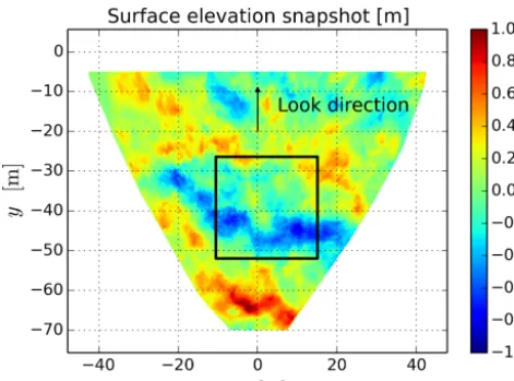
The raw video images are processed into a three-dimensional surface elevation matrixζ (x, y, t )following the method of Benetazzo et al. (2015). A local Cartesian refer-ence frame is defined, in which the surface elevation is re-constructed, with horizontal axesxandy. By convention, the cameras’ look direction is they axis, increasing away from the cameras, and thex axis is perpendicular, increasing to-wards the right of the cameras. The sea surface is discretized with a pixel size1x=1y=20 cm. A snapshot of the re-constructed sea-surface elevation map is presented in Fig. 1. We have selected a 25.6 m by 25.6 m area for Fourier anal-ysis, delimited by a black square. Its location, close to the cameras, is chosen to minimize errors in the estimate of the surface elevation. These errors increase with increasing dis-tance from the cameras, and are dominated by the quantiza-tion error (Benetazzo, 2006). Wavelengths longer than 25 m can be resolved using standard slope array techniques (e.g., Graber et al., 2000) as done by Leckler et al. (2015). These longer components are not the focus of the present paper.
All of our analysis is based on a three-dimensional power spectral density of these data (Figs. 2 and 3). This is ob-tained by applying a Hann spatiotemporal window with 50 % overlap in time, and averaging the spectra in time following Welch (1967). The frequency resolution is1f=0.015 Hz. The double-sided Cartesian spectrumE(kx, ky, f )is normal-ized so that
E=
Z Z Z
dkxdkydf E(kx, ky, f ) (1)
is the variance of the surface elevation.
The polar spectrum is more convenient for the study of di-rectional distributions and for working at a given wavenum-ber. The single-sided polar spectrum is
E(k, θ, f )=2kE(kx, ky, f ), (2)
wherek=(kx2+k2y)1/2andθ=arctan(ky, kx)+πis the wave provenance direction. For convenience, we use a regular po-lar grid whose resolution is set to 1k=0.17 rad m−1 and
1θ=1◦.
2.2 General properties of the three-dimensional spectrum
The surface elevation spectrum can be interpreted as the dis-tribution of wave energy, which can generally be divided into free and bound waves,
Figure 1.Stereo-video reconstructed sea-surface elevation matrix snapshot and sea-surface area used for spectrum calculations (black square).
Free waves have a relation between wavenumber and fre-quency that closely follows the linear dispersion relation. In the presence of a horizontally homogeneous and stationary current vertical profileu(z), and in the limit of small wave steepness, this dispersion relation is given by Stewart and Joy (1974):
ω(k,U)=σ (k)+kU (k)cos(θ−α), (4) where
σ (k)=pgktanh(kd) (5)
and the effective currentU (k)is approximated by a weighted integral of the Eulerian currentu(z)over the water column:
U (k)=2k
0
Z
−∞
u(z)e2kzdz. (6)
Here we have assumed that the current has a constant di-rection α at all depths. Moreover, Eq. (6) holds only for linear waves, i.e., waves for which hydrodynamic nonlin-earities have been neglected, although free waves may en-compass some weakly nonlinear contributions – see Leck-ler et al. (2015) and Janssen (2009). The depth weighting in the integral of Eq. (6) gives a stronger influence of sur-face currents on shorter wave components. In practice, waves with wavenumberkfeel the integrated current over a depth ∼1/ k. For convenience, the inverse function providing the wavenumber as a function of frequency and direction will be denotedκin the following, namely by definition: if
k=κ(f,U), (7)
then
2πf=ω(k,U), (8)
wheref= [fcos(θ ), fsin(θ )].
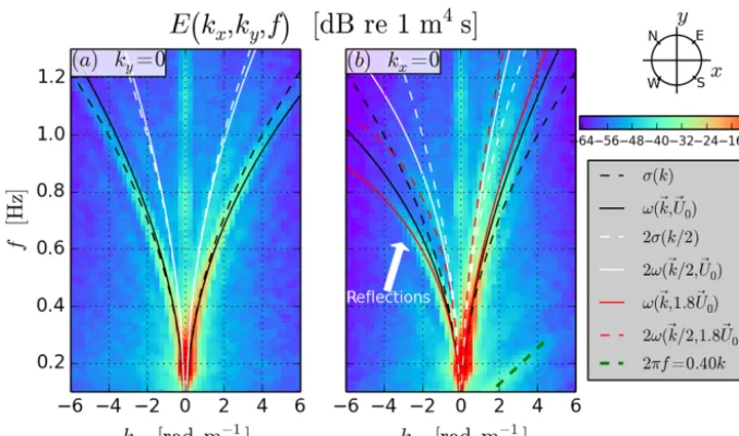
Once the effective current (Eq. 6) is known, the location of free waves in the(k, f )plane can be deduced from Eq. (4), which relates the radian frequency 2πf to the wave vector k. It is represented in Figs. 2 and 3 by a black solid line. The addition of a current is necessary to fit the observations of energy distribution. The free modes’ bimodality is clearly visible, i.e., the fact that two energy patches detach progres-sively from a main direction as the wave scale decreases.
Bound waves are dominated by the second-order in-teraction of free components with wavenumbers k1 and k2. The sum interaction gives waves of wavenumber k= k1+k2, and frequencyω=ω(k1)+ω(k2), with an energy
Esum. The difference interaction givesk=k1−k2andω= |ω(k1)−ω(k2)|,Ediff. These two kinds of interactions have themselves distinct signatures in the surface elevation spec-trum, namely
Ebound(k, f )=Esum(k, f )+Ediff(k, f ) . (9) At a given propagation direction, the sum interaction is found at frequencies higher than the dispersion surface, while the difference interaction components are found at lower fre-quencies (Leckler et al., 2015; Krogstad and Trulsen, 2010).
Eboundcan be deduced fromEfree(Hasselmann, 1962). More specifically, for a narrow spectrum, the sum interaction com-ponent is characterized by a signature in the (k, f ) plane (Senet et al., 2001)
2πf =2ω(k/2,U), (10)
also referred to as the first harmonic. The latter corresponds to sum interactions of free waves traveling in the same di-rection, with the same frequency and propagation didi-rection, for which the interaction cross section is highest (Aubourg and Mordant, 2015). This curve is represented in Figs. 2 and 3 by a white solid line. Its equivalent without a current is also plotted as a white dashed line. Nonlinear components do not exhibit the same directionality as linear waves in gen-eral, especially from snapshots at constant frequency. In this case, the harmonic peaks in the dominant wave direction (see Fig. 3b–f), although this is not the only possible behavior.
We also note that waves that are probably reflected by the platform legs are present, as shown by a white arrow in Fig. 2b, and their energy decreases with increasing dis-tance. When interpreted as plane waves, the reflected com-ponents appear slightly off the dispersion relation of the in-cident waves. Fitting the current for the inin-cident waves gives
U'0.22 m s−1, whereas a fit for the reflected components only would give a current velocity of 0.4 m s−1.
Finally, there are other spectral features that do not corre-spond to surface waves, which we shall call noise. We dis-tinguish four kinds of noise. Firstly, a background noise is present below−50 dB, particularly visible in Fig. 3d–f and j–l. This noise practically limits the use of stereo video to
44 C. Peureux et al.: Short gravity wave directional distribution
Figure 2.Frequency–wavenumber surface elevation spectrum at Acqua Alta on 10 March 2014 in dB and various dispersion lines. Spectrum along the cross-look(a)and look direction(b). The current used here,U0, is evaluated in the Appendix.
of 0.4 m s−1along the look direction and at slower speeds for other directions (green dashed lines in Figs. 2b and 3i–n). For
k=2 rad m−1this noise amplitude is comparable in magni-tude to the free wave signature and is distributed around a surface of the type 2πf=0.4sin2(θ )k, forθ∈ [0;π[only. It could be associated with the difference interaction between incident and reflected wavenumbers.
Besides these noises, uncertainties in the spectral densities are caused by the poor spectral resolution close tok=0, and quantization error noise, mostly for k >7.5 rad m−1and in the look direction (Benetazzo, 2006). We thus exclude from our analysis the spectral components for which any of the following conditions is met
f ≤1f, (11)
f >1.4 Hz, (12)
k≤1k, (13)
k >7.5 rad m−1, (14)
2πf[Hz]<1.1×0.4×sin2(θ )k[rad m−1]. (15) Outside of these components the spectrum is separated into free and bound components. This uses a determination of the effective current that is discussed in the Appendix. Identifying the free wave energy as that close to the linear dispersion relation, the bound components are defined as the rest,
Ebound(k, θ )=E(k, θ )−Efree(k, θ ), (16) and the same is done for the frequency–direction spectrum.
3 Directional properties of free waves
The spectrum of free waves Efree(k, θ ) is clearly bimodal fork >4kp. Bimodal energy distributions can be character-ized from the knowledge of the position and height of the energy peaks. The processing starts from the radially inte-grated directional distributions, both at a given frequency
Efree(θ )=Rdk Efree(k, θ ) and wavenumber Efree(θ )=
R
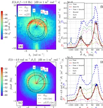
df Efree(f, θ ) (see Fig. 4). The same processing is per-formed on bound waves, obtained from Eq. (16). Bound waves are found to stand for a significant proportion of the overall energy at given slices (62 and 64 % on panels b and d, respectively), but only the free waves are bimodal. The energy level of bound waves at these small scales is domi-nated by the contribution of the more energetic longer waves. The contributions of the sum and difference interactions are also indicated. Directional distributions are centered on the spectral mean direction of wave propagationθm=68◦from Benetazzo et al. (2015).
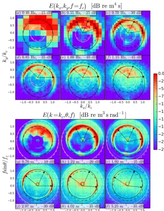
Figure 3.Surface elevation spectrum at Acqua Alta (continued).(a)to(f): Cartesian spectrum at constant frequenciesfc.(g)to(l): Cartesian spectrum interpolated into polar coordinates at constant wavenumberskc=κ(fc,0). The reference levels are indicated in the text boxes. The arrows point to the directions of the two peaks of the bimodal distributions (outer arrows) and to the central minimum (inner arrow). See legend in Fig. 2 for the various meanings of the lines.
Efit(θ )=Cst+f (θ;A1, µ1, σ1, x1)
+f (θ;A2, µ2, σ2, x2), (17) where
f (θ;A, µ, σ, x)=(1−x)A
σg
√ 2π e
−(θ−µ)2/2σ2
g
+xA
π
σ
(θ−µ)2+σ2, (18)
withσg=σ/
√
2 ln 2. The use of a double Voigt profile does not strictly ensure a smooth periodic distribution (around
θ=θm±π). However, in practice, due to the relative direc-tional narrowness of the bimodal profiles, the constant energy floor is quickly reached away from the mean wave propaga-tion direcpropaga-tion. Bimodality can then be characterized using a set of three remarkable points in the double Voigt profile (see Fig. 4b, d) (Wang and Hwang, 2001), i.e., the central mini-mum(θ0, E0)and the two peaks(θ1, E1)and(θ2, E2), with
θ1< θ2.
4 Results
46 C. Peureux et al.: Short gravity wave directional distribution
Figure 4. Free wave extraction(a, c)and corresponding directional distributions (b, d). Left panels: semi-automatic extraction of free waves, withαthe current direction,θmthe spectral mean direction of wave propagation andθU the wind direction. Right panels: directional
distributions of free waves (solid line), with fits and the various nonlinear contributions.
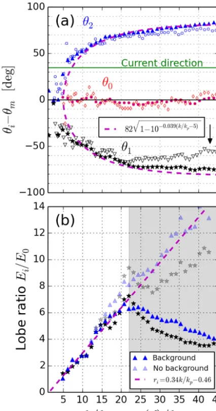
function of normalized wavenumberk/kp(see Fig. 5). Full markers (triangles, disks and stars) correspond to estimates from constant wavenumber snapshots, while empty markers (circles, diamonds and upside down triangles) correspond to estimates from constant frequency snapshots. For the latter, thex-axis isκ(f )/kp– see Eq. (7). Bimodal profiles are first detected atf =0.43 Hz andk=0.7 rad m−1, corresponding approximately tok/kp=5. The previously mentioned direc-tion θm is the best compromise for centering the bimodal-ity. An empirical parametrization is found for the constant wavenumber estimates of the directional distributions, that is,
(θ−θm)[◦] =82
q
1−10−a(k/kp−5), (19)
where the valuea=0.039 was found after a least squares fit of constant wavenumber data points in the range 5< k/kp< 45. This parametrization fits most of the measurements, ex-cept the position of the peak furthest from the current di-rection (θ1), particularly for the estimates from constant
fre-quency snapshots abovek/kp=22 (see the black arrow in Fig. 5). At this location, the peak is progressively moved to-wards the center of the directional distribution.
The lobe ratiosri are conventionally defined as the ratios
of the energy of each peak of the bimodal directional distri-bution to the one of the central minimum (Wang and Hwang, 2001), namely
ri = Ei E0
, i=1,2. (20)
We can note that they are particularly sensitive to the back-ground energy level. This level is given by the constant term
con-Figure 5. Bimodal directional distribution characteristics from stereo video as a function of normalized wavenumber. (a) Peak positions.(b)Lobe ratios. Empty markers correspond to constant frequency estimates and full markers to constant wavenumber esti-mates (see Fig. 4 for definitions).
stant frequency estimates exhibit a more pronounced asym-metry. A fit is performed over constant wavenumber lobe ra-tios (full markers) for which 4< k/kp<22, providing the parametrization
ri =0.34k/kp−0.45. (21)
Abovek/kp'22, the lobe ratios progressively decrease, ex-cept if the background termCst>0 is removed (transparent markers in Fig. 5). The lobe ratio decrease is natural since the lobe ratios without background are
ri0=Ei−C st
E0−Cst
> ri (22)
as long asri>1 and the proportion of background noise in-creases towards shorter scales. We cannot however formally associate this noise with an actual surface wave signal.
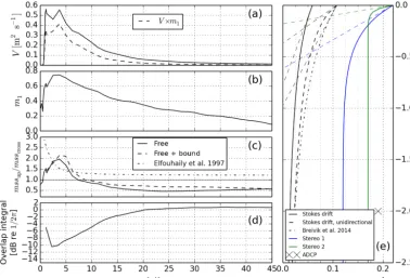
The Stokes drift current for linear waves in deep water is (Kenyon, 1969)
us(z)= ∞
Z
0
dk V (k) m1(k) e2kz, (23)
where
V (k)=2σ (k) kEfree(k) (24)
is plotted in Fig. 6a, and where the impact of the wave field directionality is included in the factor
m1(k)=
q
a12+b12, (25)
plotted in Fig. 6b with
a1(k)= 2π
Z
0
dθ Mfree(k, θ )cos θ− ¯θ (26)
and
b1(k)= 2π
Z
0
dθ Mfree(k, θ )sin θ− ¯θ (27)
the Longuet-Higgins coefficients with respect to the mean wave propagation direction, where
E (k, θ )=M (k, θ ) E (k) (28)
and 2π
Z
0
M (k, θ ) dθ=1. (29)
The resulting Stokes drift vertical profile has been plotted in Fig. 6e, together with two profiles compatible with the ef-fective current measured from stereo video (see Appendix). Waves slightly shorter than peak waves are the main contrib-utors to the Stokes drift (Fig. 6a). Half of the Stokes drift is carried by waves with frequencies greater than 0.4 Hz ap-proximately (wavelength 10 m). In order to correct for the stereo device field of view limitation (long waves are indeed not spatially resolved), the wavenumber spectrum fork < 1k
48 C. Peureux et al.: Short gravity wave directional distribution
Figure 6.Short wave contribution to various sea state variables.(a)Spectrum of non-directional Stokes drift, Eq. (24).(b)Stokes drift directional correction, Eq. (23).(c)Mean square slope up-wind over cross-wind ratio, Eqs. (30) and (31).(d)Overlap integral, Eq. (34).
(e)Near-surface current profiles (see Appendix), with the two-parameter exponential integral profile of Breivik et al. (2014, their Eq. 16).
those scales (Fig. 6b). In particular, the Stokes drift atz=0 is reduced by 44 % (from 0.11 to 0.06 m s−1), which is greater than the approximately 20 % reduction reported in Ardhuin et al. (2009) and Breivik et al. (2014). Mean square slopes in the up-wind and cross-wind direction are defined by
mssup(k)= 2π
Z
0
dθ k2E (k, θ )cos2 θ− ¯θ (30)
and
msscross(k)= 2π
Z
0
dθ k2E (k, θ )sin2 θ− ¯θ
, (31)
and are of particular interest for ocean remote sensing (Munk, 2009). Due to the wave field bimodality, the mean square slope is rather carried by cross-wind propagating waves than up-wind ones (Fig. 6c) at short scales, as was qualitatively described in Elfouhaily’s delta ratio (Elfouhaily et al., 1997). Bound waves cause a slight increase in the mean square slopes in the up-wind direction. Finally, short wave di-rectional distributions are critical in understanding the source of seismo-acoustic noise (Farrell and Munk, 2010), caused by quasi-stationary pressure oscillations at the sea surface (Longuet-Higgins, 1950). The spectrum of stationary pres-sure waves can be written as
Fp=Fp,free+Fp,bound, (32)
where the free wave contribution is proportional to the over-lap integralI (Wilson et al., 2003),
Fp,free∝E2free(k)I (k), (33)
given by
I (k)=2
Rπ
0 dθ Efree(k, θ ) Efree(k, θ+π )
Efree2 (k) . (34)
The correction arising from bound harmonicsFp,bound has never been rigorously considered in past studies, but should remain weak. The overlap integral (Eq. 34) has been plotted in Fig. 6d. For the same energy level at a given wave scale, the overlap integral is increased from a unimodal to a bi-modal directional distribution. In particular, at short enough scales, more energy should be radiated by a bimodal surface wave field than by an equivalent isotropic wave field (for which the value 1/(2π )is reached). The parametrization of Duennebier et al. (2012) is also superimposed.
5 Discussion and summary
which can quantitatively summarize the observations, with associated parametrizations.
The domain of surface waves which can be measured with this system depends on the configuration of the de-vice. Stereo video has a wide scale coverage and an upper bound that is not limited by the Nyquist frequency and wave-length (here fs/2=7.5 Hz and 1/(21x)=15.7 rad m−1), but rather by the accuracy of reconstruction of short waves of small amplitudes. The effective directional resolution can be computed using
1θ∼arctan
"
max 1kx, 1ky κ (f, U (f ))
#
. (35)
In our case, for 1 Hz waves,1θ∼5◦, and for 0.5 Hz waves, it reaches 15◦.
Bimodality has been characterized by extracting the posi-tions of the two bimodal peaks and the central minimum from directional distributions of the free waves, either at constant frequency or constant wavenumber (see Fig. 4). Free waves only are affected by bimodality at both a given wavenumber and frequency. Moreover, bound waves’ distribution can be deduced from one of the free waves (Leckler et al., 2015). The short waves’ field bimodality starts growing between
k/kp=3.6 andk/kp=4.3 from constant wavenumber snap-shots, or betweenk/kp=4.8 (f/fp=2.16) andk/kp=5.2 (f/fp=2.23) from constant frequency snapshots. Bimodal-ity may be initiated at even larger scales and not detected, due to a directional resolution at those scales which is smaller than the peak distance – Eq. (35). The two peaks then de-tach from the main directionθm. Apart from the asymmetry introduced by the current, the three points characterizing bi-modality sensibly fluctuate around their positions, reaching a distance of∼160◦towardsk/kp=45, the latter being the ac-cepted limit for stereo-video measurement validity. The real bimodal directional distribution differs from its parametriza-tions mainly at wave scales smaller thank/kp=22. This is particularly the case for the peak furthest from the current di-rection at a given frequency (see the arrow in Fig. 5a) which gets away from the parametrization by slowly moving closer
to the center of the directional distribution, while the con-stant wavenumber estimates remain close to the parametriza-tion, with an almost perfectly symmetric distribution. This difference might come from the effect of the current. In-deed, the two peaks at a given wavenumber do not appear at the same frequency because of the presence of the cur-rent. For example, in Fig. 4d, the waves atk=4.0 rad m−1 exhibit a bimodal behavior which is symmetric with respect to the main wave propagation directionθm. In the absence of a current, the two peaks would appear at the same fre-quency:f =1.0 Hz. In this snapshot, the peak furthest from the current, i.e.,θ1, is located at a frequency f =0.95 Hz, while the other peak is located at a frequencyf=1.022 Hz. The shift is larger for the former,θ1, than forθ2; hence, the current is a cause of asymmetry in bimodality characteris-tics. As a consequence, the wavenumber parametrization is more robust against currents than is the frequency one, as was already observed by Wyatt (2012). This is the one cho-sen throughout this paper. This asymmetry is also visible in Fig. 5b.
We have reported on new stereo-video recordings of ocean waves that offer a wider range of resolved scales than pre-vious datasets, up tok/kp=45. Looking at free waves, the bimodal nature of their directional distribution is more pro-nounced at the shorter scales, with a separation of the two peaks that exceeds 160◦. This distribution was found to re-duce the Stokes drift by over 40 % compared to a unidi-rectional wave field, with a significant source of acoustic noise due to waves in opposing directions, typically larger than an isotropic spectrum fork/kp>20. These effects are partly compensated for by the importance of bound harmon-ics which have directions closer to the mean wave direction. The analysis of the contribution of these nonlinear compo-nents to the Stokes drift and acoustic noise is beyond the scope of the present paper.
50 C. Peureux et al.: Short gravity wave directional distribution Appendix A: Free wave extraction and current vector
estimation
The extraction of free wave components from the surface elevation spectrum is detailed here. Looking at snapshots of Figs. 2 and 3, there is no ambiguity in the distinction between free (along the dispersion line, black) and bound (white line) waves, except if the spatial resolution is limit-ing. From Eqs. (4) to (6), their location in the(k, f )space is determined by the value of the effective currentU, Eq. (6), at each wave scale. It depends on the true near-surface current vertical profileu(z).
A1 Effective current measurement
Starting from a snapshot of the surface elevation spectrum at a given frequency or wavenumber (see Fig. 4 for example), the estimate of the effective current which minimizes the cost function
g Ux, Uy= N
X
j=1
wj χ2
h
2π fj−
p
gkj
−kj Uxcosθj+Uysinθj
2
(A1) is retained, where (Ux, Uy) are the coordinates of the
effec-tive current vector in the local frame and wj are empirical
weights, normalized so that PN
j=1wj=N, and whereχ is the expected standard deviation of model and data, adapted from Senet et al. (2001):
χ2= 1
N−2 N
X
j=1
wj2π fj−kj Uxcosθj+Uysinθj2. (A2) The flexibility of this method relies upon a careful choice of data points and weights.
This choice is exposed here for the case of a constant fquency snapshot. First, a rough estimate of the current is re-quired in order to approximately locate the dispersion rela-tion. For this experiment, the current vector does not vary much with wave scales. This estimate is obtained by manu-ally selecting data points on the dispersion relation of∼1 Hz waves (10 are enough) and by minimizing the cost function with equal weights. The index 0 is put on the current value obtained (U0=0.22 m s−1 and α0=102◦). A second cost function is computed by keeping only data points for which
κ(fj,U0)−0.1κ(fj) < kj < κ(fj,U0)+0.1κ(fj). (A3)
Then, among the rest, the ones with the lowest signal-to-noise ratio are removed:
Ej
max
j (Ej)
<0.01. (A4)
The weights are
wj ∝
Ej−min j (Ej)
max
j (Ej)
dSj (A5)
Figure A1.Effective current magnitude (blue) and direction (red) as a function of frequency(a)and wavenumber(b), after smoothing over five adjacent points. Superimposed are the analytical profiles corresponding to a typical wind drift current whenub=0.1 m s−1
with various values ofδ(see text for explanations).
and then normalized, where the indexj runs over remain-ing data points, and dSj stands for the elementary surface around data pointj. The minimization algorithm is initiated with values U0 andα0, and run until convergence at each frequency, providing a more accurate result than the rough estimate. Finally, free waves are isolated using this more ac-curate estimate. Only the points with coordinates(kj, θj)are
kept if they fall in the interval
κ(fj,U)/1.15< kj<1.15κ(fj,U). (A6)
The same procedure can be applied to constant wavenum-ber snapshots. It is the same as the one of the previous para-graph, after having exchangedkwithf andκwithω/(2π ). A2 Current profile
The effective current values at all wave scales from the ex-traction of free waves are plotted in Fig. A1. Either as a function of frequency or wavenumber, both estimates show a gradual increase in the effective current magnitude to-wardsU0=0.22 m s−1andα0=102◦. These values are in agreement with ADCP measurements indicating a current of 0.19 m s−1flowing from the direction 110◦at 2 m below the surface, which is already too deep to significantly influence the effective current. Effective currents for typical wind drift profilesu(z)=ua+ubez/δare plotted in Fig. A1 for various
values ofδ. We assume thatub=0.1 m s−1, i.e., 1 % of the
surface wind speed, andua=U0−ub=0.12 m s−1,
yield-ing a surface vertical shearub/δ=0.36 s−1. Two plausible profiles have been plotted in Fig. 6e, for which
u(z)[m s−1] =0.12+0.1ez/0.28[m], (A7) denoted Stereo 1, and
Competing interests. The authors declare that they have no conflict of interest.
Acknowledgements. This work is supported by LabexMer via grant ANR-10-LABX-19-01, and the Copernicus Marine Environment Monitoring Service (CMEMS) as part of the Service Evolution program. Installation of the stereo system was supported by the funding from the RITMARE flagship project. The Italian Research for the Sea was coordinated by the Italian National Research Coun-cil and funded by the Italian Ministry of Education, University and Research within the National Research Program 2011–2015.
Edited by: Andreas Sterl
Reviewed by: Frederic Dias and one anonymous referee
References
Alves, J. H. G. and Banner, M. L.: Performance of a saturation-based dissipation rate source term in model-ing the fetch-limited evolution of wind waves, J. Phys. Oceanogr., 33, 1274–1298, https://doi.org/10.1175/1520-0485(2003)033<1274:poasds>2.0.co;2, 2003.
Ardhuin, F., Marié, L., Rascle, N., Forget, P., and Roland, A.: Observation and estimation of Lagrangian, Stokes and Eulerian currents induced by wind and waves at the sea surface, J. Phys. Oceanogr., 39, 2820–2838, https://doi.org/10.1175/2009jpo4169.1, 2009.
Aubourg, Q. and Mordant, N.: Nonlocal resonances in weak turbulence of gravity-capillary waves, Phys. Rev. Lett., 114, https://doi.org/10.1103/PhysRevLett.114.144501, 2015. Banner, M. L. and Young, I. R.: Modeling spectral
dis-sipation in the evolution of wind waves. Part I: as-sessment of existing model performance, J. Phys. Oceanogr., 24, 1550–1570, https://doi.org/10.1175/1520-0485(1994)024<1550:msdite>2.0.co;2, 1994.
Benetazzo, A.: Measurements of short water waves using stereo matched image sequences, Coastal. Eng., 53, 1013–1032, 2006. Benetazzo, A., Barbariol, F., Bergamasco, F., Torsello, A., Carniel,
S., and Sclavo, M.: Observation of extreme sea waves in a space-time ensemble, J. Phys. Oceanogr., 45, 2261–2275, https://doi.org/10.1175/JPO-D-15-0017.1, 2015.
Breivik, Ø., Janssen, P. A. E. M., and Bidlot, J.-R.: Approximate Stokes Drift Profiles in Deep Water, J. Phys. Oceanogr., 44, 2433–2445, https://doi.org/10.1175/jpo-d-14-0020.1, 2014. Bréon, F. M. and Henriot, N.: Spaceborne
observa-tions of ocean glint reflectance and modeling of wave slope distributions, J. Geophys. Res., 111, C06005, https://doi.org/10.1029/2005jc003343, 2006.
Duennebier, F. K., Lukas, R., Nosal, E.-M., Aucan, J., and Weller, R. A.: Wind, Waves, and Acoustic Background Lev-els at Station ALOHA, J. Geophys. Res., 117, C03017, https://doi.org/10.1029/2011JC007267, 2012.
Dysthe, K. B., Trulsen, K., Krogstad, H. E., and Socquet-Juglard, H.: Evolution of a narrow-band spectrum of ran-dom surface gravity waves, J. Fluid Mech., 478, 1–10, https://doi.org/10.1017/s0022112002002616, 2003.
Elfouhaily, T., Chapron, B., Katsaros, K., and Vandemark, D.: A unified directional spectrum for long and short wind-driven waves, J. Geophys. Res., 102, 15781–15796, 1997.
Ewans, K. C.: Observations of the Directional Spectrum of Fetch-Limited Waves, J. Phys. Oceanogr., 28, 495–512, https://doi.org/10.1175/1520-0485(1998)028<0495:ootdso>2.0.co;2 1998.
Farrell, W. E. and Munk, W.: Booms and busts in the deep, J. Phys. Oceanogr., 40, 2159–2169, 2010.
Gagnaire-Renou, E., Benoit, M., and Forget, P.: Ocean wave spec-trum properties as derived from quasi-exact computations of non-linear wave-wave interactions, J. Geophys. Res., 115, C12058, https://doi.org/10.1029/2009JC005665, 2010.
Graber, H. C., Terray, E. A., Donelan, M. A., Drennan, W. M., Leer, J. C. V. and Peters, D. B. : ASIS–A New Air-Sea In-teraction Spar Buoy: Design and Performance at Sea, J. At-mos. Ocean. Tech., 17, 708–720, https://doi.org/10.1175/1520-0426(2000)017<0708:AANASI>2.0.CO;2, 2000.
Hasselmann, K.: On the non-linear energy transfer in a gravity wave spectrum, part 1: general theory, J. Fluid Mech., 12, 481–501, https://doi.org/10.1017/s0022112062000373, 1962.
Hasselmann, K.: Feynman diagrams and interaction rules of wave-wave scattering processes, Rev. Geophys., 4, 1–32, https://doi.org/10.1029/rg004i001p00001, 1966.
Hwang, P. H., Wang, D. W., Walsh, E. J., Krabill, W. B., and Swift, R. N.: Airborne measurement of the wavenumber spec-tra of ocean surface waves. Part II: directional distribution, J. Phys. Oceanogr., 30, 2768–2787, https://doi.org/10.1175/1520-0485(2001)031<2768:AMOTWS>2.0.CO;2, 2000.
Janssen, P. A. E. M.: On some consequences of the canonical trans-formation in the Hamiltonian theory of water waves, J. Fluid Mech., 637, 1–44, https://doi.org/10.1017/s0022112009008131, 2009.
Kenyon, K. E.: Stokes drift for random gravity waves, J. Geophys. Res., 74, 6991–6994, https://doi.org/10.1029/jc074i028p06991, 1969.
Krogstad, H. E. and Trulsen, K.: Interpretations and observa-tions of ocean wave spectra, Ocean Dynam., 62, 973–991, https://doi.org/10.1007/s10236-010-0293-3, 2010.
Leckler, F., Ardhuin, F., Peureux, C., Benetazzo, A., Bergamasco, F., and Dulov, V.: Analysis and interpretation of frequency-wavenumber spectra of young wind waves, J. Phys. Oceanogr., 45, 2484–2496, https://doi.org/10.1175/JPO-D-14-0237.1, 2015. Long, C. E. and Resio, D. T.: Wind wave spectral observations in Currituck Sound, North Carolina, J. Geophys. Res., 112, C05001, https://doi.org/10.1029/2006JC003835, 2007.
Longuet-Higgins, M. S.: A theory of the origin of mi-croseisms, Phil. Trans. Roy. Soc. London A, 243, 1–35, https://doi.org/10.1098/rsta.1950.0012, 1950.
Munk, W.: An Inconvenient Sea Truth: Spread, Steepness, and Skewness of Surface Slopes, Annu. Rev. Mar. Sci., 1, 377–415, https://doi.org/10.1146/annurev.marine.010908.163940, 2009. Newville, M., Stensitzki, T., Allen, D. B., and Ingargiola, A.:
LM-FIT: Non-Linear Least-Square Minimization and Curve-Fitting for Python, https://doi.org/10.5281/zenodo.11813, 2014. Plant, W. J.: A relationship between wind stress
52 C. Peureux et al.: Short gravity wave directional distribution
Romero, L. and Melville, K. W.: Airborne Observations of Fetch-Limited Waves in the Gulf of Tehuantepec, J. Phys. Oceanogr., 40, 441–465, https://doi.org/10.1175/2009jpo4127.1, 2010. Senet, C. M., Seemann, J., and Zeimer, F.: The near-surface
current velocity determined from image sequences of the sea surface, IEEE T. Geosci. Remote, 39, 492–505, https://doi.org/10.1109/36.911108, 2001.
Stewart, R. H. and Joy, J. W.: HF radio measurements of surface currents, Deep-Sea Res., 21, 1039–1049, https://doi.org/10.1016/0011-7471(74)90066-7, 1974.
Toffoli, A., Onorato, M., Bitner-Gregersen, E. M., and Monbaliu, J.: Development of a bimodal structure in ocean wave spectra, J. Geophys. Res., 115, C03006, https://doi.org/10.1029/2009JC005495, 2010.
Wang, D. W. and Hwang, P. A.: Evolution of the Bi-modal Directional Distribution of Ocean Waves, J. Phys. Oceanogr., 31, 1200–1221, https://doi.org/10.1175/1520-0485(2001)031<1200:eotbdd>2.0.co;2, 2001.
Welch, P. D.: The use of fast Fourier transform for the estima-tion of power spectra: a method based on time averaging over short, modified periodograms, IEEE T. Acoust. Speech, 15, 70– 73, https://doi.org/10.1109/TAU.1967.1161901, 1967.
Wilson, D. K., Frisk, G. V., Lindstrom, T. E., and Sellers, C. J.: Measurement and prediction of ultralow frequency ocean ambi-ent noise off the eastern U.S. coast, J. Acoust. Soc. Am., 113, 3117–3133, https://doi.org/10.1121/1.1568941, 2003.
Wyatt, L. R.: Shortwave Direction and Spreading Measured with HF Radar, J. Atmos. Ocean. Tech., 29, 286–299, https://doi.org/10.1175/jtech-d-11-00096.1, 2012.
Young, I. R., Verhagen, L. A., and Banner, M. L.: A note on the bi-modal directional spreading of fetch-limited wind waves, J. Geo-phys. Res., 100, 773–778, https://doi.org/10.1029/94jc02218, 1995.