A new model for the simplification of particle counting data

Drink. Water Eng. Sci., 5, 9–14, 2012 www.drink-water-eng-sci.net/5/9/2012/ doi:10.5194/dwes-5-9-2012

©Author(s) 2012. CC Attribution 3.0 License.

History

of

Geo- and Space

Sciences

Open

Access

Advances

in

Science & Research

Drinking Water

Open Access

Open

Access

Earth System

Science

Data

Drinking Water

Discussions

O

pen

Acc

es

s

Open

Access

Earth System

Science

Data

D

iscussions

A new model for the simplification of particle

counting data

M. F. Fadal1, J. Haarhoff1, and S. Marais2

1_{Department of Civil Engineering Science, University of Johannesburg, South Africa}

2_{Process Technology Department, Rand Water, South Africa}

Correspondence to: J. Haarhoff([email protected])

Received: 31 October 2011 – Published in Drink. Water Eng. Sci. Discuss.: 7 December 2011 Revised: 4 May 2012 – Accepted: 12 May 2012 – Published: 6 June 2012

Abstract. This paper proposes a three-parameter mathematical model to describe the particle size distribution

in a water sample. The proposed model offers some conceptual advantages over two other models reported on

previously, and also provides a better fit to the particle counting data obtained from 321 water samples taken over three years at a large South African drinking water supplier. Using the data from raw water samples taken from a moderately turbid, large surface impoundment, as well as samples from the same water after treatment, typical ranges of the model parameters are presented for both raw and treated water. Once calibrated, the model allows the calculation and comparison of total particle number and volumes over any randomly selected size interval of interest.

1 Introduction

The power of particle counters to provide a detailed descrip-tion of the numbers and sizes of particles in a suspension is often not fully exploited, although its potential had been realised some decades ago in fields as diverse as phycology and water treatment (Sheldon, 1979; Lewis and Manz, 1991). The counters produce a count and the size limits for numer-ous channels, and the full meaning of the analysis is often obscured by a sheer weight of numbers. A method is required to compact the multitude of numbers from every count to as

few as possible parameters to offer a reliable description of

the particle size distribution. A second useful application of a generalised description is to allow the comparison of

parti-cle counts made by different particle counters with their own

unique channel size settings. Such models have been pro-posed and used in the past. It is the objective of this paper to firstly propose the use of a new, improved model, aiming to overcome some of the weaknesses of earlier proposals. Sec-ondly, the model will be applied to a large data set of particle counts collected before and after treatment at a large South African drinking water supplier.

2 Theoretical development

2.1 The power law

The commonly used power law is simply a straight line defin-ing the normalised particle counts N (y-axis) in terms of the geometric mean size d of each counting channel (x-axis) on a log-log plane. The power law has some very real concep-tual weaknesses – at small particle sizes, the particle number tends to infinity; at large sizes, the particle volume tends to infinity (Wilczak et al., 1992). The model and its calibration equations are, for n channels:

N = A·dβ

"

ln A β

# =

"

n P_{ln d}

P_{ln d} P_{(ln d)}2

#−1

·

" P_{ln N}

P_{

(ln N) (ln d)}

#

(1)

2.2 The variable-βmodel

To rectify the weaknesses of the power law, a variable-β

model was proposed in conceptual form with no

calibra-tion data (Lawler, 1997). On a log-log plane, the variable-β

d=1µm. The variable-βmodel and its calibration equations are, for n channels:

N = A·dβln d

" ln A β # = "

n P_{(ln d)}2

P

(ln d)2 P

(ln d)4

#−1

·

" P

ln N

Pn

(ln N) (ln d)2o

#

(2)

The variable-βmodel was calibrated and compared to the

power law in an exhaustive study which used the particle counts from 1432 water samples, ranging from raw surface water to treated drinking water, including samples from the

intermediate treatment steps (Ceronio and Haarhoff, 2005).

It was conclusively demonstrated that the variable-βmodel

provided a better fit than the power law.

2.3 A proposed refinement to the variable-βmodel

Despite the improved fit provided by the variable-βmodel, it

was pointed out that the variable-βmodel has an important

limitation (Ceronio and Haarhoff, 2005). Regardless of the

values of A andβ, the maximum N would always be found at

a size of d=1µm, regardless of the nature of the suspension.

To remove this limitation, a further conceptual improvement

was offered, without any further development or validation.

The suggested three-parameter model is called the Ceronio model in this paper and plots as an inverted parabola on a log-log plane, without any constraints on the position of the vertical axis. The Ceronio model and its calibration equations are, for n channels:

N = A·dβln d+C

          ln A β C           =          

n P_{(ln d)}2 P_{ln d} P

(ln d)2 P

(ln d)4 P (ln d)3

P ln d P

(ln d)3 P (ln d)2

          −1 ·            P ln N Pn

(ln N) (ln d)2o P

{(ln N) (ln d)}

           (3)

It is noted in passing that the first matrix on the right-hand side of the calibration equations (for all the models above) is a function of the channel settings of the particle counter only,

without being affected by the counts. The onerous inversion

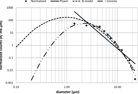
of the matrix has therefore only to be performed once for every instrument setting. Figure 1 illustrates the three models for a randomly selected particle count.

Once the models are calibrated, they can be used to rapidly obtain any desired property of the suspension. To obtain the total number of particles in any random size interval between

d1and d2, using the Ceronio model for illustration:

#d1,d2 = A

d2

Z

d1

dβ·ln d+C·dd (4)

The corresponding total particle volume (assuming the particles to be spheres) in any random size interval between

d1and d2is calculated with:

Vd1,d2=

πA

6

d2

Z

d1

dβ·ln d+C+3·dd (5)

1 0.001 0.01 0.1 1 10 100 1000

0.10 1.00 10.00

n o rm a li sed c o u n ts ( # / m ℓ .µ m ) diameter (µm)

Normalised Power B-model Ceronio

Figure 1.The power law, the variable-βmodel and the Ceronio model, fitted to the same particle count.

The power of the Ceronio model lies predominantly in its ability to model suspensions where the maximum normalised

counts deviate from d=1µm. The diameter where the

nor-malised count reaches a maximum is provided by:

dmax = e−C/2β (6)

3 Model application

3.1 Particle counting data collection

Rand Water is a drinking water supplier supplying about

3.7 million m3/day to a population of roughly 11 million

people in the Gauteng Province, as well as parts of the Mpumalanga, Free State and North West provinces of South Africa. Its primary water source is Vaal Dam, an

impound-ment of 2536 million m3_{. Raw water is conveyed from the}

Vaal Dam by open channel and pipes to two treatment plants – Zuikerbosch (ZB) and Vereeniging (VG). At Zuikerbosch, the bulk of the raw water is first retained in a large balanc-ing tank before it proceeds to treatment; at Vereenigbalanc-ing there is no balancing tank and the water is treated directly upon arrival.

Table 1.Percentage of samples that recorded zero counts in the channels indicated.

Channel dmin dmax ZB ZB VG VG

Raw Final Raw Final

9 10 15 0 % 0 % 0 % 0 %

10 15 20 0 % 0 % 0 % 0 %

11 20 25 6 % 14 % 16 % 9 %

12 25 30 37 % 44 % 46 % 38 %

13 30 40 52 % 46 % 64 % 46 %

14 40 50 87 % 71 % 86 % 78 %

15 50 100 92 % 88 % 93 % 86 %

3.2 Data screening

The particle counter used was a PAMAS 3116 FM with 16

channels, covering the range from 1µm upwards. The

chan-nels used are separated at 1; 2; 3; 4; 5; 6; 7; 8; 10; 15; 20;

25; 30; 40; 50, and 100µm. From these channel boundaries,

the geometric mean of each channel was calculated to obtain the “d” required for the calibration matrices provided earlier.

From the differential counts in each channel, the normalised

counts were calculated by dividing them by the width of each channel, to obtain the “N” in the calibration matrices. The d-and N-values were used for further analysis.

For both the raw and treated water samples, there were very few counts in the higher size ranges. A necessary data screening step was to eliminate those larger channels which returned zero values, therefore not contributing to a meaning-ful fit of the data. The results are shown in Table 1. The chan-nels in the lower half of Table 1 were eliminated from further consideration, based on the large percentage of samples

hav-ing zero particle counts. There were therefore 15−4=11 data

points available for each calibration. After accounting for the

three parameters in the Ceronio model, this left 11−3=8

de-grees of freedom, which is considered adequate for the pur-pose of reliable model calibration. The few zero counts in channel 11 were replaced by values of “1” to prevent the cal-ibration procedure from trying to take the logarithm of zero.

3.3 Comparison of the Ceronio and variable-βmodels

Both the Ceronio and variable-βmodels were calibrated for

each of the 321 samples. The goodness of fit for each sample was determined from the sum of squares SS, i.e. the sum of

the squared differences between the logarithm of the actual

count and logarithm of the modelled count. Figures 2 and 3 show the cumulative distributions for the SS for the Zuiker-bosch and Vereeniging samples respectively. They clearly show the improvement in fit brought about by the Ceronio model. The sums of squares were reduced by 30 to 40 % in all cases, the improvement thus being about the same for both treatment plants, and for both raw and treated water.

1

0% 10% 20% 30% 40% 50% 60% 70% 80% 90% 100%

0.0 0.5 1.0 1.5 2.0 2.5 3.0 3.5 4.0

p

er

ce

n

ta

g

e

sm

a

ll

e

r

th

a

n

sum of squares SS B-model ZB raw SS Ceronio ZB raw

SS B-model ZB Final SS Ceronio ZB Final

Figure 2.Cumulative sum of square for the ZB treatment plant.

1

0% 10% 20% 30% 40% 50% 60% 70% 80% 90% 100%

0.0 0.5 1.0 1.5 2.0 2.5 3.0 3.5 4.0

p

e

rc

en

ta

g

e

sm

a

ll

er

t

h

a

n

sum of squares

SS B-model VG raw SS Ceronio VG raw SS B-model VG Final SS Ceronio VG Final

Figure 3.Cumulative sum of square for the VG treatment plant.

4 Discussion of the Ceronio model

Some of the samples included in Figs. 2 and 3 were not modelled very accurately, as evidenced by their large sum of squares. For this section, where general guidelines for the Ceronio model constants are discussed, the data had to be further screened to include only those samples which could be modelled within a sum of squares of 2. This filtering step removed 56 (17 %) samples from the data set, about evenly spread amongst the four sampling positions, which

left 265 samples (VG Raw: n=65; VG Final: n=67; ZB

Raw: n=69; ZB Final: n=64). The parameter values of

these samples were used to determine the cumulative distri-butions for the four sampling points discussed below.

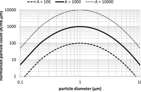
Parameter A determines the height of the size distribution, as shown in Fig. 4. As expected for a surface water impound-ment subject to sharp seasonal turbidity variations, this pa-rameter covers a broad range. The value of A corresponds

directly to the normalised count at d=1µm, similar to its

in-terpretation for the variable-βmodel. From Fig. 5, the raw

water samples had A-values about two orders of magnitude higher than the final treated water samples.

Parameter β, as shown in Fig. 6, determines the

1

1 10 100 1000 10000

0.1 1 10

n

o

rm

a

li

se

d

p

a

rt

ic

le

c

o

u

n

t

(#

/m

ℓ

.μ

m

)

particle diameter (μm)

A = 100 A = 1000 A = 10000

Figure 4.The effect of model parameter A on the particle size dis-tribution, withβ=−1 and C=0.

1

0% 10% 20% 30% 40% 50% 60% 70% 80% 90% 100%

10 100 1000 10000 100000

p

e

rc

e

n

ta

g

e

s

m

a

ll

e

r

th

a

n

parameter A (#/ml.μm)

VG Raw ZB Raw VG Final ZB Final

Figure 5.The cumulative distribution of model parameter A.

Fig. 7 is that the cumulative distributions for the raw and

treated waters are not different. Using the 10th and 90th

per-centiles as guidelines, the range ofβwas from−1.4 to−0.5.

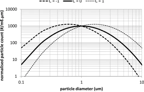
Parameter C moves the size distribution from left to right, as shown in Fig. 8. Figure 9 indicates that the range of C is

between−1.5 to+1.5. The C-values of the raw water samples

lie consistently to the left of the C-value of the treated water samples, indicating that the raw waters had relatively more small particles than the treated water samples. The median

value of dmax for the raw water samples is at 0.8µm (10th

percentile 0.4µm, 90th percentile 1.6µm). Although the

me-dian value of dmaxfor the treated water samples is at 1.0µm

(10th percentile 0.3µm; 90th percentile 1.7µm), its

variabil-ity emphasises the weakness of the variable-βmodel, which

forces dmaxto be 1µm in all cases.

It is pointed out that the dmaxvalues discussed in the

previ-ous paragraph are values predicted from the Ceronio model, and are not directly supported by the particle counting data. The smallest particles that could be counted, due to the tech-nological limitations of the particle counter, are in the

inter-val between 1 and 2µm, which are characterised by a mean

1

1 10 100 1000 10000

0.1 1 10

n

o

rm

a

li

se

d

p

a

rt

ic

le

c

o

u

n

t

(#

/m

ℓ

.μ

m

)

particle diameter (μm)

B = -1.5 B = -1.0 B = -0.5

Figure 6.The effect of model parameterβon the particle size dis-tribution, with A=1000 and C=0.

1

0% 10% 20% 30% 40% 50% 60% 70% 80% 90% 100%

-2.0 -1.5 -1.0 -0.5 0.0

p

e

rc

e

n

ta

g

e

s

m

a

ll

e

r

th

a

n

parameter β

VG Raw ZB Raw VG Final ZB Final

Figure 7.The cumulative distribution of model parameterβ.

particle diameter of 1.4µm. This means that the values for

dmax are mostly just smaller than the smallest particles that

could actually be counted, with no data points to validate the shape and position of the apex of the predicted particle count. This is an unfortunate limitation, which of course

ap-plies equally to the validation of the variable-βand Ceronio

models. This implies that, until this validation can be done by including smaller particles, not too much weight should

be lent to the exact value of dmax. For purposes involving

particle sizes above 2µm, the general conclusions regarding

the Ceronio constants are firmly supported by the data sets used.

5 Summary and conclusions

1

1 10 100 1000 10000

0.1 1 10

n

o

rm

a

li

se

d

p

a

rt

ic

le

c

o

u

n

t

(#

/m

ℓ

.μ

m

)

particle diameter (um) C = -1 C = 0 C = 1

Figure 8.The effect of model parameter C on the particle size dis-tribution, with A=1000 andβ=−1.

amongst particle counting results done with different

in-strument settings.

– Mathematical models present an opportunity to com-press the particle counting data into two or three model parameters, which are much more amenable to analysis and interpretation. Moreover, the models are calibrated using all the channels with non-zero counts, thus pro-viding a more robust description than could be obtained from using single counts from individual channels.

– The power law, commonly used, has two serious short-comings which prohibit its use at both ends of the size spectrum. As the size gets smaller, the number of parti-cles approaches infinity; as the size gets larger, the vol-ume of particles approaches infinity.

– The variable-βmodel removes the shortcomings of the power law, but has its own limitation. Regardless of the sample, the maximum normalised particle count is

al-ways found at a size of 1µm.

– This paper developed an earlier proposal to remove the

limitation of the variable-βmodel, here called the

Cero-nio model. By introducing a third model parameter, the Ceronio model can describe a distribution with the max-imum normalised count at any size.

– Using 321 samples of both raw and treated water from a large South African drinking water supplier, the Cero-nio model consistently provided a better fit than the

variable-β model, reducing the sum-of-squares by

be-tween 30 % and 40 %.

– A systematic analysis of the three parameters describ-ing the Ceronio model provided useful insights. Param-eter A is a paramParam-eter closely related to the number of particles in a sample; parameter B provides a measure of the ratio of smaller to larger particles; and parameter C 1

0% 10% 20% 30% 40% 50% 60% 70% 80% 90% 100%

-2.0 -1.0 0.0 1.0 2.0 3.0

p

e

rc

e

n

ta

g

e

s

m

a

ll

e

r

th

a

n

parameter C

VG Raw ZB Raw VG Final ZB Final

Figure 9.The cumulative distribution of model parameter C.

predominantly influences at which size the maximum normalised particle count is found.

– Potentially, the most important predictions of the Cero-nio model deals with those small particles between

0.1µm and 2µm. This is the size range where the

max-imum normalised particles counts are found, and also where the fundamental transport mechanisms of parti-cles in water are at their weakest. Unfortunately, the

particle counter used could not measure sufficient data

points in this range to provide solid experimental veri-fication of the Ceronio model, indicating an important research need.

– For larger particles, the Ceronio model provides a ro-bust tool for the computation and comparison of par-ticle numbers and volumes at any desired parpar-ticle size interval.

Acknowledgements. The authors express their gratitude to Rand Water for making available the particle counting data and for assistance in the preparation of this paper.

Edited by: J. Verberk

References

Ceronio, A. D. and Haarhoff, J.: An improvement on the power law for the description of particle size distribution in potable water treatment, Water Res., 39, 305–313, 2005.

Lewis, C. M. and Manz, D. H.: Light-scatter particle counting: Improving filtered-water quality, J. Environ. Eng., 117, 15 pp., 1991.

Sheldon, R. W.: Measurement of phytoplankton growth by particle counting, Limnol. Oceanogr., 24, 760–767, 1979.