www.nonlin-processes-geophys.net/15/751/2008/ © Author(s) 2008. This work is distributed under the Creative Commons Attribution 3.0 License.
Nonlinear Processes
in Geophysics
Initial state perturbations in ensemble forecasting
L. Magnusson, E. K¨all´en, and J. Nycander
Department of Meteorology, Stockholm University, 106 91 Stockholm, Sweden
Received: 19 February 2008 – Revised: 3 September 2008 – Accepted: 3 September 2008 – Published: 21 October 2008
Abstract. Due to the chaotic nature of atmospheric dynam-ics, numerical weather prediction systems are sensitive to er-rors in the initial conditions. To estimate the forecast un-certainty, forecast centres produce ensemble forecasts based on perturbed initial conditions. How to optimally perturb the initial conditions remains an open question and different methods are in use. One is the singular vector (SV) method, adapted by ECMWF, and another is the breeding vector (BV) method (previously used by NCEP). In this study we com-pare the two methods with a modified version of breeding vectors in a low-order dynamical system (Lorenz-63). We calculate the Empirical Orthogonal Functions (EOF) of the subspace spanned by the breeding vectors to obtain an or-thogonal set of initial perturbations for the model. We will also use Normal Mode perturbations. Evaluating the results, we focus on the fastest growth of a perturbation. The re-sults show a large improvement for the BV-EOF perturba-tions compared to the non-orthogonalised BV. The BV-EOF technique also shows a larger perturbation growth than the SVs of this system, except for short time-scales. The highest growth rate is found for the second BV-EOF for the long-time scale. The differences between orthogonal and non-orthogonal breeding vectors are also investigated using the ECMWF IFS-model. These results confirm the results from the Loernz-63 model regarding the dependency on orthogo-nalisation.
1 Introduction
Both initial state errors and model errors are undesirable but inevitable features of any numerical weather prediction sys-tem. To estimate the error growth, forecast centres produce ensemble forecasts. An ensemble forecast is composed of a number of simulations (ensemble members), with differ-ent initial states and/or model formulations. The differences
Correspondence to: L. Magnusson ([email protected])
in initial states and model formulations are designed to es-timate the respective uncertainties. For the initial-state per-turbations, several characteristics are desirable. One of them is that the perturbations are realistic in the sense that they represent possible atmospheric perturbations consistent with uncertainties in the observed properties of the atmosphere. Another desirable feature is to capture the fastest growing modes out of these that are both realistic and compatible with the uncertainty. Perturbation growth will be the focus for this study.
The initial error growth is approximately exponential but as the error grows the growth rate declines, and after about two weeks the error saturates. Both error saturation and the chaotic dynamics of the atmosphere can be associated with the nonlinear nature of the equations governing atmo-spheric dynamics. In this study we will compare several techniques that can be used to construct initial state pertur-bations. The methods will be applied to a simplified model (Lorenz, 1963) that has error growth characteristics similar to those of the real atmosphere. The properties found in the simplified Lorenz-63 are used to design experiments with a comprehensive weather prediction system, the ECMWF IFS-model.
A purely stochastic perturbation is very likely to decrease in time as most phase space directions in atmospheric models will produce gravity-wave-like motion that will die out rather quickly in a forecast integration. Other types of perturbations that grow quickly on a time scale of a few days may instead be associated with particular model balances that only rarely, if ever, are observed. Perturbing a forecast model in this way will result in rapidly growing perturbations but the resulting error growth may not properly represent the real uncertainty of the observations.
model dynamics to generate perturbations while the singular vector method utilises a mathematical technique that opti-mises perturbation growth over a given time interval. Pertur-bations constructed by the singular vector method could give rise to structures rarely observed in the atmosphere (Isaksen et al., 2005).
In this study we will focus on the growth of small initial-state differences in a very simple model. The model used is the Lorenz-63 model (Lorenz, 1963). Numerous studies have been made using this system during the past decades, e.g. Smith et al. (1999), Palmer (1993) and Anderson (1996). In Palmer (1993) the predictability of the Lorenz-63 model is investigated, and it is found that the predictability differs significantly between different parts on the attractor. In An-derson (1996) different ensemble methods are compared on the Lorenz-63 model.
When there is more than one perturbed forecast, the or-thogonality of the perturbations is important for finding the fastest growing perturbations, especially in a low-order sys-tem. For breeding vectors this is discussed by Annan (2004). He found that by using 2 orthogonal breeding vectors it was possible to capture the fastest-growing perturbations more ef-fectively. We will extend his study and use orthogonal BV to see how effectively the fastest growing modes are captured compared to singular vectors. In the present study we use the empirical orthogonal functions (EOF) of a set of breeding vectors as initial perturbations.
The BV-EOF and singular vector methods are compared with random perturbations and also other constrained meth-ods (normal mode and the original, non-orthogonalised, breeding method). Here, the definition of a constrained method is that it only samples some subspace of the complete model phase space (Anderson, 1997). The growth of per-turbations generated by the different methods is compared. In addition to the Lorenz-63 model, we use the numerical weather prediction model used by ECMWF, to further in-vestigate some properties found in the simple system. Some fundamental conclusions concerning the methods are made which are believed to be of relevance for full-scale NWP sys-tems.
2 The Lorenz-63 model
The chaotic model used here, first introduced by Lorenz (1963), is a simplified model based on convective dynam-ics, and has been widely used in chaos research. The model equations are:
˙
x=σ (y−x), (1)
˙
y=rx−y−xz, (2)
˙
z=xy−bz. (3)
The system is 3-dimensional, non-linear and has a chaotic behaviour for the widely used parameter valuesσ=10,r=28 andb=8/3 (also used in this paper). The attractor of the
system is a quasi-2-dimensional (fractal dimension about 2.05) structure with the famous “butterfly-wings” shape. (Al-though the dimension >2 it consists of fairly well-defined planes in the “wings”.) The system has 3 fixed points. The origin is a saddle point with one strongly unstable direction. The centres of the wings are weakly unstable spirals in the attractor plane and stable in the direction orthogonal to the attractor plane. Two time-scales appear in the system. One describes the rotation around the centre of a wing and the second the residence time within one of the butterfly wings (Palmer, 1993). The short time scale is around 0.75 time unit (tu). The long time scale is influenced by the chaotic behaviour of the system and can be defined in a statistical sense. It is around 1.8 tu.
The system of Eqs. (1–3) can be formulated as
˙
x=F (x). (4)
The growth of a perturbation (1x=x−x0) can be studied by linearisation of the system around a point at timet:
1x˙ =F(x(t ))−F(x0(t ))∼=J(t )·1x, (5) where
J(t )=∂F
∂x|x=x0(t ). (6) The eigenvalues of the Jacobian J in Eq. (6) gives infor-mation about the evolution of the perturbations. If the real part of an eigenvalue is positive (negative), the perturbation is growing (decreasing) in the direction of the corresponding eigenvector. Because of the dimensionality of the system,
J has the three eigenvalues (in arbitrary order)e1=a1+ib1, e2=a2+ib2,e3=a3+ib3. Even though the system is chaotic, the real parts of all three eigenvalues are negative in some points (an<0 for alln). As the Lorenz-63 system is
dissi-pative,a1+a2+a3<0 for all points (Lorenz, 1963). The dif-ferences in growth rate of perturbations differs widely as a function of location on the attractor as illustrated in Fig. 3 in Evans et al. (2004). Especially in the intersection of the butterfly wings the perturbation growth rate is high.
3 Constrained methods
The aim of this study is to find the perturbation that best approximates the local, fastest growing mode. The eigen-value structure and its changes along the attractor trajecto-ries are important for the constrained perturbations, but in different ways. The normal mode perturbations are directly constructed from the eigenvalue structure in the initialisation point. Breeding vectors use the dynamics from the previous simulation and are therefore sensitive to changes in the eigen-value structure (the dynamics of the system) preceding the new initialisation of the ensemble. Singular vectors use the
3.1 Normal modes (NM)
The normal-mode method identifies the fastest growing eigenmode for the initial point by (as discussed in Sect. 2) using the eigenvalues of the Jacobian of the system:
Jv=λv. (7)
By calculating the eigenvector for the largest positive eigen-value, the direction of the fastest growing eigenmode of the instantaneous Jacobian is found.
If the dominating eigenvalue is complex the fastest grow-ing eigenmode lies in a plane spanned by vectors constructed by the real part and the imaginary part of the conjugated eigenvectors (equivalent with the plane spanned by the 2 complex-conjugate eigenvectors). In this case we randomise the perturbations in that plane.
3.2 Singular vectors (SV)
To calculate the relative growth of a perturbation, the ratio between the amplitudes of the initial and the final perturba-tion can be calculated:
α= h1x(t ), 1x(t )i h1x(t0), 1x(t0)i
. (8)
wereh,i defines the inner product. If the linear evolution of the system is written in the form1x(t )=M(t, t0)1x(t0), Eq. (8) can be written as
α= hM(t, t0)1x(t0),M(t, t0)1x(t0)i h1x(t0), 1x(t0)i
= 1x
TMTM1x
1xT1x . (9)
Given a norm and optimisation timetthe problem of finding the spatial directions of fastest growing modes can be solved by determining the eigenvalues and eigenvectors ofMTM. These are the singular values and the singular vectors of the system (Palmer, 1999). The propagatorM(t, t0), referred to as the tangent linear model (TLM), is determined by using a basic, unperturbed, trajectory of the system. Therefore the singular vector method is limited to sufficiently small per-turbations. If the perturbations grow larger the evolution of the perturbations determined by the TLM and the non-linear model will differ (Mu et al., 2003). The first approach to the singular vector method comes from Lorenz (1965). The method is described by e.g. Palmer (1993) and used opera-tionally at ECMWF.
3.3 Breeding vectors (BV)
Another method used in NWP is the breeding method (Toth and Kalnay, 1993, 1997). The method was used opera-tionally at NCEP until May 2006. The difference between a perturbed and the unperturbed simulation is re-scaled to a small amplitude at certain times during the integration and added to a new analysis. By starting with different initial conditions additional breeding vectors can be constructed.
From the beginning the initial perturbations are randomly chosen (but as a difference between two realistic atmospheric states), but after a few cycles the breeding vectors converge to the dominant Lyapunov vector, especially in a low order system as Lorenz-63. Hence, the different breeding vectors tend to become linearly dependent.
3.4 BV-EOF
To avoid the problem that breeding vectors are linearly de-pendent, computations of an orthogonal complement to the dominant Lyapunov vector is needed. In for example Ander-son (1996) and Annan (2004) this is done by a Gram-Schmidt orthogonalisation method. In this paper we will use another, more generalizable, method where the orthogonal comple-ment is given by the EOF of the breeding vectors.
Define a matrix whose columns are the breeding vectors, B=[x1−xc,x2−xc, ...,xk−xc] , (10)
wherexi is the state vector for the i-th perturbed forecast of
a k-member ensemble forecast andxcis the state vector for
the unperturbed forecast. The covariance matrix is formed as BTB. The eigenvectors of BTB are the Empirical Orthogonal Functions (EOFs) of the local breeding vector subspace, and the eigenvalues describe the variance in the direction of the EOFs. We will use the EOFs of the covariance matrix as the new ensemble perturbations, by normalising the EOFs with the square root of the corresponding eigenvalue (variance), yielding equal initial amplitude for all EOFs. These are here-after added to the unperturbed forecast. This method will be referred to as BV-EOF in this study. The method scales up additional growing modes in the system, which can be in an early stage of their development.
Operationally, a similar orthogonalisation technique as BV-EOF is used for Ensemble Transform Kalman Filter (Wang and Bishop, 2003). But in the literature the focus has been on the norms used (observation space for ETKF) for the normalisation and not on the properties of the orthogonalisa-tion. Since May 2006 NCEP uses a transformation (ET) of breeding vectors (Wei et al., 2008) as initial perturbations for their ensemble forecasting system. The method is similar to ETKF but yields an orthogonal set of initial perturbations in the inverse analysis error variance norm. The properties we will find regarding othogonality of the BV-EOF technique apply to the ET method as well as ETKF unless the simplex transformation (Wang et al., 2004) for centering the ensem-ble around the analysis is used.
3.5 Norm dependence
linearly dependent ensemble members, as will be seen below. However, the norm dependence of SV and BV-EOF can also be considered as a weakness, since it introduces an arbitrary element in their definition.
In the ECMWF ensemble prediction system an energy norm is used, mainly for practical reasons. Barkmeijer et al. (1999) propose using the Hessian of the cost function (the inverse of the analysis error covariance matrix) to define a norm for the initial perturbation (i.e. the denominator in Eq. 8) that reflects the actual uncertainty. A recent compar-ison (Lawrence et al., 2007) between energy norm and the Hessian norm for singular vector calculations indicates that they generate similar singular vectors.
The norm dependence of the singular vectors has also re-cently been discussed by Kuang (2004).
Notice that it is necessary to define a norm in order to mea-sure the magnitude of the perturbation (or the error) when evaluating the performance of an ensemble, even if no norm is used when constructing the ensemble members. For the Lorenz-63 model we will simply use the Euclidean norm, both when evaluating the ensembles and when constructing the SV and BV-EOF ensembles. The perturbation size for the ECMWF NWP-model results is measured using the total energy norm (Magnusson et al., 2008).
4 Initialisation
We create ensemble members by different methods, both unconstrained (Random Perturbations, RP) and constrained (NM, SV, BV and BV-EOF) in order to compare them. All perturbations initially have the same scalar distance from the unperturbed forecast (centre member). The norm used to cal-culate the differences between the simulations is
||x|| = hx,xi12 =
q
x12+x22+x32. (11) The reason why a simple isotropic norm is used is that the aim of the present study is to find the direction for the fastest growing perturbation of the system, not to sample an error distribution.
The random perturbations are randomly distributed on a spherical shell around the centre member with no preferred directions.
For the SV-method the first two singular vectors are used as perturbations, and for the BV-EOF the two first EOFs. It is a disadvantage of this study that two directions in a 3-dimensional system are used but this is needed to study the improvements obtained through the orthogonalisation. An ordinary (not orthogonal) breeding system (BV) is also used to make it possible to measure the impact of the orthogonali-sation. The cycles for BV and BV-EOF are started from two random perturbations for the very first step.
Perturbations are also made using the normal mode method (NM) whereby the eigenvectors and eigenvalues of
J are calculated and the eigenvector corresponding to the largest eigenvalue is used as a perturbation. In the case when these are complex-conjugate, the perturbation is placed ran-domly in the circle spanned by the real and imaginary part of the eigenvector. This circle is a cross-section of the spherical shell used for the random perturbations.
For time stepping of the Lorenz-63 model we use Heun’s numerical method (Kalnay, 2003). The time step used is 0.01 tu. To let the first initial point of the study be located on the attractor, the model is integrated 3000 steps before the en-semble is initiated. The initial state for each enen-semble mem-ber is determined using the different perturbation methods described above. The length of the perturbation is prescribed as 0.01 length units, which is around 0.05% of the size of the attractor. The choice of the perturbation length is made following the conclusions from Trevisan (1993).
The system is integrated forward in time for each initial state. After a given time interval, the system is restarted with new perturbations for the new initial point. Previous studies have used different restarting intervals, e.g. Annan (2004) used 0.1 tu and Anderson (1997) 1 tu. In our study we use both 0.1 tu and 1 tu as intervals (cycle length) for the rescal-ing, to study how the behaviour of the perturbation depends on the integration length. Those time scales can be compared with the time for the error to saturate on the attractor, which is around 6 tu (Trevisan, 1993). As mentioned above the ro-tation period in a wing is around 0.75 tu and the residence time within one of the attractor wings around 1.8 tu. Because the long time-scale is of the same order as the residence time, it is likely that the trajectories pass locations on the attractor with large perturbation growth rate during the long restart in-terval. We believe that this in practice limits the time interval during which the TLM is valid in the SV calculation.
In our study we focus on perturbation growth. We are not studying the behaviour of the ensemble in terms of skill scores. Therefore we are not using a centred ensemble and no attempt is made to simulate an analysis error. We thus differ from Anderson (1997) who, to simulate the analysis error, also moves the centre of the ensemble away from a “true point” that simulates the actual atmospheric trajectory. This disturbance is made at random, thus moving the initial state away from the attractor of the system. We instead fol-low the trajectory on the attractor, thus assuming that each analysis coincides with the simulated “true state”. The re-sults are however relevant to the analysis error problem as they show which characteristic structures that grow quickest.
5 Results
5.1 Perturbation evolution
0.5 0.6 0.7 0.8 0.9 1 1.1 10−3
10−2 10−1
time
Perturbation size
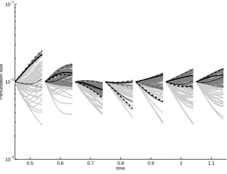
Fig. 1. Evolution of the difference between the central member
and perturbed members, for 7 equally spread initial points taken along a trajectory. Rescaled every 0.1 tu. BV (black, dashed), RP (light-grey, solid),NM (grey, solid), first SV (dark-grey, thick dash-dotted), second SV (dark-grey, thin dash-dotted), first BV-EOF (black, thick solid), second BV-BV-EOF(black, thin solid).
BV and BV-EPS are plotted and simulations of 50 random perturbations. For NM 50 perturbations are plotted if the initial point yields a non-zero imaginary part of the largest eigenvalue, otherwise 1 perturbation is plotted. Note that the difference is plotted on a logarithmic scale.
Figure 1 shows 7 cycles with short restart intervals (0.1 tu). This is an example of a trajectory first passing close to the origin of the attractor, going out in the end of a wing and fi-nally falling into the centre of the other wing. First looking at the unconstrained method (RP), we see that the difference between the central and the perturbed simulation, in many cases, rapidly decreases. This occurs in cases when the ini-tial perturbation has a large component away from the attrac-tor. But the RP also gives us information about the largest possible perturbation growth. E.g. between 0.75 and 0.85 tu the system is stable and it is impossible to find a growing direction.
As mentioned in Sect. 4 the NM perturbations are depen-dent on the eigenvalue structure. For cycle 1 and 4 there is one leading direction, and only one member is used. For the other cycles, the leading direction is confined to a plane and then 50 perturbations are used on that plane. The NM method shows a large improvement compared to RP, espe-cially when the NM perturbations are distributed on a plane. This improvement indicates that using the information about the leading eigenvectors is a useful method for creating per-turbations located close to the attractor of the system.
For the SV method, the first SV is optimised to find the fastest growing direction for the optimisation time. We see that the method performs perfectly in all the cycles.
4 5 6 7 8 9 10 11 12
10−4 10−3 10−2 10−1 100
time
Perturbation size
Fig. 2. Same as Fig. 1 but rescaled every 1 tu.
Figure 2 shows the same kind of plot as above but for a longer time scale. The most obvious result is that the second BV-EOF performs best in almost all the cycles shown here. For the SV method the second SV seems to perform as well as the first, which indicates that the time scale is too long to make the approximation using TLM valid. The breed-ing method is unable to find the fastest growbreed-ing direction of the system. One explanation is that both breeding vectors have become linearly dependent so that only one direction in phase space is spanned.
5.2 Perturbation growth rate
In order to obtain reliable statistics of the perturbation growth, we have run 5000 simulations and calculated the per-turbation growth.
For a chaotic system with exponential perturbation growth rate, the perturbation size at timet+1tis
||1x(t+1t )|| = ||1x(t )||exp(λ1t ) (12)
The instantaneous exponential growth rate (the slope of the curves in Figs. 1 and 2) can be calculated as:
λ= 1
1t ln ||
1x(t+1t )|| ||1x(t )||
(13)
and letting1tgo to zero. The instantaneous growth rate can vary significantly for different parts of the attractor as seen in the previous figures and also discussed in e.g. Palmer (1993). By instead letting1t in Eq. (13) go to infinity and letting 1x(t )go to zero the dominant Lyapunov exponent can be calculated. If the dominant Lyapunov exponent is greater than zero, the system is chaotic (Strogatz, 2000).
0 0.1 0.2 0.3 0.4 0.5 0.6 0.7 0.8 0.9 1 −5
−4 −3 −2 −1 0 1 2 3 4 5
t
exponential growth rate
Fig. 3. Perturbation growth rate in terms of the instantaneous growth rate as an average over 5000 cases. Breeding cycle length and singular vector optimisation time 0.1 tu but the ensembles are run until 1 tu. BV (black, dashed), RP (grey, solid),NM (dark-grey, solid), first SV (black, thick dash-dotted), second SV (black, thin dash-dotted), first BV-EOF (black, thick solid), second BV-EOF (black, thin solid).
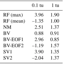
Table 1. Mean exponential growth rate as a mean for 5000
simula-tions for the short (0.1 tu) and long (1 tu) time scale respectively.
0.1 tu 1 tu
RF (max) 3.96 1.90
RF (mean) –1.35 1.00
NM 2.51 1.37
BV 0.88 0.91
BV-EOF1 2.96 0.85
BV-EOF2 –1.19 1.57
SV1 3.90 1.35
SV2 –2.04 1.37
We will use Eq. (13) and letting1t=0.1 tu and1t=1 tu re-spectively as a measure of the mean exponential growth rate using 5000 simulations. In addition to the mean exponential growth for each perturbation method, we have also calcu-lated a maximized growth for the RP method by finding the perturbation yielding the highest exponential growth rate for each simulation. The average of the exponential growth rate for both the short (0.1 tu) and long time scale (1 tu) of each method is shown in Table 1.
Inspired by Fig. 2 in Trevisan (1993), the instantaneous exponential growth rate (letting t in Eq. (13) be the previ-ous time step and1tequal the time step) of all perturbation methods is plotted as a function of time in Figs. 3–4. The results are a mean of 5000 cycles. In Fig. 3 the singular vec-tors are optimised for 0.1 tu (short time-scale) and in Fig. 4
0 0.1 0.2 0.3 0.4 0.5 0.6 0.7 0.8 0.9 1
−5 −4 −3 −2 −1 0 1 2 3
t
exponential growth rate
Fig. 4. Same as Fig. 1 but breeding cycle length and singular vector
optimasation time 1 tu. The NM and RP simulations are the same as in Fig. 3.
for 1 tu (long time-scale). The same values are used for the breeding cycle length in the figures respectively. All simula-tions are made until 1 tu, which implies that the simulasimula-tions for BV and BV-EOF is run until 1 tu even if the perturbations are calculated using a cycle length of 0.1 tu.
For the breeding method (black, dashed), we see that the exponential perturbation growth is constant in time. The av-erage exponent is 0.88 for the short time-scale and 0.91 for the long. These values agree well with the value of the dom-inant Lyapunov exponent for the Lorenz-63 in the literature (0.90).
For the random perturbations (grey, solid), the perturba-tions generally decrease initially while the perturbaperturba-tions ap-proach the attractor. But after about 0.1 tu the perturbation growth increases and shows a period with growth rate faster than the Lyapunov exponent, referred as transient growth in Trevisan (1993). After that stage, the growth converges to-wards the dominant Lyapunov exponent. The average ex-ponential growth calculated using Eq. (13) from t=0 and 1t=0.1 for the short scale is –1.35. For the long time-scale (t=1) the value is 1.00, which is higher than the one for BV. This shows that on a long time scale it is possible to obtain growing perturbations using random perturbations.
to detect the maximum and minimum possible perturbation growth, all tests was also run using 10 000 random perturba-tions. The values for using 10 000 simulations were then 3.96 and –15.4 (0.1 tu), respectively, and 1.91 and –4.07 (1 tu). This indicates that results obtained by 1000 perturbations are robust at least for the maximum perturbation growth.
For the normal mode perturbations (dark-grey, solid), we see that the perturbations have an exponential growth rate larger than the dominant Lyapunov exponent from the begin-ning. The growth rate reaches a maximum at 0.1 tu. The mean growth rate for the short time-scale is 2.51. Then the growth rate decreases and approaches the dominant Lya-punov exponent. The average exponent for normal mode for the long time-scale is 1.37. The immediate growth of the NM perturbations is a clear sign that the method finds the attrac-tor of the system. The NM perturbation shows a period of transient perturbation growth until 0.5 tu. After that period a perturbation growth smaller than the Lyapunov exponent appears as expected after a period of transient growth.
The first singular vector using optimisation time 0.1 tu (Fig. 3, black, thick dash-dotted) shows the fastest perturba-tion growth with an average of 3.90, very close to the max-imum possible growth rate. This indicates, as mentioned above, that the TLM is a good approximation of the non-linear system for this time-scale. Regarding the longer time scale, using optimisation time 1 tu (Fig. 4), the growth rate for the first SV is 1.35, significantly lower than the maxi-mum value 1.90 for the system (and also lower than the NM value). This indicates that the perturbation during the long time scale reached an amplitude so that the TLM and the non-linear model will diverge.
Studying BV-EOF for the short time scale, using breed-ing cycle length 0.1 tu, the first BV-EOF (black, thick solid) grows at a much higher growth rate than the non-orthogonal breeding vectors and the average exponent is 2.96. The second BV-EOF shows decreasing perturbations (negative growth rate) in the mean. But for the longer time scale, the highest perturbation growth is found for the second BV-EOF (1.57), using breeding cycle length 1 tu. This is remarkable, both regarding the superiority to SV and especially that the second EOF grows faster than the first one. The growth for the first BV-EOF is very similar to the BV (and the dominant Lyapunov exponent). This because both the BV-EOF per-turbations converge to the dominant Lyapunov vector dur-ing the breeddur-ing cycle usdur-ing the long time-scale, implydur-ing that the first BV-EOF will be similar to that direction. The higher perturbation growth rate for the second EOF perturba-tion could be related to non-orthogonal eigenvectors as dis-cussed in Smith et al. (1999). Because of this the second BV-EOF could have a finite time of transient perturbation growth as seen in Fig. 4, before converging to the leading Lyapunov direction.
In order to investigate if it is possible to optimise the per-turbation growth for SV and the breeding methods for the long time scale, the optimisation time and breeding cycle
length were changed with the evaluation time kept fixt at 1 tu. Changing optimisation time for SV means that we optimise the perturbation growth for perturbation amplitudes were the TLM approximation is valid and hope that the perturbations continue growing also for later time steps (when reaching the non-linear regime). Highest perturbation growth, regarding the long time scale, is found to be 1.56, using optimisation time 0.15 tu.
For the breeding perturbations, the highest perturbation growth was found for breeding cycle length 1 tu (1.57 for the second BV-EOF). Using a short cycle length (0.05 tu) the first BV-EOF achieves a higher growth rate (1.39) than the second (0.98).
To test the sensitivity to the initial perturbation length, simulations where also made with the length 0.1 and 0.001 for 1 tu. The results are in line with the results for simulations using 0.01 indicating that also small initial perturbations will reach the limit for the TLM approximation during 1 tu. This indicates that the important factor for the validity of the ap-proximation is not the perturbation size but the time-scales of the dynamical system (i.e. how long time it takes for the system to reach a location with large perturbation growth).
6 Breeding experiments using ECMWF NWP-model
To investigate the properties of orthogonal breeding vectors regarding perturbation growth in a more realistic environ-ment, we have used the ECMWF IFS-model with spectral resolution TL95 and 40 vertical levels. The BV and
BV-EOF methods are implemented as described in Sect. 3 and for the orthonormalisation a total energy norm is used. We have used a breeding cycle length of 6 h and we have run 30 simulations with 10 ensemble members. For further details about the non-orthogonal breeding experiment see Magnus-son et al. (2008) (simple breeding).
0 5 10 15 20 25 −4
−2 0 2 4 6 8 10 12 14
Perturbation amplification
Member number
Amplification rate (%)
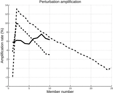
Fig. 5. Perturbation amplification as function of perturbation
num-ber using ECMWF IFS-model for 10 breeding vectors (solid), BV-EOF with ensemble size 10 members (dashed) and 25 members (dash-dotted).
In addition to the two experiments described above we have run a BV-EOF ensemble with 25 members (dash-dotted). The results show a low amplification rate for the first member, in fact even a decrease of the perturbation am-plitude. For the following members we see an increased per-turbation growth rate compared to the 10 member ensem-ble. Taking a mean of the perturbation amplification we ob-tain 5.2%, a lower value compared to the breeding experi-ment. By instead calculating the perturbation amplification for members 2 to 11 we obtain 9.7%, a clear difference to the non-orthogonal breeding experiment and the 10-member BV-EOF ensemble. For ensemble forecasting, it could there-fore be possible to obtain higher ensemble dispersion by run-ning several breeding cycles but only use a subset of the members for the ensemble and exclude member number one. One explanation (as discussed in the previous section) is that the BV-EOF perturbations (except the first) undergo a pe-riod with transient perturbation growth. But this does not explain why the first BV-EOF has a growth rate much lower than the breeding vectors. Another explanation of the de-cline of ensemble member number one could be the time his-tory of structures used to generate BV-EOF ensembles. The structures with most variance may contain modes that have reached a mature stage of development and have started to decline. If such mature structures dominate ensemble mem-ber nummem-ber one we should thus expect to see a declining am-plitude.
7 Summary and conclusions
In this study we have compared different initial perturba-tions strategies to find the direction with highest perturbation growth in the simple Lorenz-63 system. For the study, we have used two time scales.
Studying the short time scale, it was found that the pertur-bations generally must lie within the attractor subspace of the phase space. If this is not the case, the perturbed trajectory will in many cases quickly approach the unperturbed, cen-tral forecast trajectory. This is demonstrated in the present study by the fact that unconstrained perturbations rapidly de-cay most during the first time steps. If the perturbation is confined to the attractor it starts to develop at a higher pace. Studying a longer time scale, this constraint is not so strong; the random perturbations originally outside the attractor start to grow after reaching the attractor.
By studying the eigenvectors of the linearized model around the initial point some important information on the phase space directions giving large growth rates can be found. A perturbation made from this information (NM) shows large growth rate, especially for the short time scale. We conclude that the NM method usually succeeds in con-fining the perturbations to the attractor.
For the short restart interval, the singular vector method finds the fastest growing direction perfectly. But for a longer time scale this is not the case. Since the singular vectors are found by optimising the growth of the tangent linear model, the fact that BV-EOF is superior to SV for the long time scale must be an effect of the approximations using the tangent lin-ear model. To optimise the perturbation growth for a longer time scale it should be possible to use conditional non-linear optimal perturbations, CNOP (Mu et al., 2003). CNOP finds the most unstable perturbations by maximising the perturba-tion using the non-linear model instead of the tangent linear model. The result should be equal to the random perturba-tion with maximal amplificaperturba-tion, if the set of RP fills the shell around the unperturbed point (which is possible in a three-dimensional system using 1000 perturbations but not in a NWP-model).
We found that it is possible to obtain a higher perturbation growth for SV on a long time scale by shortening the optimi-sation time. This method is used in the operational singular vector system at ECMWF were the optimisation time is set to 48 h even if the focus for the ensemble forecast is in the medium range (3–8 days).
Therefore it can be seen as an advantage for the BV-EOF that the perturbations inherit this property.
To further investigate the differences between orthogonal and non-orthogonal breeding vectors, experiments were un-dertaken using the ECMWF IFS-model. The results confirm that higher perturbation growths in individual members were obtained by using orthogonal breeding vectors. The pertur-bation growth rate decreases with the perturpertur-bation number. In the NWP model as in the simple model, the first EOF yields a low growth rate. However, the physical reason for this property needs further investigation.
The results for the perturbation growth dependence of EOF number have implications for operational weather fore-casting systems. Using Ensemble Transform Kalman Filter techniques when constructing perturbations should show the same properties as the BV-EOF regarding the ordering. By using a subspace of the total ensemble members, a more ef-fective ensemble in terms of perturbation growth could be obtained.
The conclusion is that the BV-EOF method has the advan-tage with respect to the non-orthogonal breeding method by choosing the directions that grow fastest locally but also has the advantage with respect to SVs that the perturbations are confined within in the subspace of the Lyapunov vectors.
Another conclusion, obtained by the both the normal mode method and BV-EOF, and applicable to operational forecast-ing systems is that perturbations located on the attractor will start to grow with a reasonable pace. Therefore it should be possible to construct an ensemble using information about the observed atmospheric variability, which can be found in comprehensive atmospheric databases such as reanalyses (ERA-40, NCEP) or an operational forecasting archive. Us-ing such a database to construct the perturbations we are more likely to confine them within the atmospheric attractor.
Acknowledgements. We acknowledge Anna Trevisan and one
anonymous reviewer for valuable comments during the preparation of this paper.
Edited by: O. Talagrand
Reviewed by: A. Trevisan and another anonymous referee
References
Anderson, J. L.: Selection of Initial Conditions for Ensemble Fore-casts in a Simple Perfect Model Framework, J. Atm. Sci, 53, 22–36, 1996.
Anderson, J. L.: The Impact of Dynamical Constraints on the Selec-tion of Initial CondiSelec-tions for Ensemble PredicSelec-tions: Low-Order Perfect Model Results, Mon. Weather Rev., 125, 2969–2983, 1997.
Annan, J. D.: On the Orthogonality of Bred Vectors, Mon. Weather Rev., 132, 843–849, 2004.
Barkmeijer, J., Buizza, R., and Palmer, T. N.: 3D-Var Hessian sin-gular vectors and their potential use in ECMWF Ensemble Pre-diction System, Q. J. Roy. Met. Soc., 125, 2333–2351, 1999. Evans, E., Bhatti, N., Kinney, J., Pann, L. Pe˜na, M., Kalnay, E., and
Hansen, J.: Undergraduates find that regime changes in Lorenz’s model are predictable, BAMS, 85, 520–524, 2004.
Farrell, B. F.: Small Error Dynamics and the Predictability of At-mospheric Flows, J. Atm. Sci., 47, 2409–2416, 1990.
Isaksen, L., Fisher, M., Andersson, E., and Barkmeijer, J.: The structure and realism of sensitivity perturbations and their inter-pretation as “Key Analysis Errors”, Q. J. Roy. Met. Soc., 131, 2053–3078, 2005.
Kalnay, E.: Atmospheric Modeling, Data Assimilation and Pre-dictability, p. 83, Cambridge University Press, 2003.
Kuang, Z.: The Norm Dependence of Singular Vectors, J. Atm. Sci., 61, 2943–2949, 2004.
Lawrence, A. R., Leutbecher, M., and Palmer, T. N.: Comparison of Total Energy and Hessian Singular Vectors: Implications for Observation Targeting, Q. J. Roy. Met. Soc., submitted , 2008. Lorenz, E. N.: Deterministic Nonperiodic Flow, J. Atm. Sci., 20,
130–141, 1963.
Lorenz, E. N.: A study of the predictability of a 28-variable atmo-spheric model, Tellus, 67, 321–333, 1965.
Magnusson, L., Leutbecher, M., and K¨all´en, E.: Comparison be-tween Singular Vectors and Breeding Vectors as Initial Pertur-bations of ECMWF Ensemble Prediction System, Mon. Weather Rev., 136, 4092–4104, 2008.
Mu, M., Duan, W. S., and Wang, B.: Conditional nonlinear optimal perturbation and its applications, Nonlin. Processes Geophys., 10, 493–501, 2003,
http://www.nonlin-processes-geophys.net/10/493/2003/. Palmer, T. N.: Extended-Range Atmospheric Prediction and the
Lorenz Model, Bull. Am. Meteor. Soc., 74, 49–66, 1993. Palmer, T. N.: Predicting uncertainty in forecasts of weather and
climate, Technical Memorandum 294, ECMWF, 1999.
Smith, L. A., Ziehmann, C., and Fraedrich, K.: Uncertainty dynam-ics and predictability in chaotic systems, Q. J. Roy. Met. Soc., 125, 2855–2886, 1999.
Strogatz, S. H.: Nonlinear dynamics and choas, p. 497, Westview Press, 2000.
Toth, Z. and Kalnay, E.: Ensemble Forecasting at NCEP: The Gen-eration of Perturbation, Bull. Am. Meteor. Soc., 74, 2317–2330, 1993.
Toth, Z. and Kalnay, E.: Ensemble Forecasting at NCEP and the Breeding Method, Mon. Weather Rev., 125, 3297–3319, 1997. Trevisan, A.: Impact of Transient Error Growth on Global Average
Predictability Measures, J. Atm. Sci., 50, 1016–1028, 1993. Wang, X. and Bishop, C.: A Comparison of Breeding and Ensemble
Transform Kalman Filter Ensemble Forecast Schemes, J. Atm. Sci., 60, 1140–1158, 2003.
Wang, X., Bishop, C., and Julier, S.: Which Is Better, an Ensem-ble of Positive-Negative Pairs or a Centered Spherical Simplex Ensemble?, Mon. Weather Rev., 132, 1590–1605, 2004. Wei, M., Toth, Z., Wobus, R., and Zhu, Y.: Initial Perturbations