www.atmos-meas-tech.net/9/4487/2016/ doi:10.5194/amt-9-4487-2016
© Author(s) 2016. CC Attribution 3.0 License.
High-spatial-resolution mapping of precipitable water vapour using
SAR interferograms, GPS observations and ERA-Interim reanalysis
Wei Tang1, Mingsheng Liao1,2, Lu Zhang1, Wei Li3, and Weimin Yu4
1State Key Laboratory of Information Engineering in Surveying, Mapping and Remote Sensing,
Wuhan University, Wuhan, China
2Collaborative Innovation Center for Geospatial Technology, Wuhan University, Wuhan, China 3Shanghai Academy of Spaceflight Technology, Shanghai, China
4Shanghai Institute of Satellite Engineering, Shanghai, China
Correspondence to:Lu Zhang ([email protected])
Received: 13 December 2015 – Published in Atmos. Meas. Tech. Discuss.: 27 January 2016 Revised: 15 June 2016 – Accepted: 25 August 2016 – Published: 12 September 2016
Abstract.A high spatial and temporal resolution of the pre-cipitable water vapour (PWV) in the atmosphere is a key requirement for the short-scale weather forecasting and cli-mate research. The aim of this work is to derive tempo-rally differenced maps of the spatial distribution of PWV by analysing the tropospheric delay “noise” in interferomet-ric synthetic aperture radar (InSAR). Time series maps of differential PWV were obtained by processing a set of EN-VISAT ASAR (Advanced Synthetic Aperture Radar) images covering the area of southern California, USA from 6 Oc-tober 2007 to 29 November 2008. To get a more accurate PWV, the component of hydrostatic delay was calculated and subtracted by using ERA-Interim reanalysis products. In ad-dition, the ERA-Interim was used to compute the conver-sion factors required to convert the zenith wet delay to wa-ter vapour. The InSAR-derived differential PWV maps were calibrated by means of the GPS PWV measurements over the study area. We validated our results against the measure-ments of PWV derived from the Medium Resolution Imag-ing Spectrometer (MERIS) which was located together with the ASAR sensor on board the ENVISAT satellite. Our com-parative results show strong spatial correlations between the two data sets. The difference maps have Gaussian distribu-tions with mean values close to zero and standard deviadistribu-tions below 2 mm. The advantage of the InSAR technique is that it provides water vapour distribution with a spatial resolu-tion as fine as 20 m and an accuracy of ∼2 mm. Such high-spatial-resolution maps of PWV could lead to much greater accuracy in meteorological understanding and quantitative
precipitation forecasts. With the launch of Sentinel-1A and Sentinel-1B satellites, every few days (6 days) new SAR im-ages can be acquired with a wide swath up to 250 km, en-abling a unique operational service for InSAR-based water vapour maps with unprecedented spatial and temporal reso-lution.
1 Introduction
The performance of interferometric synthetic aperture radar (InSAR) data when deriving digital elevation mod-els (DEMs) or precisely measuring surface deformation of the Earth is limited by the tropospheric delay mainly caused by the water vapour content in the lower part (≤1.5 km) of the troposphere (Beauducel et al., 2000; Liao et al., 2013; Zebker et al., 1997). Although the water vapour contributes to only about 10 % of total atmospheric delay, this source of error is not easily eliminated due to its high spatial and temporal variability. Our aim in this paper is to investigate the tropospheric delay “noise” of InSAR as a meteorologi-cal signal to measure the water vapour content in the atmo-sphere. We will present a new approach for accurate water vapour estimation with a high spatial resolution by comb-ing InSAR observations, GPS data and a global atmospheric model (ERA-Interim), and we will assess its performance.
measurements produced by radiosondes or water vapour ra-diometers are limited in the spatial and temporal resolution. Global navigation satellite systems (GNSS) provide water vapour measurements with a dense temporal sampling and high accuracy but the GNSS networks are too sparse and ir-regular to capture fine-scale water vapour fluctuations. Pas-sive multispectral imagers such as the Medium Resolution Imaging Spectrometer (MERIS) and Moderate Resolution Imaging Spectroradiometer (MODIS) only produce contin-uous water vapour maps during daytime or under cloud-free weather conditions. These limitations are the main error source in short-term (0–24 h) precipitation prediction. The advantage of satellite-based InSAR, a relatively new tool for measuring water vapour content, is that it could provide maps of water vapour with a spatial resolution as fine as 10–20 m over a swath of ground about 100 km wide.
With the new launch of Sentinel-1A satellite (launched in April 2014), we can get SAR data with a repeat acqui-sition rate of 12 days and, in combination with the recently launched (April 2016) Sentinel-1B, the acquisition rate de-creases to 6 days. This high repeat rate together with the large illuminated swath (250 km) make the Sentinel 1 constellation a more attractive source of data for meteorology studies.
In this paper, we use the InSAR data in combination with GPS measurements and ERA-Interim reanalysis products to precisely estimate the water vapour content in the atmo-sphere. The main concept of InSAR for constructing water vapour maps is that the tropospheric phase delay is con-sidered the signal of interest to be extracted and the other phase components are treated as noise to be removed. The tropospheric phase delay mainly consists of two compo-nents: hydrostatic delay and wet delay. The hydrostatic de-lay varies with local temperature and atmospheric pressure, smoothly in time and space, while the wet delay varies with water vapour partial pressure, which is more spatially and temporally varying. Within a typical interferogram area of 100 km×100 km, the pressure usually varies less than 1hPa, while significant changes of the water vapour partial pres-sure are common. Consequently, the wet delay variability in the interferogram is much greater than the hydrostatic delay. Therefore, most studies have focused on estimating the wet delay and neglected the hydrostatic delay. However, recent studies also show that hydrostatic delay varies significantly at low elevation and cannot be neglected (Doin et al., 2009; Jolivet et al., 2014). Thus, to obtain accurate PWV maps, hydrostatic delay in InSAR must be taken into account. In this work, we compute the component of hydrostatic delay by using ERA-Interim reanalysis products. Using the water vapour conversion factor, the InSAR-derived zenith wet de-lay is then mapped onto precipitable water vapour (PWV), a quantity representing the water vapour content in the atmo-sphere. In this study, the outputs of temperature and specific humidity from the ERA-Interim model are used to estimate this water vapour conversion factor. It should be noted that water vapour maps from InSAR are derived from the
differ-ence between the water vapour present at the time of the syn-thetic aperture radar (SAR) overpass, with a temporal sepa-ration of one or more days, which we call1PWV hereafter. The temporal interval depends on the space-borne InSAR mission: 1 day (tandem ERS-1/2), 11 days (TerraSAR-X, Cosmo-SkyMed), 12 days (Sentinel-1), 35 days (ENVISAT ASAR, RADARSAT) and 46 days (ALOS-PALSAR). The main problem is that the1PWV differential maps from In-SAR suffer from an unknown bias, which requires a refer-ence observation to calibrate each1PWV map. The calibra-tion procedure was implemented by using absolute measure-ments of PWV from a few GPS stations in our study area. Af-ter that, the calibrated1PWV maps were evaluated by being compared to the1PWV from the collocated GPS stations. Finally, we made a comparative analysis of1PWV maps from InSAR and MERIS pixel by pixel, and by inspecting the spatial properties.
2 Study area and data sets
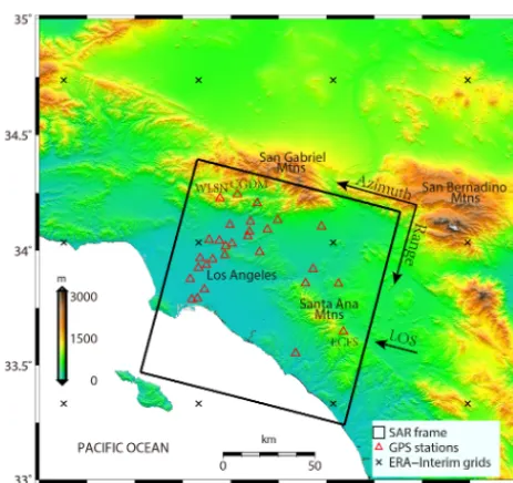
We carried out the study using data sets collected in the Los Angeles basin, located in southern California, USA. This study area neighbours the Pacific Ocean in the west and south-west, thus is rich with atmospheric water vapour and is well covered by a dense network of continuous GPS re-ceivers. These conditions make it particularly suitable for atmospheric water vapour studies. Figure 1 shows the to-pography map of the study area. A set ofN=8 ENVISAT ASAR SLC (Advanced Synthetic Aperture Radar Single Look Complex) images were acquired over this region for the period between 6 October 2007 to 29 November 2008. The image was acquired during descending passes, Track 170, with the average look angleθ=22.6◦. Actually, the value of look angleθ varies over the SAR scene from near range to far range between 16.5 and 23.2◦. Accuracy may improve if local look angle of every pixels within interferogram is con-sidered when calculating the mapping function. We used the average look angle in our study. The acquisition time was 18:01 UTC. For SAR interferometric processing, an external DEM with 30 m height postings from Shuttle Radar Topog-raphy Mission (SRTM) (Farr et al., 2007) was used for re-moving the influence of topography and the Earth’s curva-ture, while the precise orbit information from Delft Institute for Earth-Oriented Space Research was utilized for minimiz-ing the orbital errors. The black square in Fig. 1 shows the footprint of SAR images.
Figure 1. The topography map of the study area. The red trian-gles represent the locations of GPS stations. The locations of GPS stations CGDM, ECFS and WLSN are indicated. The black box defines the area of ENVISAT ASAR images. Black crosses indicate the position of the ERA-Interim model grid nodes used in this study. The arrow on the right side of the SAR frame indicates the line of sight (LOS) of the radar signal.
GPS data and produce position solutions for stations in the PBO network as well as other selected stations. One AC is operated by the Geodesy Laboratory at Central Washington University (CWU) and uses the GIPSY/OASIS-II process-ing package. The other AC is located at the New Mexico Institute of Technology (NMT) and uses GAMIT/GLOBK. The Analysis Centres provide tropospheric data products, in-cluding zenith atmospheric delay, that are archived at the UNAVCO Data Center and are openly and freely available (http://www.unavco.org/data/data.html). The availability of GPS measurements also allowed us to separate possible sur-face deformation from the atmospheric signals in differential interferograms. The red triangles in Fig. 1 represent the loca-tions of GPS staloca-tions.
The ERA-Interim reanalysis from the European Centre for Medium-Range Weather Forecasts (ECMWF) is used to produce maps of hydrostatic delay and water vapour con-version factor. ERA-Interim is a global atmospheric model which was conceived to address some of the problems seen in ERA-40 (Dee et al., 2011). It is based on 4-dimensional variational assimilation of global surface and satellite meteo-rological data. The outputs of ERA-Interim used in our study are estimates of temperature, specific humidity and geopo-tential height, defined at 37 pressure levels (1000–1 hPa), and a spatial resolution of 0.75◦ (∼75 km). The black crosses in Fig. 1 show the distribution of ERA-Interim model grid nodes used in this study. The MERIS is located together with
the ASAR sensor on board the ENVISAT satellite (Bennartz and Fischer, 2001), thus the simultaneous water vapour mea-surements from MERIS were used as a reference data for comparison and evaluation.
3 Estimating PWV from InSAR
Here, we present the methods for obtaining zenith wet de-lay from SAR interferogram and converting it to PWV. In Sect. 3.1, the retrieval of zenith wet delay from the SAR in-terferogram is described. Section 3.2 describes the method for computing the conversion factor required to map the zenith wet delay onto PWV by using ERA-Interim reanal-ysis. In Sect. 3.3, the approach for calibrating the PWV esti-mated from InSAR using GPS observations is discussed. 3.1 Atmospheric delay in InSAR
The unwrapped interferometric phase for each pixel in an in-terferogram is given by the superposition of several compo-nents including topography, Earth surface displacement and atmosphere. It can be written as follows:
∅int=∅topo+∅defo+∅orb+∅atm+∅noise, (1)
where ∅topo is the phase contribution from land
topogra-phy, ∅defo represents the ground deformation between the
acquisitions,∅orbcounts for the phase caused by inaccurate
satellite orbit,∅atmindicates the atmospheric state variations
during SAR acquisitions and∅noise denotes the noise
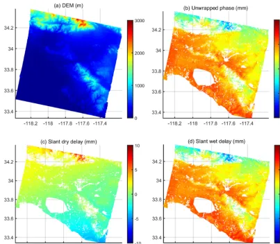
Figure 2. (a)Regional land topography from SRTM at interferogram pixels.(b)Unwrapped phase of differential interferogram (master image from 16 August 2008, slave image from 25 October 2008).(c)Slant hydrostatic delay difference maps predicted from the ERA-Interim model.(d)Slant wet delay difference obtained by subtracting(c)from(b). The rapidly subsiding areas are masked out in(b),(c) and(d).
(Doin et al., 2009)
∅trop=∅hyd+∅wet, (2)
where ∅hyd(z)= −
4π λcosθinc
10−6
k1Rd
g0
P (z)−P (z0)
(3)
∅wet(z)= −
4π λcosθinc
10−6 zref
Z
z
k2−
Rd
Rv
k1 e(z)
T (z)+k3 e(z) T (z)2
dz. (4)
The hydrostatic delay ∅hyd is calculated using the specific
gas constant for hydrostatic airRd, the local gravityg0at the
mass centre of the atmospheric column between zandzref
and air pressureP. The wet delay∅wetis computed using the
partial pressure of water vapoure, water vapour specific gas
constantRv and temperature T. zref represents a reference
height (30 km used in this study) above which the delay is assumed to be nearly unchanged with time. The atmospheric refractivity constantsk1,k2andk3are determined in Smith
and Weintraub (1953) andk2−RRd
vk1
is often namedk02= 0.233 K Pa−1.λis the radar wavelength and−4π
λ is a scale factor to convert the delay in millimetre into phase in radian.
θinc is the radar incidence angle and the factor cos(θ1
inc) is a
mapping function applied to project the delay from the zenith direction to the radar line of sight (LOS). The constants in Eqs. (3) and (4) are listed in Table 2.
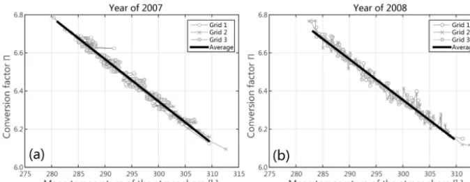
re-Figure 3.Conversion factor5estimated based on the water vapour partial pressure and temperature extracted at three ERA-Interim model grids located within the SAR scene (see Fig. 1). The black line is the linear regression between the averaged conversion factors and the mean temperature. The measurements were taken at 18:00 UTC (close to the SAR acquisition time of 18:01 UTC, making the time difference between these two data sets negligible) over 120 days (10 days/month) in the years 2007(a)and 2008(b).
sults in a spatially variable signal in the hydrostatic delay (Mateus et al., 2013b). The variation of hydrostatic delay depending on the topography could be up to 15 mm in our study area. Therefore, in order to accurately derive the wet delay, the hydrostatic delay must be precisely estimated and subtracted from the total tropospheric delay. This delay can be calculated if the atmospheric pressure is known along the signal propagation path or along the zenith direction. In this work, we used the vertical profiles of atmospheric pressure provided by ERA-Interim reanalysis products to predict this component of hydrostatic delay. We interpolated the atmo-spheric pressure onto altitude profiles on each ERA-Interim model grid using a spline interpolation and calculated the hydrostatic delay using Eq. (3). The resulting vertical pro-files of hydrostatic delay were horizontally interpolated to the resolution of SAR interferogram using a bilinear interpo-lation. We also used the outputs of temperature and relative humidity from the ERA-Interim model to produce the maps of water vapour conversion factor using the same interpola-tion strategy; this will be discussed in next subsecinterpola-tion. The map of hydrostatic delay is displayed in Fig. 2c. This delay represents a long-wavelength signal, is smooth in space and rose up to 1 cm on the mountain areas. The slant wet delay (Fig. 2d) was obtained by subtracting the hydrostatic delay from the total tropospheric delay. The slant wet delay differ-ence in LOS was converted to the zenith wet delay differdiffer-ence (1ZWD)in millimetres using a simple mapping function:
1ZWDInSAR= −
λcosθinc
4π ∅wet. (5)
3.2 Conversion of ZWD into PWV
The zenith wet delay is considered to be a measurement of the water vapour content in the atmosphere. The relationship between the ZWD and PWV can be expressed as follows (Bevis et al., 1994):
PWV=κ×ZWD or ZWD=5×PWV, (6)
whereκ is the water vapour conversion factor and5=κ−1
is calculated by the following equation:
5=10−6ρRv
k3
Tm +k2−
Rd
Rv
k1, (7)
whereρis the density of the liquid water (listed in Table 2).
Tmis the weighted mean temperature of the atmosphere and
is related to the surface temperatureTsin degrees Kelvin
(Be-vis et al., 1992).
Tm≈70.2+0.72×Ts (8)
Using this relationship to estimateTmwill produce
approxi-mately 2 % error in PWV (Bevis et al., 1992). The most ac-curate way to compute the mean temperature is to calculate the following integral equation between the ground surface
z0and the reference heightzref, given by (Davis et al., 1985)
Tm= Rzref
z0
e T
dz
Rzref
z0
e T2
dz
. (9)
The value of5is dimensionless and usually ranges from 6.0 to 6.5 (and could be up to 7.0 in some circumstances) (Bevis et al., 1992). For the purpose of rough conversion between ZWD and PWV, an empirical constant5=6.25 (κ=0.16)
was used. However, the actual value ofκ changes with wa-ter vapour pressure and temperature, then minor errors inκ
profiles of temperature and relative humidity. The relative hu-midity is converted to partial pressure of water vapoureby a mixed Clausius–Clapeyron equation (Jolivet et al., 2011). To evaluate the sensitivity of5to the weighted mean tem-peratureTm, its values are computed over 120 days (10 days
in one month) in the years 2007 and 2008. Figure 3 plots
5 against the averageTmfor the three ERA-Interim model
grids (indicated as the black crosses in Fig. 1) located within the SAR scene. From Fig. 3, we observed that the value of5
changes withTm, and5is in the range of 6.09 to 6.79 in the
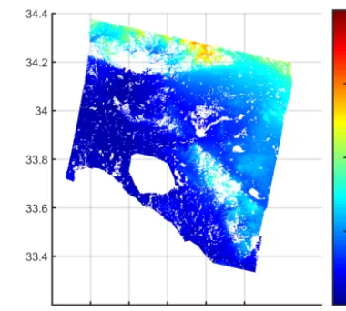
year of 2007 (Fig. 3a), whereas it varies between 6.17 and 6.74 in the year of 2008 (Fig. 3b). The fitted average curves linearly decrease with rates of−0.0214 and−0.0221/K re-spectively. As expected the value of 5 is much higher on winter days (low temperature) than summer days (high tem-perature). On the other hand, since the temperature gener-ally decreases with altitude in the troposphere, the conver-sion factor is correlated with the elevation. Therefore, us-ing the empirical value ofκ=0.16 is not appropriate for the whole study area; rather its value is calculated using global atmospheric model ERA-Interim. Figure 4 shows the spatial distribution map of5on 16 August 2008 produced by ERA-Interim. It can be seen that the value of 5 varies spatially and it has a higher value on the mountainous areas than those areas with a flat terrain. We then averaged the spatial maps of 5 at the two interferometric acquisition times to derive the conversion factors for mapping the wet delay onto water vapour.
3.3 InSAR PWV calibrated by GPS PWV
PWV estimated from GPS is not directly comparable with
1PWV estimated from InSAR. The unwrapping procedure introduces an arbitrary constant in the unwrapped phase, so the InSAR technique can just measure the 1PWV with an unknown bias, whereas the GPS-based1PWV is unbiased. To resolve this problem,1PWV maps derived from InSAR are calibrated by GPS-based1PWV. It should be noted that only the signals from satellites with elevation angle larger than the cut-off elevation angle are recorded by the GPS re-ceiver. Thus, the PWV estimates from GPS are derived by being weighted with the elevation and azimuth angles of the individual ray paths from the GPS satellites to the receiver. Figure 5 shows the schematic diagram of this effect. The cut-off elevation angle is set to 15◦and assumes the water vapour is concentrated in the lower part (1.4 km) of the troposphere; the corresponding cone radius is approximately 5.4 km. All observations outside this cone are discarded. We averaged the
1PWV values of the interferogram pixels located within the corresponding circular area before comparing InSAR mea-surements to that of GPS. We calculated the temporal dif-ference of the PWV at each GPS station, at about the same acquisition time as the two interferometric SAR images. The InSAR1PWV calibration process is to determine the con-stantK by minimizing the following cost function (Mateus
Figure 4.The spatial distribution of conversion factor5calculated based on ERA-Interim. It is calculated at the time 18:00 UTC on 16 August 2008.
et al., 2013a). NGPS X k=1
1PWVGPSk − 1
Np(k)
Np(k)
X
i=1
1PWVInSARi +K
2
, (10)
whereNGPS is the number of GPS receivers, Np(k)is the
number of InSAR pixels located within the circular area around thekth GPS receiver,1PWVGPSk is the temporal dif-ference of PWV between master and slave dates by GPS,
1PWVInSARi represents the 1PWV estimated by InSAR. Finally, the relative map of the1PWV from the interfero-grams were calibrated by subtracting the constantK from the1PWVInSARmap.
4 Results and discussion
Figure 5.GPS receiver records a satellite signal at a cut-off elevation angleθcutdefining a cone-like tropospheric section above the antenna. Forθcut=15◦,rc≈5.4 km. The1PWV estimated by InSAR pixels within this circle are averaged to emulate GPS-based1PWV.
Figure 6.Time series over 24 h of PWV estimated from GPS observations at 29 GPS stations located in the study area (as shown in Fig. 1) on four SAR acquisition dates. The vertical black dashed lines represent the SAR satellite overpass time (18:01 UTC). Black arrows on each plot indicate the locations of GPS station WLSN (altitude about 1700) on Mount Wilson. In general, the higher the GPS station, the lower the PWV value.
vapour measurements and also inspect their spatial distribu-tion properties.
4.1 GPS PWV measurements
The tropospheric products analysed by CWU at the 29 GPS stations (Fig. 1) are used in this study. These products pro-vide the zenith tropospheric delay at each GPS station every 5 min. The high temporal sampling of GPS measurements enables us to obtain the zenith wet delay at a time as close as possible to the SAR image acquisition time. The cut-off ele-vation angle (θcut=15◦) was considered in the GPS data
pro-cessing. The Saastamoinen model and gridded Vienna Map-ping Function (VMF1GRID) (Kouba, 2007) were used for calculating a priori values of zenith hydrostatic delay. The
zenith wet delay was then obtained by subtracting the zenith hydrostatic delay from the total delay and the PWV was fi-nally obtained by Eq. (6) using the water vapour conversion factor estimated from ERA-Interim reanalysis products.
Table 1.Acquisition dates of master and slave images and their parameter information.
Number Master Slave Normal baseline Temporal baseline Height ambiguity
(DDMMYYYY) (DDMMYYYY) (m) (days) (m)
1 6 October 2007 15 December 2007 −62.75 70 146.83
2 6 October 2007 19 January 2008 36.16 105 254.84
3 15 December 2007 19 January 2008 98.34 35 93.77
4 19 January 2008 3 May 2008 −51.85 105 177.05
5 3 May 2008 7 June 2008 217.11 35 42.54
6 3 May 2008 16 August 2008 −191.01 105 48.30
7 7 June 2008 16 August 2008 −27.67 70 333.19
8 16 August 2008 25 October 2008 31.72 70 290.90
9 16 August 2008 29 November 2008 −4298.42 105 30.92
10 25 October 2008 29 November 2008 −284.21 35 32.48
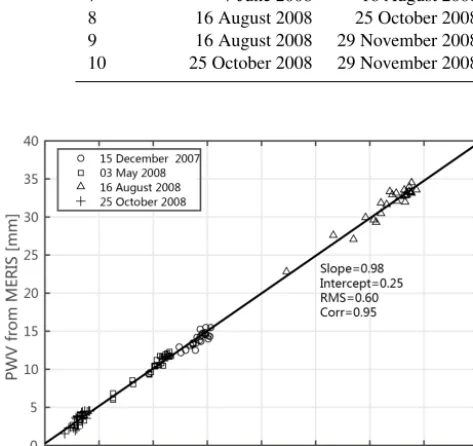
Figure 7.MERIS PWV against GPS PWV at 29 stations on 4 days of ENVISAT overpass time. The MERIS observations are averaged within circles of 5.4 km radius centred on the GPS station.
Table 2.Constants used for calculating atmospheric delay (Smith and Weintraub, 1953).
Constant Value
Rd 287.05 J kg−1K−1 Rv 461.95 J kg−1K−1
g0 9.81 ms−2
k1 0.776 K Pa−1
k2 0.716 K Pa−1
k3 3.75×10³K2Pa−1
ρ 1000 kg m−3
In Fig. 7, we plot PWV measurements derived from MERIS against PWV results estimated from GPS at 29 sta-tions on the 4 SAR acquisition days (in Fig. 6). Since GPS PWV estimates represent average values over the reversed cone with a ∼5.4 km radius base, we averaged the PWV from MERIS within the circular area around the locations of
the GPS stations. The result shows a strong correlation (0.95) between GPS and MERIS. The mean absolute error (MAE) of the differences between the two data sets does not exceed 0.5 mm and the root mean square (rms) value is 0.60 mm. The slope of the line in Fig. 7 is 0.98. Similar comparison was performed and the MERIS was validated to be the most accurate tool to map PWV at high resolution and was in prin-ciple particularly useful for InSAR tropospheric delay miti-gation (Cimini et al., 2012). Thus GPS and MERIS measure-ments of water vapour are in good agreement and we should not expect a perfect correlation between the two data sets be-cause we averaged the conical effect of GPS with a circle and there is noise in both data sets.
4.2 InSAR1PWV measurements
spa-Table 3.Assessment of1PWV maps obtained by InSAR after calibration of offset using GPS (master image from 16 August 2008, slave image from 25 October 2008). For each GPS station, PWV differences from GPS between master and slave SAR acquisition times are computed and compared to the average values of InSAR estimates at pixels located within a circular area of 5.4 km around each GPS station. Differences are summarized in the last column. MAE and SD represent the mean absolute error and standard deviation.
Number GPS Longitude Latitude 1PWVGPS 1PWVInSAR Difference
station (◦) (◦) (mm) (mm)
Mean (mm) SD (mm)
1 AZU1 −117.896 34.126 28.94 28.62 0.65 0.32
2 BGIS −118.159 33.967 30.15 29.92 0.47 0.23
3 BKMS −118.094 33.962 29.89 29.64 0.28 0.25
4 CCCO −118.211 33.876 29.50 30.26 0.43 −0.76
5 CGDM −117.964 34.243 25.13 27.02 1.47 −1.89
6 CNPP −117.608 33.857 30.87 29.84 1.37 1.03
7 CVHS −117.901 34.082 29.10 28.66 0.42 0.44
8 DYHS −118.125 33.937 29.03 29.50 0.30 −0.47
9 ECFS −117.411 33.647 24.51 26.03 1.22 −1.52
10 EWPP −117.525 34.104 26.71 25.98 0.46 0.73
11 GVRS −118.112 34.047 28.83 29.84 0.34 −1.01
12 HOLP −118.168 33.924 29.53 29.77 0.50 −0.24
13 LBC1 −118.137 33.832 30.29 29.78 0.32 0.51
14 LBC2 −118.173 33.791 29.31 29.68 0.32 −0.37
15 LBCH −118.203 33.787 29.22 29.62 0.37 −0.40
16 LONG −118.003 34.111 31.31 31.23 0.35 0.08
17 LORS −117.754 34.133 26.58 26.82 0.79 −0.24
18 MAT2 −117.436 33.856 28.24 28.35 0.87 −0.11
19 NOCO −117.569 33.919 30.77 29.51 0.90 1.26
20 PSDM −117.807 34.091 28.30 27.79 0.45 0.51
21 RHCL −118.026 34.019 28.53 29.36 0.64 −0.83
22 SBCC −117.661 33.553 30.72 30.51 0.54 0.21
23 SGDM −117.861 34.205 27.87 27.15 1.16 0.72
24 SPMS −117.848 33.992 28.14 28.56 0.51 −0.42
25 VYAS −117.992 34.030 30.39 29.24 0.52 1.15
26 WCHS −117.911 34.061 30.38 29.74 0.44 0.64
27 WHC1 −118.031 33.979 29.66 29.21 0.64 0.45
28 WLSN −118.055 34.226 18.08 20.92 1.61 −2.84
29 WNRA −118.059 34.043 30.34 29.68 0.45 0.66
MAE 0.70
SD 0.96
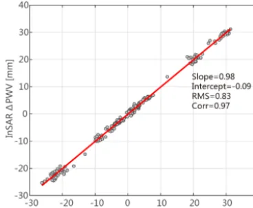
Figure 10.Scatter plot of1PWV from GPS and InSAR. The data points (grey circles) are from Fig. 9.
tial resolution of the interferograms to 160 m×160 m. The wrapped phases were unwrapped using a branch cut algo-rithm (Goldstein et al., 1988) and possible orbital errors were corrected by network de-ramping method. Oscillator drifts induce a systematic phase ramp in the interferogram from the ENVISAT satellite (Marinkovic and Larsen, 2015), they were removed by the script provided in the StaMPS software. The local rapid ground subsiding region was masked out. The wet delay differences of InSAR were obtained by subtract-ing the component of hydrostatic delay predicted from the ERA-Interim model. The wet delay differences were finally mapped onto1PWV maps using the water vapour conver-sion factor as explained in Sect. 3.2.
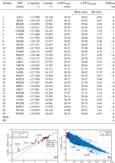
Due to the fact that the unwrapped processing introduced an arbitrary constant into the phase, all the 1PWV maps from InSAR were relative measurements. Therefore, we need the calibration by using the ground measurements of PWV from GPS. The GPS PWV values were estimated from the zenith wet delay provided by the CWU data analysis cen-tre as described in previous section. The overpass time of ENVISAT satellite was 18:01 UTC, thus we computed the temporal difference of the PWV at each GPS station at time 18:00 UTC, making the time differences negligible. Using the1PWV estimates from GPS, the1PWV maps of InSAR were calibrated by solving the cost function (Eq. 10) as de-scribed in Sect. 3.3. A comparison of the calibrated1PWV from the interferogram (master image from 16 August 2008, slave image from 25 October 2008, see Fig. 2) and1PWV from the 29 GPS stations is displayed in Fig. 8a. The slope of the line in this figure is 0.73 while the correlation coefficient is 0.95, suggesting the GPS and InSAR measurements of PWV are in reasonable agreement, although there is noise in both data sets. Figure 8b plots the1PWV from GPS and In-SAR as a function of elevation. This plot shows that the con-tent of water vapour is significantly dependent on the terrain height. The dependence on height of1PWV is roughly lin-ear or better exponential as the concentration of water vapour
generally decreases linearly or exponentially with elevation (Basili et al., 2014). However, since we obtained the water vapour difference between two SAR acquisitions, it may hap-pen that1PWV can decrease but also increase with height. The decreasing trend in Fig. 8b implies that the absolute wa-ter vapour content was smaller at the acquisition time of the slave image than at the acquisition time of the master image. The quantitative comparison of this interferogram is sum-marized in Table 3. It can be seen that most of differences are smaller than 2 mm. The MAE of1PWV between GPS and InSAR is 0.70 mm and the rms value is 0.91 mm. It is worth noting that large differences between InSAR and GPS at stations CGDM, ECFS and WLSN (indicated by the black arrows in Fig. 8) were observed, and the largest difference (−2.84 mm) was observed at station WLSN. The standard deviations of InSAR pixels located within the circular area around these three GPS stations also show a high value (the fourth column in Table 3). The three GPS stations are lo-cated in mountain areas with an altitude 730, 820, 1700 m for the CGDM, ECFS and WLSN stations respectively. This interferogram also shows a high value for height ambiguity (290.90 m). Therefore, we can conclude that the large dis-crepancies between InSAR and GPS for these three stations are most probably due to the topographic phase error during interferometric processing.
The comparisons of1PWV from the two techniques at each GPS station for the 10 interferograms are shown in Fig. 9. A good agreement between the InSAR and GPS was found across the whole data set. Large differences between InSAR and GPS at stations CGDM, ECFS and WLSN were also found on those interferograms with a high value of height ambiguity (interferograms 1, 2, 4 and 7 in Table 1). In Fig. 10, we put all the data points in a scatter plot. The rms difference of InSAR1PWV with respect to the GPS
1PWV is better than 1 mm, and the correlation is 0.97. The PWV estimates from the two techniques are characterized by different sampling properties both in space and time. GPS can provide an absolute value of the PWV every 5 min but refers to the parts of atmosphere observed within a cone with a radius depending on the elevation cut-off angle, whereas InSAR gives a high-spatial-resolution map of the1PWV with a time separation of 35 days or more. The high tempo-ral sampling of GPS and high spatial resolution of InSAR are complementary for numerical weather modelling, which will improve the model resolution and give a better understanding of the structure of atmospheric patterns.
4.3 Validation using water vapour measurements from MERIS
pix-Figure 11.
els by MERIS acquired simultaneously with the ENVISAT ASAR images. The water vapour content is expressed as inte-grated water vapour (IWV) in the MERIS products. The the-oretical accuracy of the MERIS IWV under cloud-free condi-tions over land is 0.16 g m−2(Bennartz and Fischer, 2001) at full resolution (∼300 m), which corresponds to 1.6 mm ac-curacy in PWV. This acac-curacy will deteriorate under cloudy conditions or over water surfaces. The percentage of cloud-free conditions for MERIS data we used in this study are larger than 90 % except for the image acquired on 29 Novem-ber 2008 having a coverage percentage of 80 %. For the sake of comparison, we built differences of PWV maps (1PWV)
from MERIS. This is performed based on the software
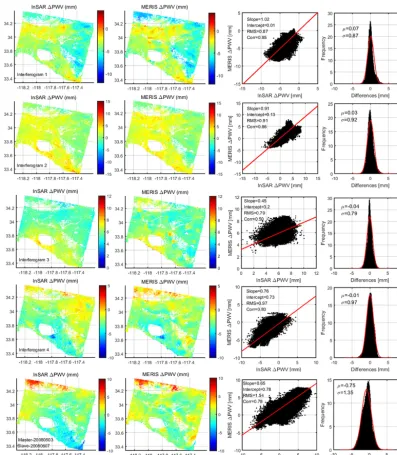
pack-age called TRAIN (Toolbox for Reducing Atmospheric In-SAR Noise) (Bekaert et al., 2015). Figure 11 shows the cali-brated1PWV maps derived from the 10 interferograms (in Table 1) and the corresponding1PWV maps from MERIS data. The first column shows the1PWV derived from In-SAR that has been calibrated with GPS observations. The
Figure 11.Comparison of the1PWV maps derived from InSAR and MERIS. For all images here, the root mean square (rms), correlation (Corr), differential mean (µ)and standard deviation (σ )are computed.
square (rms), mean (µ), and standard deviation (σ ) of the differences between the two data sets. From visual compari-son, InSAR1PWV and MERIS1PWV show a large spa-tial correspondence. Furthermore, the quantitative compar-isons indicate high-correlation coefficients (Corr > 0.7) be-tween the two data sets, except for interferogram 3 (master image from 15 December 2007, slave image from 19 January 2008) and interferogram 9 (master image from 16 August 2008, slave image from 29 November 2008) having correla-tion coefficients of Corr=0.5 and Corr=0.67 respectively. The differences between the InSAR and MERIS maps
fol-low a Gaussian distribution with mean values close to zero and standard deviations less than 2 mm.
5 Conclusion
ERA-Interim reanalysis products. We also used the outputs from the ERA-Interim model to produce maps of the conversion factor for mapping zenith wet delay onto PWV at each pixel in the radar scene. All maps of1PWV derived from inter-ferograms were calibrated using a network of 29 continuous GPS stations located in the SAR scene. The PWV estimates from InSAR and MERIS show strong agreement with the data from GPS. Since the GPS PWV estimates represent the average of the tropospheric effect within a cone above the re-ceiver, InSAR and MERIS pixels were aggregated to enable a proper comparison. The comparative analysis between In-SAR and MERIS1PWV maps demonstrates strong spatial correlation with a less than 2 mm standard deviation of differ-ence. Our study demonstrates that satellite synthetic aperture radar interferometry can be applied to study the spatial distri-bution of the PWV with a spatial resolution of 160 m and an accuracy of∼2 mm. This advantage of InSAR provides un-surpassed insights for capturing the small-scale water vapour distribution. This property could be important for numerical weather forecasting models. Furthermore, forecasting mod-els could take advantage of this source of water vapour maps to enhance the accuracy of their assimilation systems. In turn, the more accurate atmospheric prediction models are benefi-cial for correcting the tropospheric delay affected by water vapour in the applications of geodesy.
6 Data availability
The ENIVISAT ASAR datasets were provided by ESA through Dragon-3 project (id10569). The GPS tropospheric products are archived at the UNAVCO Data Center (2016) and are openly and freely available at http://www.unavco. org/data/data.html. The 30 m SRTM DEM were downloaded from USGS EarthExplorer (2016) (http://earthexplorer.usgs. gov/). The ERA-Interim reanalysis came from the web-site of ECMWF (2016) (http://www.ecmwf.int/en/research/ climate-reanalysis/era-interim).
Acknowledgements. The authors thank ESA for the ENVISAT ASAR images and MERIS data. The authors would like to thank the GPS data provider: UNAVCO Data Center. This work was jointly supported by the National Natural Science Foundation of China (grant no. 61331016), the National Key Basic Research Program of China (grant no. 2013CB733205) and the Shanghai Academy of Spaceflight Technology Innovation Fund (grant no. SAST201321). I would also like to thank Stephen C. McClure for his helpful comments and suggestions on this manuscript.
Edited by: S. Mori
Reviewed by: two anonymous referees
References
Basili, P., Bonafoni, S., Ciotti, P., and Pierdicca, N.: Modeling and Sensing the Vertical Structure of the Atmospheric Path Delay by Microwave Radiometry to Correct SAR Interferograms, IEEE T. Geosci. Remote, 52, 1324–1335, 2014.
Beauducel, F., Briole, P., and Froger, J.-L.: Volcano-wide fringes in ERS synthetic aperture radar interferograms of Etna (1992– 1998): Deformation or tropospheric effect?, J. Geophys. Res., 105, 16391–16402, 2000.
Bekaert, D. P. S., Walters, R. J., Wright, T. J., Hooper, A. J., and Parker, D. J.: Statistical comparison of InSAR tropospheric cor-rection techniques, Remote Sens. Environ., 170, 40–47, 2015. Bennartz, R. and Fischer, J.: Retrieval of columnar water vapour
over land from backscattered solar radiation using the Medium Resolution Imaging Spectrometer, Remote Sens. Environ., 78, 274–283, 2001.
Bevis, M., Businger, S., Herring, T. A., Rocken, C., Anthes, R. A., and Ware, R. H.: GPS meteorology : Remote sensing of atmo-spheric water vapor using the global positioning system, J. Geo-phys. Res., 97, 15787–15801, 1992.
Bevis, M., Businger, S., Chiswell, S., Herring, T. A., Anthes, R. A., Rocken, C., and Ware, R. H.: GPS meteorology: Mapping zenith wet delays onto precipitable water, J. Appl. Meteorol., 33, 379– 386, 1994.
Cimini, D., Pierdicca, N., Pichelli, E., Ferretti, R., Mattioli, V., Bonafoni, S., Montopoli, M., and Perissin, D.: On the accuracy of integrated water vapor observations and the potential for miti-gating electromagnetic path delay error in InSAR, Atmos. Meas. Tech., 5, 1015–1030, doi:10.5194/amt-5-1015-2012, 2012. Davis, J. L., Herring, T. A., Shapiro, I. I., Rogers, A. E. E., and
Elgered, G.: Geodesy by radio interferometry: Effects of atmo-spheric modeling errors on estimates of baseline length, Radio Sci., 20, 1593–1607, 1985.
Dee, D. P., Uppala, S. M., Simmons, A. J., Berrisford, P., Poli, P., Kobayashi, S., Andrae, U., Balmaseda, M. A., Balsamo, G., Bauer, P., Bechtold, P., Beljaars, A. C. M., van de Berg, L., Bid-lot, J., Bormann, N., Delsol, C., Dragani, R., Fuentes, M., Geer, A. J., Haimberger, L., Healy, S. B., Hersbach, H., Hólm, E. V., Isaksen, L., Kållberg, P., Köhler, M., Matricardi, M., McNally, A. P., Monge-Sanz, B. M., Morcrette, J. J., Park, B. K., Peubey, C., de Rosnay, P., Tavolato, C., Thépaut, J. N., and Vitart, F.: The ERA-Interim reanalysis: configuration and performance of the data assimilation system, Q. J. Roy. Meteor. Soc., 137, 553–597, 2011.
Doin, M. P., Lasserre, C., Peltzer, G., Cavalié, O., and Doubre, C.: Corrections of stratified tropospheric delays in SAR interferom-etry: Validation with global atmospheric models, J. Appl. Geo-phys., 69, 35–50, 2009.
ECMWF: ERA-Interim reanalysis, available at: http://www.ecmwf. int/en/research/climate-reanalysis/era-interim, last access: 8 September 2016.
Farr, T. G., Rosen, P. A., Caro, E., Crippen, R., Duren, R., Hens-ley, S., Kobrick, M., Paller, M., Rodriguez, E., Roth, L., Seal, D., Shaffer, S., Shimada, J., Umland, J., Werner, M., Oskin, M., Bur-bank, D., and Alsdorf, D.: The Shuttle Radar Topography Mis-sion, Rev. Geophys., 45, doi:10.1029/2005RG000183, 2007. Goldstein, R. M. and Werner, C. L.: Radar interferogram
Goldstein, R. M., Zebker, H. A., and Werner, C. L.: Satellite radar interferometry: Two-dimensional phase unwrapping, Radio Sci., 23, 713–720, 1988.
Hanssen, R.: “Radar interferometry”, in: Data Interpretation and Er-ror Analysis, Delft Univ. Technol., Delft, the Netherlands, 2001. Hooper, A., Segall, P., and Zebker, H.: Persistent scatterer interfer-ometric synthetic aperture radar for crustal deformation analysis, with application to Volcán Alcedo, Galápagos, J. Geophys. Res., 112, doi:10.1029/2006JB004763, 2007.
Jolivet, R., Grandin, R., Lasserre, C., Doin, M. P., and Peltzer, G.: Systematic InSAR tropospheric phase delay corrections from global meteorological reanalysis data, Geophys. Res. Lett., 38, doi:10.1029/2011GL048757, 2011.
Jolivet, R., Agram, P. S., Lin, N. Y., Simons, M., Doin, M.-P., Peltzer, G., and Li, Z.: Improving InSAR geodesy using Global Atmospheric Models, J. Geophys. Res.-Sol. Ea., 119, 2324– 2341, 2014.
Kampes, B. M., Hanssen, R. F., and Perski, Z.: Radar interferometry with public domain tools, Frascati, Italy, 1–5, 2003.
Kouba, J.: Implementation and testing of the gridded Vienna Map-ping Function 1 (VMF1), J. Geodesy, 82, 193–205, 2007. Li, Z. H., Muller, J. P., and Cross, P.: Comparison of
precip-itable water vapor derived from radiosonde, GPS, and Moderate-Resolution Imaging Spectroradiometer measurements, J. Geo-phys. Res., 108, doi:10.1029/2003JD003372, 2003.
Liao, M., Jiang, H., Wang, Y., Wang, T., and Zhang, L.: Improved topographic mapping through high-resolution SAR interferome-try with atmospheric effect removal, ISPRS J. Photogramm., 80, 72–79, 2013.
Marinkovic, P. and Larsen, Y.: On resolving the local oscillator drift induced phase ramps in ASAR and ERS1/2 interferometric data – the final solution, Fringe 2015 workshop, 23–27 March 2015, Frascati, Italy, 318, 2015.
Mateus, P., Nico, G., and Catalão, J.: Can spaceborne SAR interfer-ometry be used to study the temporal evolution of PWV?, Atmos. Res., 119, 70–80, 2013a.
Mateus, P., Nico, G., Tome, R., Catalao, J., and Miranda, P. M. A.: Experimental study on the atmospheric delay based on GPS, SAR interferometry, and numerical weather model data, IEEE T. Geosci. Remote, 51, 6–11, 2013b.
UNAVCO Data Center: GPS tropospheric products, available at: http://www.unavco.org/data/data.html, last access: 8 September 2016.
USGS EarthExplorer: SRTM DEM, available at: http: //earthexplorer.usgs.gov/, last access: 8 September 2016. Smith, E. K. and Weintraub, S.: The constants in the equation for
atmospheric refractive index at radio frequencies, Proceedings of the IRE, 41, 1035–1037, 1953.