A. Gnanadesikan1, M.-A. Pradal1, and R. Abernathey2
1Department of Earth and Planetary Sciences, Johns Hopkins University, Baltimore, MD, USA 2Department of Earth and Environmental Sciences, Columbia University, New York, NY, USA Correspondence to: A. Gnanadesikan ([email protected])
Received: 11 October 2014 – Published in Ocean Sci. Discuss.: 20 November 2014 Revised: 10 June 2015 – Accepted: 27 June 2015 – Published: 27 July 2015
Abstract. This paper uses a suite of Earth system models which simulate the distribution of He isotopes and radio-carbon to examine two paradoxes in Earth science, each of which results from an inconsistency between theoretically motivated global energy balances and direct observations. The helium–heat paradox refers to the fact that helium emis-sions to the deep ocean are far lower than would be expected given the rate of geothermal heating, since both are thought to be the result of radioactive decay in Earth’s interior. The isopycnal mixing paradox comes from the fact that many the-oretical parameterizations of the isopycnal mixing coefficient ARedithat link it to baroclinic instability project it to be small
(of order a few hundred m2s−1) in the ocean interior away
from boundary currents. However, direct observations using tracers and floats (largely in the upper ocean) suggest that values of this coefficient are an order of magnitude higher. Helium isotopes equilibrate rapidly with the atmosphere and thus exhibit large gradients along isopycnals while radiocar-bon equilibrates slowly and thus exhibits smaller gradients along isopycnals. Thus it might be thought that resolving the isopycnal mixing paradox in favor of the higher obser-vational estimates ofARedimight also solve the helium
para-dox, by increasing the transport of mantle helium to the sur-face more than it would radiocarbon. In this paper we show that this is not the case. In a suite of models with different spatially constant and spatially varying values ofARedi the
distribution of radiocarbon and helium isotopes is sensitive to the value of ARedi. However, away from strong helium
sources in the southeastern Pacific, the relationship between the two is not sensitive, indicating that large-scale advection is the limiting process for removing helium and radiocarbon from the deep ocean. The helium isotopes, in turn, suggest
a higher value ofARedi below the thermocline than is seen
in theoretical parameterizations based on baroclinic growth rates. We argue that a key part of resolving the isopycnal mixing paradox is to abandon the idea thatARedihas a direct
relationship to local baroclinic instability and to the so-called “thickness” mixing coefficientAGM.
1 Introduction
Because the ocean is highly stratified and weakly forced, tracer mixing occurs predominantly along surfaces of con-stant neutral density (Ledwell et al., 1998). The turbulent flux associated with mesoscale eddies is usually parameterized as downgradient eddy diffusion with a coefficientARedi(Redi,
1982; Griffies et al., 1998). Considering only one dimension for simplicity, the meridional flux of some tracerCalong an isopycnal is then
FC=v0C0= −A
Redi
∂C
∂s, (1)
where the overline denotes an average (ensemble or time), vis the meridional velocity along the isopycnal and∂/∂sis a gradient oriented along that isopycnal. The size ofARedi
obviously has the potential to play a major role in determin-ing the rate of exchange between the interior of the ocean and the surface. It is generally assumed that all passive trac-ers experience the same value ofARedi, though it is not clear
that this should be the case for very short-lived tracers or in the presence of spatially variable sources and sinks.
This is in part because ARedi represents only one
dynami-cally important process associated with eddies. In addition to stirring fluid parcels along isopycnal surfaces, eddies act to flatten those isopycnal surfaces as a result of baroclinic instability, releasing available potential energy. This process was parameterized by Gent and McWilliams (1990) in terms of an “eddy Stokes drift” arising from correlations between the thickness of an isopycnal layerhand the velocitiesv. By analogy with Eq. (1) (again considering only the meridional dimension for simplicity),
v∗=v0h0/h= −AGM
∂h/∂y h
= −AGM
∂Sρy
∂z , (2)
wherev∗is the meridional velocity associated with the
over-turning eddies,AGM is the so-called “thickness diffusivity”
(in reality the diffusivity is implemented as a diffusivity in interface height) andSρyis the slope of isopycnal surfaces in theydirection. As described below, many published models use the following assumptions to constrainARedi.
1. It is equal toAGMbecause the same eddies accomplish
the mixing (Griffies, 1998).
2. It is therefore largest in boundary currents where eddy kinetic energy is most intense and baroclinicity is largest.
3. Because the size of the observed overturning circulation puts limits on how largeAGMcan be in these boundary
currents (Gnanadesikan, 1999),ARediis only on the
or-der of a few hundred square meters per second in the gyre interiors and in the deep ocean.
Examples of models which implement these assumptions in-clude GFDL CM2.0 (Geophysical Fluid Dynamics Labora-tory; Gnanadesikan et al., 2006), CSIRO Mk3.6, (Common-wealth Scientific and Industrial Research Organisation; Gor-don et al., 2010) NCAR CESM (National Center for Atmo-spheric Research–Community Earth System Model; Danaba-soglu et al., 2012) and NorESM (Norwegian Earth System Model Bentsen et al., 2013). In the GFDL ESM2G model (Dunne et al., 2012)AGMandARediare both given by a
baro-clinic growth rate parameterization but have different mini-mum values. Other models use relatively small constant val-ues forARedi, including the Hadley Centre’s HadCM3 and
HadGEM (500 m2s−1, Jones et al., 2011), GFDL CM2.1
(600 m2s−1, Gnanadesikan et al., 2006) and GFDL ESM2M
(also 600 m2s−1, Dunne et al., 2012).
However, these assumptions lead to a paradox. Observa-tional estimates ofARedibased on tracers and floats (largely
near the ocean surface) show very large values for this pa-rameter, in the range of thousands of square meters per sec-ond. Only a few models (the CMCC ESM of Fogli et al., 2009, and CNRM CM3 of Salas-Melia et al., 2005) use rel-atively large values of ARedi (2000 m2s−1in both cases) in
the ocean interior. We term this order of magnitude differ-ence between the values ifARediemerging from theory and
direct observations the isopycnal mixing paradox.
One reason this paradox has remained unresolved is that physical properties in ocean-only models are far less sen-sitive to ARedi than they are to AGM, as surfaces of
con-stant temperature, salinity and density often align with each other. However,ARedi can have a more significant impact
on the distribution of tracers that have interior sources and sinks. Measurements of such tracers thus offer the possibil-ity of constrainingARedi. Gnanadesikan et al. (2013)
demon-strated that ARedi had a first-order impact on the
distribu-tion of hypoxic waters within a suite of Earth system models and Gnanadesikan et al. (2015) show that it impacts anthro-pogenic carbon uptake.
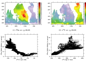
In this paper we expand on Gnanadesikan et al. (2013) to look at two other tracers.The first is primordial mantle helium-3. Incorporated into Earth’s interior when it formed, mantle helium is transported from the interior to regions where new ocean crust forms. This produces a strong helium isotope anomaly,
δ3He=(3He/4He)sample/(3He/4He)atm−1, (3)
as seen in Fig. 1a. As waters are brought to the surface, the helium exchanges rapidly with the atmosphere and the iso-topic signature is destroyed. The Pacific is enriched in man-tle helium both because waters are out of contact with the atmosphere in this basin for long periods of time (Khati-awala et al., 2012) and because the ridge centers in the Pacific spread faster, producing more new crust and degassing more
3He (Farley et al., 1995).
The second tracer is radiocarbon. Produced by galactic cosmic rays interacting with nitrogen in the upper atmo-sphere, radiocarbon equilibrates with the upper ocean on a relatively long timescale (of order 10 years for a 100 m deep layer). This equilibration is slow because air–sea gas exchange is controlled by the difference in pCO2, which
Figure 1. δ3He and radiocarbon in the ocean. (a)δ3He from Bianchi et al. (2010) onσ2 ( potential density relative to 2000 m minus 1000 kg m−3) of 36.95. (b)114C onσ2=36.95 from Key et al. (2004). (c) Vertically averagedδ3He vs. vertically averaged114C (2000– 5500 m). (d) Vertically averagedδ3He vs. radiocarbon age, 2000–5500 m, Pacific sector only.
stay at the surface long enough to have their radiocarbon re-set and so both deep and surface radiocarbon in the Southern Ocean lie in the range of−120 to−130 ‰. As waters flow into the Indian and Pacific oceans, radiocarbon continues to drop, with the lowest values (around−240 ‰) found in the North Pacific. While the above-air nuclear bomb tests added a significant amount of radiocarbon to the ocean–atmosphere system, relatively little of this is seen in the deep ocean (Key et al., 2004).
The relationship between deep radiocarbon (averaged be-low 2000 m) and deep δ3He (Fig. 1c) shows an approxi-mately linear relationship, particularly as114C ranges from −100 to −180 ‰. Atlantic waters show a different slope, perhaps because of potential incorporation of radiocarbon andδ3He resulting from nuclear bomb tests. Computing a ra-diocarbon age from the observations Age= −8270×ln(1+ 114C/1000), we see a general increase ofδ3He with age in the Pacific Ocean (Fig. 1d). That the relationship is not per-fectly linear is expected, given that the sink of radiocarbon is much more homogeneous than the sources of mantle He.
Together, these tracers bear on an interesting paradox in solid Earth geophysics. By combining the ratio of3He to4He in hydrothermal waters, and estimating the inventory of man-tle3He in the ocean, one can estimate the inventory of mantle
4He. Given the age of the ocean, one can estimate the flux of
mantle3He to the ocean, which can then be scaled to estimate
fluxes of mantle4He and also of other elements. If this4He results from the decay of atomic nuclei238U, the resulting
helium flux should be consistent with the geothermal heat-ing of the deep ocean (O’Nions and Oxburgh, 1983; Turner and Stuart, 1992). As we will explain in more detail below, attempts to match the relationship shown in Fig. 1c result in estimates of4He flux that are much lower than required to balance the observed geothermal heat flux. This has been re-ferred to as the helium–heat paradox (Anderson, 1998). Like the isopycnal mixing paradox, it is based in an inconsistency between top-down budgets and direct measurements.
This paper examines two connections between the trac-ers and isopycnal mixing. First, it examines whether resolv-ing the isopycnal mixresolv-ing paradox in favor of higher values ofARedi more consistent with observations could allow for
a different relationship between mantle helium and radio-carbon. As discussed in Sect. 2, insofar as isopycnal mix-ing brmix-ings deep water to the surface and returns it rapidly to depth, it would be expected to vent mantle helium with-out necessarily replenishing radiocarbon. Were this a domi-nant transport process, it would allow for the relationship in Fig. 1c with higher mantle helium fluxes. We show that this is not the case. Second, we examine whether the deep distri-bution ofδ3He can be used to put any constraints on mixing within the deep ocean below the main thermocline, where di-rect measurements are sparse. We argue that it does, and that the values found are larger than in many global circulation models.
para-doxes. Section 3 describes a new suite of Earth system mod-els that has been run to explore the dependence of physical climate and tracer distributions onARedi. Section 4 examines
the relationship between mantle helium and radiocarbon in these simulations and concludes that for a realistic range of ARedi this relationship is relatively insensitive to the value
used. Section 5 examines distributions of δ3He, with a fo-cus on the southeastern Pacific, and concludes that relatively high values ofARedi are most consistent with observations.
The results of the Earth system models thus add support for the existence of both paradoxes. While resolution of the he-lium paradox is beyond the expertise of the authors of this paper, potential resolutions to the isopycnal mixing paradox are discussed in Sect. 6.
2 Two paradoxes in Earth science 2.1 The isopycnal mixing paradox Dimensionally
AGM,Redi=L2/T , (4)
whereLis a length scale and T a timescale. Most modern climate models use some version of the closure first pro-posed by Green (1970) where 1/T is given by the growth rate of baroclinically unstable waves assuming the growth rate scales as that described by Eady (1949). In this case, as-suming thermal wind balance, one obtains
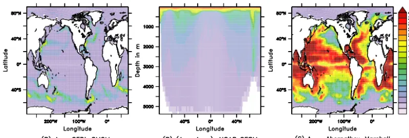
1/T =f/Ri1/2=f|dU/dz|/N≈ |Sρ|N, (5) where Sρ is the slope of density surfaces (Visbeck et al., 1997). In climate models, the slope is usually taken as some average slope over a range of depths (for example 100– 2000 m in Gnanadesikan et al., 2006). All else being equal, these approximations predict that growth rates and diffusion coefficients should be very small in the center of the subtrop-ical gyres where isopycnals are relatively flat. An example is shown in Fig. 2a for the GFDL CM2Mc model of Gal-braith et al. (2011). Because of its role in moving light tropi-cal waters into polar regions, particularly within the Southern Ocean,AGMhas a first-order impact on the large-scale
circu-lation of the ocean (Danabasoglu et al., 1994; Gnanadesikan, 1999). Values much larger than 1000 m2s−1in the main py-cnocline tend to produce unrealistic smoothing of the pycno-cline and suppression of the large-scale overturning circula-tion unless unrealistically high values of vertical mixing are applied in the tropics. Thus, in models whereARedi=AGM,
values applied in the center of subtropical gyres are often very low, on the order of a few hundred square meters per second.
MeasuringAGM directly from observations in nearly
im-possible, but several observational estimates ofARedido
ex-ist; these estimates seem incompatible with the values of
AGMdescribed above. Modern estimates ofARediusing a
va-riety of methods find relatively large values in the ocean interior. For example Ledwell et al. (1998), using SF6
re-leased into the thermocline, estimated an east–west diffusion of 1500 m2s−1 and a north–south diffusion of 600 m2s−1. Baynte et al. (2013), looking at the Guinea Dome, found a value of 1000–1200 m2s−1in the east–west direction and 500 m2s−1in the north–south direction. Estimates with sub-surface floats yield even larger values, with Bauer et al. (1998) estimating values of 2000–9000 m2s−1 in the equa-torial Pacific and Ollitraut and Colin de Verdiere (2002) finding values of 1500–3000 m2s−1 in the North Atlantic. A recently developed “pseudo-observational” approach uses satellite-derived surface geostrophic velocities to drive tracer or particle transport simulations (Shuckburgh and Haynes, 2003; Marshall et al., 2006; Shuckburgh et al., 2009; Rypina et al., 2012). Lateral diffusion coefficients can then be calcu-lated directly from such simulations. Abernathey and Mar-shall (2013) applied this method globally, producing the map of near-surfaceARedi shown in Fig. 2c. Finally, eddy
diffu-sion coefficients can be estimated from eddy-resolving nu-merical models (Abernathey et al., 2010; Fox-Kemper et al., 2012; Bachman et al., 2015). All these diverse estimates sug-gest thatARedi can be several times larger than the values
commonly used forAGM. This is the isopycnal mixing
para-dox.
One question is whether this paradox persists into the deep ocean. There are only a few direct estimates of ARedi
be-low the main thermocline. Ledwell and Watson (1991), in the Santa Barbara Basin, found a diffusion coefficient of 10– 20 m2s−1on spatial scales of 10 km. Rye et al. (2012) in the
Brazil Basin found a value of around 100 m2s−1. Both of
these, however, are at depths where lateral motion is likely to be strongly physically constrained by topography. There are no observational studies of which we are aware that directly estimate lateral diffusion between the base of the thermo-cline and depths associated with the tops of the mid-ocean ridges. In the few models where it is allowed to vary with depth,AGM is assumed to drop in the deep ocean, as eddy
kinetic energy is lower there. A zonal average ofAGM
illus-trating this is shown for the NCAR CESM model (Danaba-soglu et al., 2012) in Fig. 2b. However, if the surface values ofARedi are too low, forcing it to decrease with depth may
actually give less realistic deep values than the vast majority of parameterizations which simply prescribe values of 500– 1000 m2s−1uniformly throughout the water column.
Evalu-ating the extent to which this is the case is a major thrust of this paper.
Figure 2. Examples ofAGMandARedi. (a) Vertically uniformAGMfrom Galbraith et al. (2011). (b) Horizontal average ofARedi=AGM from Danabasoglu et al. (2012). (c) SurfaceARedifrom observationally based calculation of Abernathey and Marshall (2013).
diffusivities for both AGM and ARedi. Experiments are
on-going regarding the consequences of anisotropic eddy diffu-sion for ocean models (Reckinger and Fox-Kemper, 2015). It is not clear, however, how well the observational estimates capture the details of anisotropy, given that a particular chal-lenge in making such measurements is removing imperfectly known background shear flows (see for example LaCasce et al., 2014, who resolved this issue by looking at the cross-stream diffusivity only). Such shear flows may also cause tilts in the major and minor axes of the dispersion tensor that reflect resolved flows rather than details of the turbulence. Employing higher subgrid-scale diffusivities in the along-stream direction in models where one already resolves the large-scale flow may thus count the impact of the shear dis-persion twice.
Here, instead, we investigate another possible resolution: the non-equivalence between AGM and ARedi. Despite the
common assumption that they are equal, there is ample evidence that the two coefficients can differ significantly. Linear quasigeostrophic theory can be used to show that the diffusion coefficient governing lateral buoyancy trans-port (corresponding toAGM) is very different from the
co-efficient governing along-isopycnal PV (potential vorticity) transport, which is asymptotically equal toARedi(Smith and
Marshall, 2009; Vollmer and Eden, 2013). This theory has been tested in fully nonlinear primitive equation simulations (Abernathey et al., 2013). These studies all show ARedi to
be larger than AGM. Our experiments are designed to test
whether elevated values ofARedi throughout the water
col-umn give unrealistic results for helium isotopes and radio-carbon.
2.2 The helium–heat paradox
Given a decay of238U of 4.26 MeV=6.02×10⁻¹³J and a ra-tio ofR=3He/4He of 1.6×10⁻⁵as in Craig et al. (1975), we expect one mol year−1of3He to be associated with a global heat flux of about 800 MW. It is estimated that U decay contributes about 10–20 TW of heating, implying a flux of
around 12 500–25 000 mol3He year−1. However, Craig et al. (1975), using a box model calibrated with observations of
3He, estimated a much lower flux of 1070 mol year−1. This
has led to suggestions from geochemists that the mantle as a whole does not convect, so that helium is trapped in the deep mantle while heat escapes (O’Nions and Oxburgh, 1983). While alternative explanations for this difference have been proposed (see for example Harrison and Ballentine, 2003) the exact value of the mantle helium flux remains an important calibration point for geochemistry.
Box models are, however, a crude representation of the true rate at which the ocean is ventilated. As each box is rapidly homogenized, the effective transport of tracer from the deep ocean to the surface may be much larger than in the real world. This means that box models with the right mean overturning fluxes could overestimate the speed at which tracers make it out of the deep ocean, and thus would re-quire too large a source of 3He in the deep ocean. On the other hand, the neglect of mixing fluxes may mean that box models can underestimate the true flux.
Dutay et al. (2004) simulated helium isotopes in a suite of ocean general circulation models, which (presumably) have a more realistic representation of the processes that overturn the ocean. However, this paper found large ranges in the in-ventory of mantle helium. Given the differences in model construction it was far from clear why this was the case. Bianchi et al. (2010) revisited this problem using a suite of ocean-only models developed to look at the differing roles of vertical and lateral diffusion in setting global circulation. In these modelsAGM andARedi were varied together, with
Figure 3. Two box schematic of a tracer with a source (or sink) in the deep ocean, the signal of which is transported to the surface box by mass transportMoand equilibrated with the atmosphere by mass transportMa.
However, ifARedichanges are not directly tied to changes
inAGM, as may be the case in the real ocean, the picture is
potentially different. As shown in Pradal and Gnanadesikan (2014), increasingAReditends to destratify the high latitudes,
allowing more exchange with the deep ocean and causing sea ice to retreat. Thus, increasingARedi would be expected to
reduce mantle3He. The impact on radiocarbon is, however, less clear, given the long timescales involved in equilibration of carbon isotopes. An illustrative model of this is schema-tized in Fig. 3, in which a source of tracer is introduced into the deep box, circulation transports tracer between the inte-rior box and the surface box producing a fluxMo×(Cd−Cs)
and gas exchange restores the surface box to an equilibrium concentration with a flux Ma×(Cs−Ceq). At equilibrium,
both fluxes are equal toSand the deep concentration is just Cd=Ceq+S×(1/Mo+1/Ma) (6)
and similarly Cs=
Cd×Mo+Ceq×Ma
Mo+Ma
. (7)
Suppose (as we do) that the deep Pacific is primarily venti-lated from the Southern Ocean. For radiocarbon, the surface concentrations in the Southern Ocean are closer to the deep ocean mean of−170 ‰ than to zero, implying thatMois
ac-tually a little bigger thanMa(consistent with the idea that it
takes about 10 years to equilibrate the surface mixed layer). Thus, about half of the buildup of radiocarbon in the deep Pacific is due to slow gas exchange and will not be changed by increasing the ocean circulation. By contrast, helium iso-topes at the surface of the Southern Ocean are in equilibrium with the atmosphere, implying a much largerMa. This
im-plies that helium is more sensitive to changes in mixing than is radiocarbon. Could resolving the isopycnal mixing para-dox by breakingARedi andAGM apart result in a less
strin-gent helium–heat paradox as well? Or are changes in the ef-fective mixing rate over the range of potentialAReditoo small
to make a difference?
3 Model description and experimental setup
The physical climate model used here is described in Gal-braith et al. (2011) and is a lower-resolution version of the CM2M model of Dunne et al. (2012). The atmosphere has a horizontal resolution of 3.75◦×3◦ in the horizontal and has 24 levels in the vertical, with a topmost level at 3 mb and 4 layers in the bottom 100 mb to represent the surface boundary layer. The finite-volume core atmosphere model contains up-to-date parameterizations of gravity wave drag, clouds and radiation (the last of which has a diurnal cycle). The ocean has a nominal horizontal resolution of 3◦×2◦,
with enhanced zonal resolution near the Equator so as to re-solve the equatorial waveguide. In the vertical the resolution is 10 m over the top 100 m, increasing to 494 m at level 28, the bottom-most box. The ocean model is run withAGM
spa-tially varying as in Gnanadesikan et al. (2006) ranging be-tween 200 and 1400 m2s−1depending on the shear between 100 and 2000 m depth. AsAGM×Sdefines a streamfunction
for overturning that can become unrealistically large when slopes become infinite within the mixed layer, a maximum ofAGM×Smaxis applied withSmax=0.01. The coefficient
ARediby contrast is held fixed over time. For the control
ver-sion of the model a spatially constant value of 800 m2s−1 was used.
The model was initialized with modern ocean temper-atures and salinities and with greenhouse gasses and so-lar radiation fixed at 1860 levels. A 1500-year spinup was then performed, at which point three additional runs, with Aredi=400,1200, and 2400 m2s−1, were spun off the main
trunk and, along with the control, run for 1000 years. We will denote the runs by theARedi coefficient as AREDI400,
AREDI800, AREDI1200 and AREDI2400. Results are shown from the final century of these simulations.
An additional simulation, denoted ABER2D, sets ARedi
to the value calculated by Abernathey and Marshall (2013) for the surface layer that is shown in Fig. 2c. As is the case for all the other runs, this value is taken to be isotropic and depth-invariant. Neither assumption is likely to hold in the real world. The runs here should therefore be taken as a first step towards implementing a more realistic parameterization ofARedi. This simulation was also initialized from the
Additionally, simulations of mantle He based on the work of Dutay et al. (2004) were run. In the original protocol3He and4He are fixed in the atmosphere at prebomb levels and emitted from the ocean bottom along ridges. Following the work of Farley et al. (1995), injection is taken as propor-tional to the spreading rate and occurs at a depth approxi-mately 300 m above the ridge axis. In the original OCMIP2 (Ocean Carbon-Cycle Model Intercomparison Project Phase 2) protocol (Dutay et al., 2004) the total3He emission was normalized to give a global value of 1070 mol year−1(Craig et al., 1975) and no temperature anomaly was associated with the helium flux. Based on the work of Bianchi et al. (2010) this value was scaled down to 527 mol year−1. CM2Mc also includes a geothermal heat flux which varies from a value of around 50 mW m−2in the abyssal plains to peak values slightly above 100 mW m−2in the East Pacific Rise with a to-tal heat flux to the ocean of about 23TW. Both the bottom heat and He fluxes are held constant with time.
Spinup is an issue with coupled models. As described in Pradal and Gnanadesikan (2014) the surface temperatures are close to equilibrium after a few hundred years. This may not be the case for the deep ocean however, as the timescale for equilibrating radiocarbon can be many thousands of years, far longer than the spinups used in the majority of coupled climate models (which are generally from a few hundred to a few thousand years). Caution should thus be used in interpreting mean results. Since the models are initialized from observations, changes which enhance errors are likely to be significant, while it is possible that changes in diffusion which seem to reduce errors may in fact produce an over-shoot in the opposite direction after many thousands of years. The key metrics which we use here, in particular the relation-ships between helium and radiocarbon and the sharpness of the plumes, adjust much more rapidly, with a timescale of about 100 years. This can be seen by comparing the results in this version of the manuscript with the discussion paper, where results were presented after 500 years of simulation.
the differences at depth. The relative lack of sensitivity of the mean thermocline to changes inARedi stands in strong
contrast toAGM, which plays a major role in setting
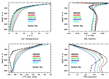
temper-atures at these depths (Danabasoglu et al., 1994; Gnanade-sikan, 1999). In the deep ocean, there is a general tendency for the models with higher levels of mixing to produce more realistic cold temperatures.
Salinity (Fig. 4b) shows a quite different behavior. The observed mean salinity profile is low at the ocean surface as a result of fresh mixed layers at high latitudes, it ex-hibits a subsurface maximum associated with the subtropi-cal gyres and a subsurface minimum associated with the for-mation of mode and intermediate waters. The lowest mix-ing case (AREDI400, black line) tends to overestimate the strength of polar haloclines, while the higher mixing cases (AREDI1200, AREDI2400 and ABER2D) all capture the near-surface salinity maximum while erasing vertical gradi-ents in salinity below about 1000 m. The AREDI800 simula-tion does a good job of capturing the deeper salinity structure but less of a good job near the surface. Together the temper-ature and salinity plots illustrate the difficulties in “tuning” Earth system models – parameterizations that improve one field may not improve another.
Radiocarbon (Fig. 4c) is generally too high in the mod-els, both at the surface and at depth. This suggests that ei-ther our rates of air–sea exchange, vertical exchange (due to advection and diffusion), or both are too vigorous. In gen-eral, increasing mixing tends to increase radiocarbon in the deep ocean, though the intramodel differences are gener-ally smaller than the model–observation differences. To first-order, the average depletion in the deep ocean is within about 15 ‰ of observations, implying an error in radiocarbon age of around 120 years.
Helium isotope anomalies (Fig. 4d) are also too large in the deep ocean (implying too little ventilation in contrast to ra-diocarbon). As expected, increasingAReditends to reduce the
Figure 4. Mean hydrography in the Earth system model suite. (a) Temperature, compared with the World Ocean Atlas. (b) Salinity compared with the World Ocean Atlas. (c) Radiocarbon, compared with Key et al. (2004). (d) Helium isotope anomaly compared with Bianchi et al. (2010).
4.2 Ventilation in the model suite
As discussed in Pradal and Gnanadesikan (2014), increas-ingARedi results in destabilizing the high-latitude Southern
Ocean and North Pacific. Models with more intense eddy mixing stir more salt into the high-latitude surface layer. This reduces the salinity contrast across the winter halo-cline, which is the dominant factor in determining vertical exchange in the subpolar North Pacific and Southern Ocean. The results of this can be seen in Fig. 5. The AREDI400 sim-ulation with the lowest mixing captures the value of the min-imum in radiocarbon in the North Pacific, though the depth at which this minimum is seen is too great. As ARedi
in-creases the result is to bring more young water down in the North Pacific, reducing the correlation between the observed and modeled zonal mean from 0.88 (AREDI400) to 0.71 (AREDI2400), and substantially increasing the RMSE (root mean squared error) in radiocarbon concentration from 22 (AREDI400) to 42 ‰ (AREDI2400). The Abernathey and Marshall (2013) spatially varying diffusion tends to act like low diffusion in the south, but higher diffusion in the north, and so also produces enhanced, unrealistic northern sink-ing, though not to the same extent as the AREDI2400 case. The differences between the AREDI400 and AREDI800 runs are largely due to an increase in the gradient between the Southern Ocean and the North Pacific, with the South-ern Ocean values of radiocarbon remaining relatively
un-changed, suggesting that lateral transport is important here. However, the differences between AREDI1200, AREDI2400 and AREDI800 show the impact of decreases in high-latitude stratification (particularly in the North Pacific) as well. In re-cent work (Gnanadesikan et al., 2015) we show that the de-stratification of the North Pacific also results in unrealistic uptake of anthropogenic carbon in this region.
Mantle helium shows a behavior somewhat similar to ra-diocarbon, but with the difference that the highest values are found in the tropical South Pacific rather than in the far north (Fig. 6a). The AREDI400 case largely captures the loca-tion of the maximum zonal meanδ3He anomaly but, as with radiocarbon, increasingARedi results in ventilation that
re-moves mantle helium from the far northern Pacific, decreas-ing the correlation with observations and raisdecreas-ing the mean error. There is, however, some sense that the lower values of ARedi result in an excessively high peak of mantle
Figure 5. Zonally averaged 114C (in ‰) in the Pacific. (a) From the observational data set of Key et al. (2004). (b) AREDI400. (c) AREDI800 (d) AREDI1200 (e) AREDI2400 (f) ABER2D.
4.3 Radiocarbon vs. mantle helium
The changes in deep tracers are reflected in changes in the scatterplot of deep δ3He vs. 114C (Fig. 7). As the mixing increases, the peak seen in the southeastern Pacific becomes smoothed out and the maximum depletion decreases. How-ever, all five runs lie close to the observed relationship. Since theδ3He values are linear in the source term, it is easy to see that doubling this term to the value of Craig et al. (1975) will lead to a strong offset. The results of Bianchi et al. (2010) appear to be robust against changes inARedi that are not
di-rectly associated with changes inAGM. Resolving the
isopy-cnal mixing paradox thus does not affect the helium–heat paradox.
This result is contrary to what might be expected from the changes in the tracers seen in Figs. 5 and 6, which show clear changes in the extreme values of these tracers in the deep ocean and substantially greater penetration of young waters asARediincreases. However, these changes in the endpoints
do not substantially change the effective rate at which tracer signals make their way from the deep ocean to the surface. Our results thus suggest that the key barrier to transfer be-tween the deep ocean and the surface is not mixing across the mixed layer base but transport from the ocean interior to the high-latitude regions. Such transport is accomplished both by advection and turbulent diffusion. If one considers a Péclet number for the deep South PacificU L/ARedi, deep
velocitiesUare on the order of 1 mm s−1but the length scale Lbetween where He is injected and where isopycnals reach the surface is on the order of 4000 km. Thus, even for the highest value of ARedi, the Péclet number is greater than 1
and advection dominates mixing.
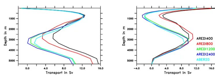
Examination of changes in overturning supports this idea. We can define the overturning as
Mover=
z2 Z z1 xe Z xw
v×dx×dz, (8)
wherevis the northward velocity, andxw, xe, z1andz2are
the limits of integration in the west, east, and vertical di-rections. The integral is taken at 30◦S in the Pacific. If the integral is performed relative to the surface (z1=z, z2=0,
Fig. 8a) the similarity in the northward transport of sur-face water is emphasized, but differences appear in the deep ocean. Note that the value does not go to zero at the bot-tom because water that flows into the southern Pacific leaves through the Indonesian throughflow and Bering straits. This net flux does change asARedi changes. Summing the
north-ward transport from the bottom of the ocean upnorth-ward (z1=
H, z2=zwhereH is the ocean depth, Fig. 8b), we see that
the models with constant ARedi all have similar inflows of
deep water of around 10 Sv (only the ABER2D simulation is noticeably lower). The main thing that changes between the simulations is whether this water is largely returned below the thermocline (as happens for the higher mixing cases) or
whether some small fraction of it upwells into the tropical thermocline and is returned through the Indonesian through-flow (as appears to be the case for AREDI400). From the point of view of flushing the deep tropical Pacific, however, it is largely irrelevant which pathway is taken. Instead, what matters is the throughflow, which is relatively constant across the different models.
4.4 The southeastern Pacificδ3He plume
Both the models and observations show high values in the southeastern Pacific, where a rapidly spreading rift releases large amounts of mantle helium. The sharpness of this plume, however, varies substantially between the models. In Fig. 9, the distributions at 2500 m are overlaid with the actual ob-servations between 2250 and 2750 m (filled squares). Differ-ences in color thus highlight locations where the model is mismatched with the in situ observations. In Fig. 9a we see that there are some differences between the gridded and in situ observations. This reflects the fact that in order to ex-trapolate over the relatively coarse observations in the deep ocean to a global data set, Bianchi et al. (2010) had to de-fine a radius of influence that effectively smooths the data and may be comparable to the size of some of the features seen in the model output. For this reason, we have not cho-sen to precho-sent RMSEs, as these would imply a greater degree of precision than is justified given the coarseness of the sam-pling and the model.
However, even a qualitative comparison makes it clear that the mixing exerts a strong control over how well the models match the observations. In the AREDI400 run (Fig. 9b), the symbols over the East Pacific Rise show up as lower than the model, which produces a peak value exceeding 70 %, while the highest values in the observations are around 45 %. By contrast, the AREDI2400 model produces no values higher than 36 %. The AREDI800, AREDI1200 and ABER2D mod-els all produce peaks that are qualitatively similar to obser-vations.
This is not merely the impact of the depth chosen. Fig-ure 10 shows a depth–longitude section of δ3He cutting through the center of the plume between latitudes of 20 and 30◦S. Again, we see that the observations over the ridge show up as too low in the AREDI400 run, too high in the AREDI2400 run and close to the simulated values for the AREDI800, AREDI1200 and ABER2D simulations (though note that the highest values in the models are displaced down-wards relative to observations). This suggests that very low diffusion coefficients in the deep southeastern Pacific are not consistent with the release of helium there, in contrast to cur-rent theory. The values that are most consistent with the ob-servations are comparable to what is found nearer to the sur-face. This suggests that the isopycnal mixing paradox is not simply a matter ofARedi being much larger thanAGMin the
Figure 7. Scatterplots of δ3He vs.114C for different values ofARedi. On all plots observations are in black. (a) AREDI400 (red) and AREDI800 (blue). (b) AREDI1200 (red) and AREDI2400 (blue) (c) ABER2D (red).
Figure 8. Overturning in the South Pacific at a latitude of 30◦S across the different model runs. Overturning is computed as a running sum of northward transport. (a) Overturning summed from top to bottom, emphasizing similarity in northward surface flow. (b) Overturning summed from bottom to top, emphasizing similarity in deep inflow of Antarctic Bottom Water.
5 Conclusions
Our simulations of helium isotopes and radiocarbon have not resolved either of the two paradoxes outlined earlier in the paper. While larger values of isopycnal mixing varying in-dependently of AGM do allow for more exchange between
the surface and deep ocean, this exchange does not change the fundamental relationship between radiocarbon and he-lium isotopes in the deep ocean. Isopycnal mixing does not offer a solution to the helium paradox. Moreover, the distri-bution of helium isotopes in the abyssal ocean do not sup-port the idea that values ofARedibelow the thermocline must
be much smaller than values at the surface, as found in the NCAR CESM model. Nor do they support the idea that the coefficients must be much smaller than the values of AGM
found in boundary currents where isopycnal slopes are much larger, as found in models such as GFDL’s ESM2G. Instead, relatively large values ofARedi are needed to produce
suffi-ciently diffuse plumes.
Resolving the helium paradox is beyond both the scope of this paper and the expertise of the authors. However, we can comment on the isopycnal mixing paradox. Recall that this
paradox stems from three assumptions – equivalence ofAGM
andARedi, a strong relationship betweenAGMand
baroclin-icity, and limits on the maximum value ofAGM. While the
last two of these appear to be well founded in theory and modeling, it is not at all clear thatAGMshould equalARedi.
Indeed, recently published estimates ofAGMandARedibased
on theory (Smith and Marshall, 2009; Vollmer and Eden, 2013) and simulation (Abernathey et al., 2013) show differ-ent values for the two coefficidiffer-ents. Our results here support the idea that breaking this equivalence allows for more re-alistic tracer distributions in many parts of the ocean, par-ticularly in the abyssal South Pacific. The reasons why this equivalence breaks down are less clear but likely have to do with the fact that anomalies in layer height can be tightly connected to anomalies in velocity, and that viscous forces act to smooth out such variations in ways that they do not act to smooth out variations in passive tracers.
er-Figure 9.δ3He (in %) in the SE Pacific between the depths of 2250 and 2750 m. Symbols are taken from observational data set of Bianchi et al. (2010). (a) Gridded data set of Bianchi et al. (2010) showing effects of smoothing. (b) AREDI400. (c) AREDI800. (d) AREDI1200. (e) AREDI2400. (f) ABER2D.
ers, however, requires knowledge about sources and sinks that are not always well-constrained. We suggest that more attention to tracer–tracer relationships, particularly regarding radiocarbon, may be helpful in this regard.
While the results here do support the idea that the isopyc-nal mixing paradox should be resolved in favor of allowing ARedi to differ fromAGM and indicate that relatively large
values ofARedi in the ocean interior do not result in
break-ing the models, more work is clearly needed to find a fully prognostic parameterization. Three areas in particular require more attention.
1. Because coupled models do not necessarily place boundary currents in the right place, fixingARedias we
have done here can result in higher impacts of isopycnal mixing in boundary currents than is physically reason-able. This may be one reason that the ABER2D simula-tion produces too much convecsimula-tion in the North Pacific. Our results support the continued development of mod-els that predict both the length and timescales involved in isopycnal mixing.
2. Our ABER2D results assumed a mixing coefficient that is isotropic. In reality, mixing is probably larger in the zonal or along-flow direction than in the meridional or cross-flow direction. Better constraining of anisotropy in both observations and numerical simulations remains an important task.
3. Our results also assume that ARedi is constant with
depth. Again, both numerical simulations (Abernathey et al., 2013) and limited observational results (Rye et al., 2012) suggest this is unlikely to be the case, with higher values at internal critical layers and lower values in the deep ocean where flow is constrained by topography. More work is needed however, to constrain this vertical dependence, as our results suggest it is unlikely to be simply related to stratification.
The Supplement related to this article is available online at doi:10.5194/os-11-591-2015-supplement.
Abernathey, R. and Marshall, J.: Global surface eddy diffusivities derived from satellite altimetry, J. Geophys. Res.-Oceans, 118, 901–916, 2013.
Abernathey, R., Marshall, J., Shuckburgh, E., and Mazloff, M.: En-hancement of mesoscale eddy stirring at steering levels in the Southern Ocean, J. Phys. Oceanogr., 40, 170–185, 2010. Abernathey, R., Ferreira, D., and Klocker, A.: Diagnostics of
isopy-cnal mixing in a circumpolar channel, Ocean Model., 72, 1–16, 2013.
Anderson, D.: The helium paradoxes, P. Natl. Acad. Sci. USA, 95, 4822–4827, 1998.
Bachman, S., Fox-Kemper, B., and Bryan, F. C.: A tracer-based inversion method for diagnosing eddy-induced diffusivity and advection. Ocean Model., 86, 1–14, doi:10.1016/j.ocemod.2014.11.006, 2015.
Bauer, S., Swenson, M. S., Griffa, A., Mariano, A. J., and Owens, K.: Eddy-mean flow decomposition and eddy-diffusivity estimates in the tropical Pacific Ocean, 1. Methodology, J. Geo-phys. Res., 103, 30855–30871. 1998.
Baynte, D., Visbeck, M., Tanhua, T., Krahmann, G., and Karstensen, J.: Lateral diffusivity from tracer release experiments in the tropical thermocline, J. Geophys. Res.-Oceans, 118, 2719– 2733, 2013.
Bentsen, M., Bethke, I., Debernard, J. B., Iversen, T., Kirkevåg, A., Seland, Ø., Drange, H., Roelandt, C., Seierstad, I. A., Hoose, C., and Kristjánsson, J. E.: The Norwegian Earth System Model, NorESM1-M – Part 1: Description and basic evaluation of the physical climate, Geosci. Model Dev., 6, 687–720, doi:10.5194/gmd-6-687-2013, 2013.
Bianchi, D., Sarmiento, J. L., Gnanadesikan, A., Key, R. M., Schlosser, P., and Newton, R.: Low helium flux from the mantle inferred from simulations of oceanic helium isotope data, Earth Planet. Sc. Lett., 297, 379–386, doi:10.1016/j.epsl.2010.06.037, 2010.
Craig, H., Clarke, W. B., and Beg, M. A.: Excess3He in deep wa-ter on the East Pacific rise, Earth Planet. Sc. Lett., 26, 125–132, 1975.
Danabasoglu, G., McWilliams, J. C., and Gent, P.: The role of mesoscale tracer transports in the global ocean circulation, Sci-ence, 264, 1123–1126, 1994.
Danabasoglu, G., Bates, S. C., Brieglieb, B. P., Jayne, S. R., Jochum, M., Large, W. G., Peacock, S., and Yeager, S. G.: The CCSM4 ocean component, J. Climate, 25, 1361–1389, 2012. Dunne, J. P., John, J. G., Adcroft, A. J., Griffies, S. M.,
Sentman, L. A., Samuels, B. L., Spelman, M. J., Win-ton, M.,Wittenberg, A. T., and Zadeh, N.: GFDL’s ESM2 global coupled climate-carbon Earth System Models Part I: Physical formulation and baseline simulation characteristics, J. Climate, 25, 6646–6665, 2012.
Dutay, J.-C., Jean-Baptiste, P., Campin, J.-M., Ishida, A., Maier-Reimer, E., Matear, R. J., Mouchet, A., Totterdell, I. J., Ya-manaka, Y., Rodgers, K., Madec, G., and Orr, J. C.: Evaluation of OCMIP-2 ocean models’ deep circulation with mantle helium-3, J. Marine Syst., 48, 15–36, 2004.
Eady, E.: Long waves and cyclone waves, Tellus, 1, 33–52, 1949. Emerson, S. and Hedges, J. I.: Chemical Oceanography and the
Ma-rine Carbon Cycle, Cambridge Univ. Press, New York, 2008. Farley, K. A., Maier-Reimer, E., Schlosser, P., and Broecker, W. S.:
Constraints on mantle He-3 fluxes and deep-sea circulation from an ocean general circulation model, J. Geophys. Res., 100, 3829– 3839, 1995.
Fogli, P., Manzini, E., Vichi, M., Alessandri, A., Patara, L., Gualdi, S., Scoccimoarro, E., Masina, S., and Navarra, A.: INGV-CMCC Carbon (ICC): a carbon cycle earth system model, Tech-nical Rep. 61, Centro Euro-Mediterraneo per i Cambiamenti Cli-matici, Bologna, 2009.
Fox-Kemper, B, Lumpkin, R., and Bryan, F. O.: Lateral transport in the ocean interior, in: Ocean Circulation and Climate – Ob-serving and Modelling the Global Ocean, edited by: Siedler, G., Church, J., Gould, J., and Griffies, S., Elsevier, New York, 2012. Galbraith, E. D., Gnanadesikan, A., Dunne, J. P., and His-cock, M. R.: Regional impacts of iron-light colimitation in a global biogeochemical model, Biogeosciences, 7, 1043–1064, doi:10.5194/bg-7-1043-2010, 2010.
Galbraith, E. D., Kwon, E.-Y., Gnanadesikan, A., Rodgers, K. B., Griffies, S. M., Bianchi, D., Dunne, J. P., Sarmiento, J. L., Simeon, J., Slater, R. D., Wittenberg, A. T., and Held, I. M.: Climate variability and radiocarbon in the CM2Mc Earth System Model, J. Climate, 24, 4230–4254, doi:10.1175/2011JCLI3919.1, 2011.
Gent, P. and McWilliams, J. C.: Isopycnal mixing in ocean mod-els, J. Phys. Oceanogr., 20, 150–155, 1990.
Gnanadesikan, A.: A simple model for the structure of the oceanic pycnocline, Science, 283, 2077–2079, 1999.
Gnanadesikan, A., Dixon, K. W., Griffies, S. M., Balaji, V., Barreiro, M, Beesley, J. A., Cooke, W. F., Delworth, T. L., Gerdes, R., Harrison, M. J., Held, I., Hurlin, W. J., Lee, H. C., Liang, Z., Nong, G., Pacanowski, R. C., Rosati, A., Russell, J. L., Samuels, B. L., Song, Q., Spelman, M. J., Stouffer, R. J., Sweeney, C., Vecchi, G. A., Winton, M., Wittenberg, A. T., Zeng, F., Zhang, R., and Dunne, J. P.: GFDL’s CM2 Global cou-pled climate models: Part II: The baseline ocean simulation, J. Climate, 19, 675–697, 2006.
Gnanadesikan, A., Bianchi, D., and Pradal, M. A.: Critical role for mesoscale eddy diffusion in supplying oxygen to hy-poxic ocean waters, Geophys. Res. Lett., 40, 5194–5198, doi:10.1002/grl.50998, 2013.
Gnanadesikan, A., Pradal, M. A., and Abernathey, R. P.: Isopyc-nal mixing by mesoscale eddies significantly impacts oceanic an-thropogenic carbon uptake, Geophys. Res. Lett., 42, 4249–4255, doi:10.1002/2015GL064100, 2015.
Gordon, J., O’Farrell, S., Collier, M., Dix, M., and Rotstayn, L., Kowalczyk, Hirst, T., and Watterson, I.: The CSIRO Mk3.5
Cli-mate model, Tech. Rep. 21, Center for Australian Weather and Climate Research, Melbourne, 2010.
Green, J. S.: Transfer properties of the large-scale eddies and the general circulation of the atmosphere, Q. J. Roy. Meteor. Soc., 96, 157–185, 1970.
Griffies, S. M.: The Gent–McWilliams skew flux, J. Phys. Oceanogr., 28, 831–841, 1998.
Griffies, S. M., Gnanadesikan, A., Pacanowski, R. C., Larichev, V. D., Dukowicz, J. K., and Smith, R. D.: Isoneutral diffusion in az-coordinate ocean model, J. Phys. Oceanogr., 28, 805–830, 1998.
Harrison, D. and Ballentine, C. J.: Noble gas models of mantle structure and reservoir mass transfer, Earth’s Deep Mantle: struc-ture, composition and evolution, Geophys. Monogr. Ser., 160, 9– 26, 2003.
Jones, C. D., Hughes, J. K., Bellouin, N., Hardiman, S. C., Jones, G. S., Knight, J., Liddicoat, S., O’Connor, F. M., An-dres, R. J., Bell, C., Boo, K.-O., Bozzo, A., Butchart, N., Cad-ule, P., Corbin, K. D., Doutriaux-Boucher, M., Friedlingstein, P., Gornall, J., Gray, L., Halloran, P. R., Hurtt, G., Ingram, W. J., Lamarque, J.-F., Law, R. M., Meinshausen, M., Osprey, S., Palin, E. J., Parsons Chini, L., Raddatz, T., Sanderson, M. G., Sellar, A. A., Schurer, A., Valdes, P., Wood, N., Woodward, S., Yoshioka, M., and Zerroukat, M.: The HadGEM2-ES implemen-tation of CMIP5 centennial simulations, Geosci. Model Dev., 4, 543–570, doi:10.5194/gmd-4-543-2011, 2011.
Key, R. M., Kozyr, A., Sabine, C. L., Lee, K., Wan-ninkhof, R., Bullister, J., Feely, R. A., Millero, F., Mordy, C., and Peng. T.-H.: A global ocean carbon climatology: re-sults from GLODAP, Global Biogeochem. Cy., 18, GB4031, doi:10.1029/2004GB002247, 2004.
Khatiawala, S., Primeau, F., and Holzer, M.: Ventilation of the deep ocean constrained with tracer observations and implications for radiocarbon estimates of ideal mean age, Earth Planet. Sc. Lett., 325–326, 116–125, doi:10.1016/j.epsl.2012.01.038, 2012. Ledwell, J. R. and Watson, A. J.: The Santa Monica Basin tracer
ex-periment: a study of diapycnal and isopycnal mixing, J. Geophys. Res., 103, 214999–215129, 1991.
Ledwell, J. R., Watson, A. J., and Law, C. S.: Mixing of a tracer in the pycnocline, J. Geophys. Res., 103, 21499–21529, 1998. Marshall, J., Shuckburgh, E., Jones, H., and Hill, C.: Estimates and
implications of surface eddy diffusivity in the Southern Ocean derived from tracer transport, J. Phys. Oceanogr., 36, 1806–1821, 2006.
Ollitraut, M. and Colin de Verdiere, A.: SOFAR floats reveal mid-latitude intermediate North Atlantic circulation, Part II: An Eu-lerian statistical view, J. Phys. Oceanogr., 32, 2034–2053, 2002. O’Nions, R. K. and Oxburgh, E. R.: Heat and helium in the earth,
Nature, 306, 429–431, 1983.
Pradal, M.-A. and Gnanadesikan, A.: Impact of isopycnal stirring on global climate in an Earth System Model, J. Adv. Model. Earth Sys., 6, 586–601, doi:10.1002/2013MS000273, 2014. Reckinger, S. J. and Fox-Kemper, B.: Anisotropic mesoscale eddy
transport in ocean general circulation models, in preparation, 2015.
Redi, M. H.: Ocean isopycnal mixing by coordinate rotation, J. Phys. Oceanogr., 12, 1154–1157, 1982.
using a tracer-based coordinate system, Phys. Fluids, 15, 3342– 3357, 2003.
Shuckburgh, E., Jones, H., Marshall, J., and Hill, C.: Robust-ness of effective diffusivity diagnostic in oceanic flows, J. Phys. Oceanogr., 39, 1993–2009, 2009.