Continuous dynamic assimilation of the inner region data in hydrodynamics modelling: optimization approach

(1)

www.nonlin-processes-geophys.net/15/815/2008/ © Author(s) 2008. This work is distributed under the Creative Commons Attribution 3.0 License.

Nonlinear Processes

in Geophysics

Continuous dynamic assimilation of the inner region data in

hydrodynamics modelling: optimization approach

F. I. Pisnitchenko1, I. A. Pisnichenko2, J. M. Mart´ınez1, and S. A. Santos1 1_{State University of Campinas, Campinas, SP, Brazil}

2_{Center for Weather Forecast and Climate Studies/National Inst. for Space Research – INPE, Cachoeira Paulista, SP, Brazil} Received: 22 February 2008 – Revised: 30 May 2008 – Accepted: 9 September 2008 – Published: 3 November 2008

Abstract. In meteorological and oceanological studies the classical approach for finding the numerical solution of the regional model consists in formulating and solving a Cauchy-Dirichlet problem. The boundary conditions are obtained by linear interpolation of coarse-grid data provided by a global model. Errors in boundary conditions due to interpolation may cause large deviations from the correct regional solu-tion. The methods developed to reduce these errors deal with continuous dynamic assimilation of known global data avail-able inside the regional domain. One of the approaches of this assimilation procedure performs a nudging of large-scale components of regional model solution to large-scale global data components by introducing relaxation forcing terms into the regional model equations. As a result, the obtained solu-tion is not a valid numerical solusolu-tion to the original regional model. Another approach is the use a four-dimensional vari-ational data assimilation procedure which is free from the above-mentioned shortcoming. In this work we formulate the joint problem of finding the regional model solution and data assimilation as a PDE-constrained optimization prob-lem. Three simple model examples (ODE Burgers tion, Rossby-Oboukhov equation, Korteweg-de Vries equa-tion) are considered in this paper. Numerical experiments indicate that the optimization approach can significantly im-prove the precision of the regional solution.

1 Introduction

Studying and modelling different physical processes fre-quently require to solve Cauchy-Dirichlet problems. In geophysical investigations, for solving the Cauchy-Dirichlet

Correspondence to: F. I. Pisnitchenko ([email protected])

problem, numerical methods are usually employed. The dis-crete form of equations and initial and boundary values at the points of the grid are traditionally used in these meth-ods. The problem is generally solved by means of a proper numerical scheme. However, both initial and boundary val-ues, which are obtained from measurements or other model outputs, contain errors, which can reach 30% from the true values.

For some problems, the solution can be very sensitive to these errors. On the other hand, some values of the sought solution at some points of the inner region, along with ini-tial and boundary data, are often available. Of course, these additional data also have errors. The question arises: is it possible to improve the accuracy of the model solution of the Cauchy-Dirichlet problem by using these additional data? For some well-known equations of mathematical physics and dynamic meteorology we will show here that the use of ad-ditional information on the solution values within the inte-gration region can noticeably improve the accuracy of the solution.

(2)

period of more than 3 h and space scale larger than 60 km. Regional models can simulate the evolution of mesometeo-rological fast processes (small cyclones, storms, tornados), with time period of less than 3 h and spatial extent between 2 and 60 km.

These models are described mathematically by systems of nonlinear partial differential equations. To solve the system corresponding to a global model we need only the initial con-dition and bottom and upper boundary concon-ditions, since the domain is the whole sphere. To get the solution of a sys-tem corresponding to a regional model we also need lateral boundary conditions. The lateral boundary conditions for a regional model are obtained from the global model using in-terpolation. These conditions do not provide information on the structures of the scales smaller than the size of the mesh of the global model. In fact, global models do not distinguish a local meteorological phenomenon of characteristic length scale smaller than 30 km, because the space step is greater than this value. On the other hand, the parts of space and time spectrums of a regional model solution which correspond to large-scale structures and long-period processes are in worse accordance with observations than those of a global model. This is related to the fact that a regional model does not have the information about the phenomena that occur outside its domain.

For example, the weakly regular, low frequency oscilla-tions of the sea surface temperature of tropical Pacific in central part and near the Peru coast, known as El Niño and La Niña events, have a large influence on the climate of the tropical and subtropical regions. The circulation regimes in these regions noticeably differ during these events. Re-gional models, driven, for example, by the Reanalysis data, do not reproduce with confidence this distinction between the El Niño and La Niña regimes (Seth et al., 2007; Gershunov et al., 2000). The reason of this inconsistency is, probably, poor space and time data resolution on the regional model boundaries. Mathematically, this means that the solution of this boundary value problem is strongly sensitive to errors on the boundaries (Denis, Laprise and Caya, 2003; Diaconescu, Laprise and Sushama, 2007).

The spectral nudging technique is one of methods pro-posed to use additional data from the inner domain in or-der to reduce boundary error influence and to improve the solution of an initial-boundary value problem (Waldron et al., 1996; Storch et al., 2000; Kanamaru and Kanamitsu, 2005). This method supposes incorporation of the largest internal modes of some meteorological variables from ob-servations or from a driving model into the regional model solution. However, the use of the spectral nudging tech-nique requires inserting additional forcing terms into the evolution equations of a regional model. Hence, the original model is corrupted and its new solution may not be close to the correct regional solution.

Another method which is aims to avoid strong sensitivity of regional model solution with respect to the boundary con-dition errors is based on four-dimensional variational (4D-Var) data assimilation procedures (Le Dimet and Talagrand, 1986; Rabier, 2005; Lorenc and Payne, 2007). In the papers of Leredde et al. (1998), Zou and Kuo (1996), Lu and Brown-ing (2000) and Griffin and Thomson (1996) optimization ap-proach is applyed to restore boundary conditions using data within spatial model domain. 4D-Var performs an adjust-ment of the model trajectory with all available data (obser-vations or global model data) taken explicitly at the precise time and thus the obtained model solution is maximally pos-sibly consistent with available observations.

In this work we apply the optimization theory to the 4D-Var data assimilation procedure. Firstly, in Sect. 2 we give the formulation of the Cauchy-Dirichlet problem for a re-gional model and the general formulation of an optimization problem, and we show how the latter (with the accessibility of some additional conditions) can be applied for finding the solution of the former. In Sect. 3, for some simple equations, we show how the optimization approach can be used to ob-tain a solution of the initial boundary value problem. The equations considered here include the ordinary differential equation of Burgers, the one-dimensional linearized Rossby-Oboukhov partial differential equation, and the partial differ-ential equation of Korteweg – de Vries. We also compared the sensitivity of the solutions, obtained by the traditional and the new approach with respect to the errors in the bound-ary conditions. In Sect. 4 we discuss the obtained results. Appendix A provides more detailed description of the opti-mization procedure.

2 Numerical solution of regional problems

2.1 Classical approach

We formulate here the Cauchy-Dirichlet problem as it is stated for regional weather forecast. To find a unique so-lution for the regional model equations we need the lateral boundary condition for the entire time interval on which the solution is required. Usually, these data are obtained from the solution of an outer (global) model. We do not know the exact solution of the outer model (otherwise, our problem would have been already solved), but we can find its approx-imate solution in the discrete form:

1t{9}=Fd,

9(x,0)=Yglobal(x), 9(x, t )|_x∈B =9b(x, t ).

(1)

Here1t is the evolution operator of the discrete model, 9

is the vector of the prognostic functions, Fd are discrete

(3)

5 5.5 6 6.5 7 7.5 8 8.5 9 9.5 10 8

10 12 14 16 18 20 22 24 26

x

y

exact solution observations classical aproach

Fig. 1. Solution ofy00=0 using classical approach.

lower (and maybe lateral) boundaries of the global model, and9bis the boundary condition. Let9solbe the solution of

(1). It is supposed that this solution is sufficiently close to the solution of hypothetical ideal model which exactly describes the real atmospheric processes.

The regional model is located in a closed area with bound-ary S and its discrete representation can be written in the same manner as for the global model:

δt{G}=Frd,

G(x,0)=Ylocal(x), G(x, t )|_x_∈_S=Gs(x, t ),

(2)

whereδt is the evolution operator of the discrete regional

model,Gis the vector of the prognostic functions andFrd

are discrete external forces,Ylocalis the initial condition, and Gsis the boundary condition.

The traditional approach to seek the solution of (2) con-sists in the interpolation of required data from 9sol on the regional grid for forming the boundary and initial condi-tions, and then applying any numerical method to solve the model equations. However, as we have mentioned above, the boundary conditions contain errors which can strongly cor-rupt the solution.

The use of the information obtained from the solution of the global model equations9sol on the values inside the re-gional model domain for all available time moments can help to overcome this difficulty.

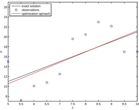
5 5.5 6 6.5 7 7.5 8 8.5 9 9.5 10 8

10 12 14 16 18 20 22 24 26

x

y

exact solution observations optimization aproach

Fig. 2. Solution ofy00=0 using optimization approach.

2.2 Optimization approach

As mentioned in the previous section, in the classical ap-proach we obtain the boundary conditions for the regional model by means of interpolation of the coarse grid solution provided by the global model. Essentially, interior points also provided by the global model are discarded. The op-timization approach consists of taking not only close-to-the boundary points on the global grid, but also global solu-tion values at interior points. A trivial example will clar-ify this procedure and show its plausibility. Assume that (x1, y1), . . ., (xm, ym)are “global model” observations and

that we want to fit the “local model” defined byy00=0. The “classical approach” would consist in taking, as solution, the line that joins (x1, y1) with (xm, ym). The optimization

ap-proach consists in finding the regression line that considers all the points. If the data were free of errors, both results would be identical, but, in the presence of errors, the differ-ence may be dramatic. In Figs. 1 and 2 we show an example where the data (xi, yi+ei),i=1, . . ., m, corresponding to the

exact solutiony=2x+1, were randomly perturbed, whereei

represents a±30% ofyi. It is easy to see that only the

op-timization approach provides a reasonably accurate solution. We claim that the same situation occurs in more complicate mathematical environments.

The required solution of the regional model must satisfy the regional-model differential equations and the observed initial conditions. Therefore, the regional model solution must satisfy the constraints

δt{G}−Frd=0

(4)

Among the set of functions that satisfy these constraints we seek the one that minimizes the distance to the observed points9sol produced by the global model. Therefore, we have the optimization problem:

Minimized(G, 9sol) subject to (s.t.)δt{G}−Frd=0,

G(x,0)−Ylocal(x)=0.

(4)

Hered(:,:)is the objective function, which represents the distance betweenG and9sol. In other words, we want to minimize the distance between the regional and the global model solutions under constraints that say that the regional model equations and the initial condition are satisfied. Note here that, when we talk about the solutionG, we bear in mind the vectorG=G(x, t )in a grid space of (x, t) – coordinates, wheret corresponds to discrete time points of the regional model integration andx to discrete mesh points in the re-gional model area.

For a long integration time, the dimension of the mini-mization problem can become too large, making it imposible to be solved. Then, instead of solving it as a unique prob-lem, we split it in several minimization problems as follows. The time is divided in periods and, for each period, the re-lated minimization problem has an appropriate dimension. The model is solved by means of the minimization problem in each period. For the first problem, the initial condition is taken from the “observations”. For the second problem, the initial condition is the solution of the previous problem (first problem) in the lastest time level. And so on the minimiza-tion problems are solved until the last period.

The use of optimization algorithms for analysis and assim-ilation in meteorology has been considered by many authors. Modern optimization approach methods were discussed in the survey of Rabier (2005). One of the first and fundamen-tal papers which placed the basis of application of optimiza-tion theory to meteorology and presented some algorithms for the realization of this method is the paper of Le Dimet and Talagrand (1986). This paper also includes detailed ref-erences on the previous works. The general idea of opti-mization approach is, always, to find the solution of a given model which is closest to a set of “observations”. In our case, the “observations” must be interpreted as the solution of the global model. In (Le Dimet and Talagrand, 1986) the authors discuss, among other methods, the use of the Aug-mented Lagrangian methodology for solving the associated minimization problem. By means of Augmented Lagrangian methods the original problem is solved as a sequence of un-constrained optimization problems where the objective func-tion includes informafunc-tion on the constraints. This approach is very adequate in general optimization for large scale prob-lems in which the Jacobian information is badly structured,

so that sparse matrix techniques for solving linear systems are hard to employ. The main disadvantage of the Aug-mented Lagrangian method is that the final convergence speed uses to be poor, although acceleration techniques have been recently introduced (?Birgin and Mart´ınez, 2008). However, acceleration techniques are based on the direct consideration of the optimality (Euler-Lagrange) conditions of the system, and may be used in the cases in which sparsity can be handled. In many optimization problems the Euler-Lagrange nonlinear system is suitably structured and can be solved by means of Newtonian or quase-Newton techniques (Mart´ınez, 2000). As a matter of fact, our first attack to the problems reported in this paper was by means of the Aug-mented Lagrangian, using the modern software Algencan (Andreani et al., 2007, 2008) In spite of being successful in obtaining solutions, we found that computer time was unac-ceptable and, so, we switched to the Newtonian technique.

(5)

3 Examples of application of the optimization method to the problems of small dimension

3.1 Burgers’ equation

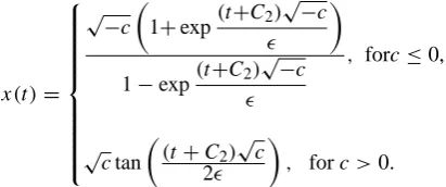
We will exhibit an application of the optimization method to problems of small dimension. As a first example we consider the supersensitive boundary value problem for the Burgers’ equation (Boh´e, 1996), used for describing wave processes in acoustics and hydrodynamics:

x00= −xx0,

x(0)= −1, x(T )=1, (5)

wherexis velocity andis the viscosity coefficient. To get the analytical solution of this problem it is enough to integrate the left and right sides of the Eq. (5) overt:

x0= −x

2₊_c 2 .

Then, after rewriting the foregoing formula as dx

x2₊_c= − dt

2

and integrating the left side overx and the right one overt, we can write the Burgers’ equation solution as

x(t )=

         

        

√ −c

1+exp(t+C2)

√ −c

1−exp(t+C2)

√ −c

, forc≤0,

√

ctan

(t+C2)

√

c 2

, forc >0.

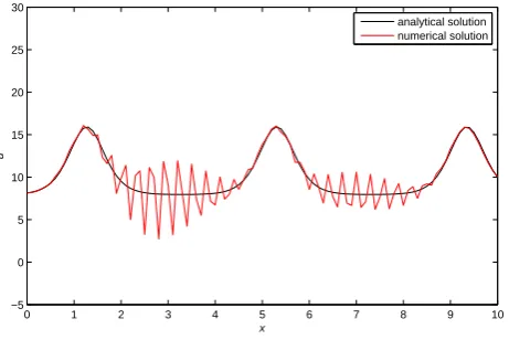
The graph of the analytical solution for Eq. (5) with the boundary condition x(0)= −1, x(1)=1 and =0.05 is pre-sented in Fig. 3 (black line).

Let us choose several points from the analytical solution and slightly perturb them (till 5% from its real value). This procedure models the boundary and inner domain data con-taining errors. Using these perturbed data for the boundary pointsx(0),x(1)we solve the boundary problem (5) apply-ing the shootapply-ing method. For the step1t=0.01 the numerical solution is presented in Fig. 3 by red line.

As one can see, small perturbations of the boundary condi-tion result in large errors in the solucondi-tion. Now, let us solve the problem using optimization formulation (4) with additional information about the perturbed solution on the points in-side the domain, conin-sidering the same discretization as when solving (5) by the traditional shooting method, with the same 1t=0.01.

0 0.1 0.2 0.3 0.4 0.5 0.6 0.7 0.8 0.9 1 −1.5

−1 −0.5 0 0.5 1 1.5

t

x

analitical solution boundary condition numerical solution

Fig. 3. Analitical solution (black line), usingx(0)=−1,x(1)=1 as

boundary condition, and numerical solution (red line), using 5% perturbed boundary condition (circles), of Burgers’ equation.

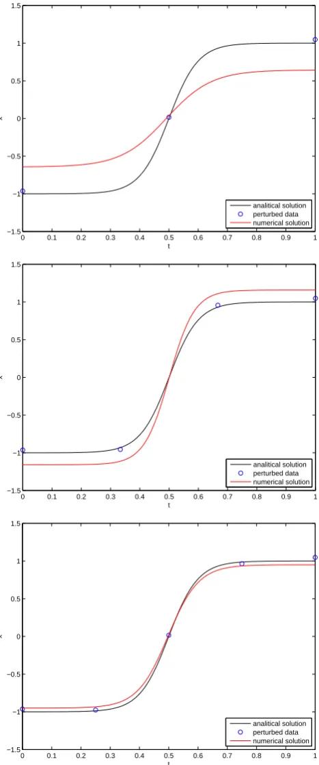
Figure 4 shows the solutions of the optimization problem for the three cases when we used 3, 4 and 5 points of the perturbed solution, respectively. One can see that all these solutions correspond better to the analytical one, than the so-lution obtained by the traditional approach. In the case of using the three additional inner points, the optimization solu-tion and the analytical solusolu-tion almost coincide. This exam-ple shows that there are dynamical systems in which small perturbations (≤5%) in the boundary conditions can lead to great errors in the final solution. However, if some additional information exists, that information can be used to improve significantly the solution, applying optimization.

3.2 Rossby-Oboukhov one-dimensional equation

The two-dimensonal non-linear Rossby-Oboukhov equation describes the evolution of potential vorticity in barotropic at-mosphere (Oboukhov, 1949). In this example we consider the one-dimensional linear equation obtained during the lin-earization procedure of the Rossby-Oboukhov equation.

∂ ∂t

∂2 ∂x2−

1 l₀2

!

ψ+β∂ψ ∂x+U

∂3ψ

(6)

0 0.1 0.2 0.3 0.4 0.5 0.6 0.7 0.8 0.9 1 −1.5

−1 −0.5 0 0.5 1 1.5

t

x

analitical solution perturbed data numerical solution

0 0.1 0.2 0.3 0.4 0.5 0.6 0.7 0.8 0.9 1 −1.5

−1 −0.5 0 0.5 1 1.5

t

x

0 0.1 0.2 0.3 0.4 0.5 0.6 0.7 0.8 0.9 1 −1.5

−1 −0.5 0 0.5 1 1.5

t

x

Fig. 4. Numerical solution of Burgers’ equation using optimization formulation (red line) for three cases: 3 data points (upper panel); 4 data points (middle); and 5 data points (lower panel). Black line corresponds to analytical solution.

The periodic boundary condition is:

ψ (0, t )=ψ (L, t ), (7) where L is the size of integration area (we shall use L=3·107m). The solution of Eq. (6) can be written as

ψ (x, t )= N

X

n=1

Ansin[kn(x−cnt )+φn], (8)

where

cn=U−

β+U/ l2₀ k2

n+1/ l02

, (9)

kn=

2π n L ,

andAnandφn are defined by the initial condition (Rossby,

1939).

For finding the numerical solution it is convenient to rewrite the equation in nondimensional form. We choose the following scales: S=6·106m, T=S/V=6·105s,V=10 m/s. The dependent and independent nondimensional variables are defined as follows:

˜

x=x

S,

˜

t=t

T,

˜

ψ=T

S2ψ. (10)

Equation (6) may be written in nondimensional form as ∂

∂_t˜

∂2 ∂x˜2−

1 b2

!

˜

ψ+β0 ∂ψ˜

∂x˜+U0

∂3ψ˜

∂x˜3=0, (11)

where1_b=S

l0=2,β0= βS2

V =57.6 andU0= U

V∈[0,3].

For finite-difference discretization we use the uncondition-ally stable scheme with truncation errorO(1x2, 1t2)given by

1 1t

˜

ψ_ik₊+₁1−2ψ˜_ik+1+ ˜ψ_ik₋+₁1 1x2 −

˜

ψ_ik₊₁−2ψ˜_ik+ ˜ψ_ik₋₁ 1x2 −

1

b2

˜ ψ_ik+1− ˜ψ_ik

+β0

2

˜

ψ_ik₊+₁1− ˜ψ_ik₋+₁1

21x +

˜

ψ_ik₊₁− ˜ψ_ik₋₁

21x

!

+

U0 2

˜

ψ_ik₊+₂1−2_ψ˜k+1

i+1+2ψ˜

k+1

i−1− ˜ψ

k+1

i−2

21x3 +

˜

ψ_ik₊₂−2_ψ˜k i+1+2ψ˜

k i−1− ˜ψ

k i−2 21x3

!

=0

At first, we generate a specific analytical solution (8) con-taining 85 modes. Figure 5 shows this solution fort=0.

(7)

0 0.5 1 1.5 2 2.5 3 x 107

−4 −3 −2 −1 0 1 2 3 4x 10

9

x (m)

ψ

(m

2/s)

Fig. 5. Analytical solution of Rossby-Oboukhov equation on peri-odic domain [0,L] att=0 h with 85 modes.

1.8 1.9 2 2.1 2.2 2.3 2.4

x 107 −4

−3 −2 −1 0 1 2 3 4x 10

9

x (m)

ψ

(m

2/s)

analytical solution numerical solution

Fig. 6. Analytical (black line) and numerical (red line) Cauchy-Dirichlet problem solution of Rossby-Oboukhov equation, with

ex-act boundary condition, at t=96 h. 1x=10 km, 1t=200 s. CPU

time=0.8 s.

As a local model we consider the Eq. (11), with initial and boundary conditions, defined over[a, b] [0, L](closed in-terval smaller than the entire domain). For initial and bound-ary conditions we will use our specific form (see Fig. 5) of global model solution (8). In order to be closer to real problems of atmospheric modelling we take the analytical solution in the points of the coarse grid with space step 1x=200 km and time step1t=2 h, and perturb its values ran-domly in such a way that a perturbation can reach till 30% of its exact value.

Primarily we find the solution of the Cauchy-Dirichlet problem for our local model. As local domain we take the interval [1.8·107,2.4·107]m (6000 km of length) in-side the global model interval [0, L]. For the first reference experiment the initial and boundary conditions were taken from the exact analytical solution (8). Requiring that the numerical solution with the exact initial and bound-ary condition have to nearly coincide with the analytical solu

1.8 1.9 2 2.1 2.2 2.3 2.4

x 107 −4

−3 −2 −1 0 1 2 3 4 5

x 109

x (m)

ψ

(m

2/s)

analytical solution boundary condition numerical solution

1.8 1.9 2 2.1 2.2 2.3 2.4

x 107 −4

−3 −2 −1 0 1 2 3 4 5

x 109

x (m)

ψ

(m

2/s)

Fig. 7. Numerical Cauchy-Dirichlet problem solution of Rossby-Oboukhov equation (red line) with boundary condition obtained from 30% perturbed global model values (circles) att=48 h (upper

panel), and att=96 h (lower panel). 1x=10 km,1t=200 s. CPU

time=0.8 s. Black line corresponds to the reference analytical refer-ence solution.

tion,we choose as the maximal possible values of the space and time steps, 1x=10 km and 1t=200 s, respectively. To obtain the numerical solution for 96 h, showed in Fig. 6, it is demanded 0.8 s of CPU time.

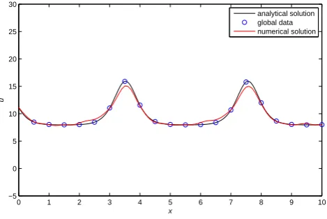
In the next experiments, Fig. 7, the perturbed analytical solution on the coarse grid was used for formation of the boundary conditions.

One can see that for the Cauchy-Dirichlet problem the nu-merical solution rather quickly diverges from the analytical solution due to the errors of the linear interpolation proce-dure in the border points. After 96 h, the perturbed boundary solution has very faint resemblance with the analytical one.

(8)

1.8 1.9 2 2.1 2.2 2.3 2.4 x 107 −4

−3 −2 −1 0 1 2 3 4 5

x 109

x (m)

ψ

(m

2/s)

analytical solution global data numerical solution

1.8 1.9 2 2.1 2.2 2.3 2.4

x 107 −4

−3 −2 −1 0 1 2 3 4 5

x 109

x (m)

ψ

(m

2/s)

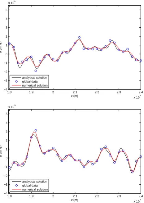
Fig. 8. Numerical solution of Rossby-Oboukhov equation by op-timization problem (red line) using 30% perturbed global model values (circles) att=48 h (upper panel), and at 96 h (lower panel).

1x=100 km,1t=3600 s. CPU time=0.5 s. Black line corresponds

to the reference analytical solution.

In the optimization approach one can use larger steps than in the Cauchy-Dirichlet problem, because we do not deal with a time-evolution problem, and there is no accumulation of numerical errors at each time step. In Fig. 8, one can see that, for space and time steps many times larger than those that were used in the Cauchy-Dirichlet problem (1x=10 km and1t=200 s), we have far better agreement with the ana-lytical solution. The decrease of time and/or space step in the optimization approach does not appreciably improve the solution. Only the smallest details are slightly better repro-duced.

Since the local mesh in the optimization approach is rather coarse, the average CPU time needed for solving the problem is smaller than for Cauchy-Dirichlet problem (0.5 s) in spite of greater computational complexity. Also we have to pay attention on a very weak sensitivity to the global data pertur-bations. The impact of earch individual perturbation on the optimization solution is very small. For example, increasing errors in randomly perturbed global data up to 60% does not strongly affect the solution as one can see in Fig. 9.

1.8 1.9 2 2.1 2.2 2.3 2.4

x 107

−4 −3 −2 −1 0 1 2 3 4 5

x 109

x (m)

ψ

(m

2/s)

Fig. 9. Numerical solution of Rossby-Oboukhov equation by opti-mization problem (red line) with 60% perturbed global model

val-ues (circles) att=96 h. 1x=100 km,1t=3600 s. CPU time=0.5 s.

Black line corresponds to the reference analytical solution.

With the above experiments we had the intention to show that even small errors in boundary conditions of the regional model can violently distort ideal solution (i.e., the one that is obtained when there are no errors in boundary condi-tions) However, applying optimization methods, and using the global data (from observation or from “global” model) available inside the regional domain (even containing the same kind of errors as the boundary conditions), gives us a way to avoid strong sensitivity of solution to boundary errors, allowing thus to obtain good results.

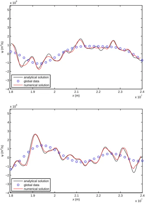
In our experiments the regional model has not the abil-ity to add small scale spectrum to the global model solution, because we use the same evolution model operator for both models. So, to simulate more realistic behavior let us modify the testing regional model.

First we generate more realistic global data omiting small scales. Using as the initial condition only the first 25 modes (the whole solution includes 85 modes) taken from analitical solution, showed on Fig. 5, we run the model with space and time steps equal to 100 km and 1800 s, respectively, on the entire periodic domain of 96 h. After that we extract from the obtained solution the global data, on the mesh with size 200 km and 2 h.

(9)

1.8 1.9 2 2.1 2.2 2.3 2.4 x 107

−4 −3 −2 −1 0 1 2 3 4 5

x 109

x (m)

ψ

(m

2/s)

1.8 1.9 2 2.1 2.2 2.3 2.4

x 107 −4

−3 −2 −1 0 1 2 3 4 5

x 109

x (m)

ψ

(m

2/s)

Fig. 10. Numerical Cauchy-Dirichlet problem solution of Rossby-Oboukhov equation (red line) with small scales introduced in the left side of boundary conditions (circles) att=48 h (upper panel)

and 96 h (lower panel). 1x=10 km, 1t=200 s. CPU time=0.8 s.

Black line corresponds to the reference analytical solution.

boundary due to interpolation. Using new regional model and global data without small scales we performed other ex-periments using traditional and optimization approaches, the results of which are showed in Figs. 10 and 11, respectively. These experiments clearly show that the use of additional global data inside the local domain, even perturbed ones, can significantly improve the solution of the model.

3.3 Korteweg-de Vries equation

The Korteweg-de Vries (KdV) equation is a nonlinear, dis-persive partial differential equation and represents a mathe-matical model of waves on shallow water surfaces:

ut+6uux+uxxx=0. (12)

1.8 1.9 2 2.1 2.2 2.3 2.4

x 107 −4

−3 −2 −1 0 1 2 3 4 5

x 109

x (m)

ψ

(m

2/s)

1.8 1.9 2 2.1 2.2 2.3 2.4

x 107 −4

−3 −2 −1 0 1 2 3 4 5

x 109

x (m)

ψ

(m

2/s)

Fig. 11. Numerical solution of Rossby-Oboukhov equation by

optimization problem (red line), using as global data (circles) the global model solution with 25 modes and additional small scales in the left boundary, att=48 h (upper painel) and at 96 h (lower painel).

1x=80 km,1t=2600 s. CPU time=1.25 s. Black line corresponds

to the reference analytical solution.

Equation (12) has the exact solution (Korteweg and de Vries, 1895; Grimshaw, 2004)

u(x, t )=b+acn2(γ (x−V t )|m), (13) where cn(x|m) is the Jacobi elliptic function, m∈(0,1) is the module of elliptic function, a=2mγ2 and V=6b+4(2m−1)γ2. For the case when m→1 we will have cn(x|m)→sech(x)and the solution (13) will have the form

(10)

−5 0 5 10 15 −5

0 5 10 15 20 25 30

x

u

Fig. 12. Analytical solution of KdV equation as the cnoidal wave

(13) on the domain [−5, 15] att=0 withγ=2, b=a and module

m=0.995.

For finite-difference discretization we use the following implicit numerical scheme (Furihata, 1999), which possesses the properties of total energy and mass conservation:

uj_i+1−uj_i 1t +

1 21x

(u_ij₊+₁1)2−(uj_i₋+₁1)2+u_ij₊+₁1uj_i₊₁−

uj_i₋+₁1uj_i₋₁+(u_ij₊₁)2−(uj_i₋₁)2+

1 21x3

uj_i₊+₂1+uj_i₊₂

2 −(u

j+1

i+1+u

j i+1)+

(uj_i₋+₁1+uj_i₋₁)−u j+1

i−2+u

j i−2 2

!

=0.

Since the numerical scheme is non-linear for numerical evaluation of Cauchy-Dirichlet problem we use Newton’s method for computinguj+1at each time step.

Following the steps of previous example, we choose as a reference model the analytical solution with cofficientsb=a, γ=2 and module of elliptic functionm=0.995. Figure 12 rep-resents the solution on the domain [−5, 15] at timet=0.

As a local model we consider the Eq. (12) defined over the closed interval [0, 10]. In order to get a good accordance be-tween a numerical solution of the Cauchy-Dirichlet problem (with exact initial and boundary conditions) and the analyti-cal solution on the time interval 0≤t≤1, showed in Fig. 13, we take as the maximum possible values of space and the time steps1x=0.02 and1t=0.0002, respectively. The CPU time required to find the solution is 15 s.

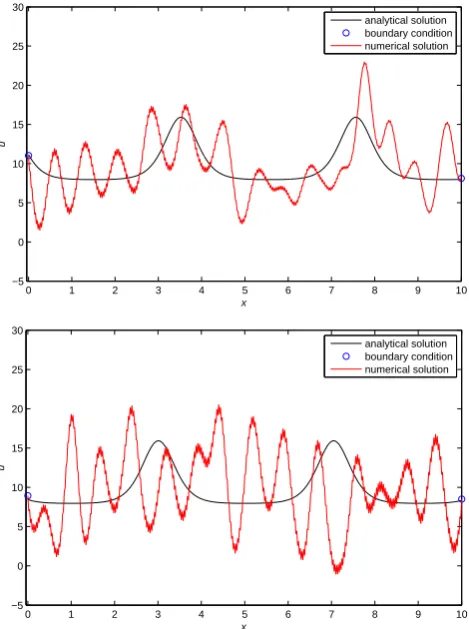
As a global model solution we take the analytical solu-tion, introduced above as the reference model, with space step1x=0.5 and time step1t=0.005 and perturb its values up to 10% from the exact ones. Using these perturbed global model solution to form the boundary condition we solve the Cauchy-Dirichlet problem.

In Fig. 14 one can see that the Cauchy-Dirichlet problem with small errors in the boundary conditions can produce un-acceptable numerical solutions.

0 1 2 3 4 5 6 7 8 9 10

−5 0 5 10 15 20 25 30

x

u

Fig. 13. Numerical Cauchy-Dirichlet problem solution of KdV equation with exact boundary condition (red line) att=1.1x=0.02,

1t=0.0002. CPU time=15 s. Black line corresponds to the

refer-ence analytical solution.

0 1 2 3 4 5 6 7 8 9 10

−5 0 5 10 15 20 25 30

x

u

0 1 2 3 4 5 6 7 8 9 10

−5 0 5 10 15 20 25 30

x

u

Fig. 14. Numerical Cauchy-Dirichlet problem solution of KdV equation (red line) with 10% perturbed boundary condition (circles)

at timet=0.5 (upper panel), and t=1.0 (lower panel). 1x=0.02,

1t=0.0002. CPU time=23 s. Black line corresponds to the

(11)

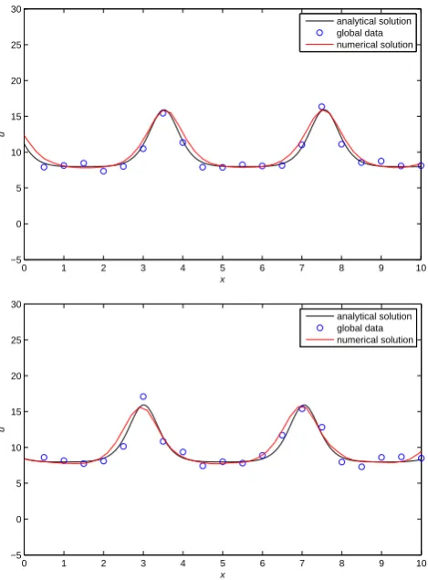
Now, we apply the optimization method to the local model using all the avaliable points of the global model solution. Figure 15 shows the solution of the optimization problem. As in the previous experiment we choose the space (1x=0.2) and the time (1t=0.002) steps as large as possible.

It can be clearly seen the advantage of the optimization approach in this case. The difference between numerical and exact solution is very small in comparison with the Cauchy-Dirichlet problem calculations.

4 Conclusions and discussions

The results of the numerical experiments presented here in-dicate that the optimization approach can significantly im-prove the precision of the numerical solution of the regional model when the boundary values have errors but informa-tion in a number of inner points is available. Even in the cases in which the solution of the Cauchy-Dirichlet problem is very sensitive to the errors in the boundary condition, the use of optimization approach gives the possibility to compute solutions that are close to the analytical solution. We also made experiments with two-dimensonal nonlinear Rossby-Oboukhov equations. The preliminary results demonstrate as well that the use of the optimization approach significantly improve the numerical solution.

Applying 4D-Var data assimilation to limited-area prob-lem has some common features with the optimization ap-proach used here. In a series of works devoted to optimal control of initial and lateral boundary conditions it is empha-sized the strong sensitivity of obtained solution to the lateral baundary data (Griffin and Thomson, 1996; Lu and Brown-ing, 2000; Zou and Kuo, 1996; Leredde et al., 1998). As it was shown in the above mentioned papers, the consistency of lateral boundary conditions with another “observation” data permit to obtain more realistic regional model fields. In our approach this consistency between “regional model” and “global model” is assured automatically by optimization so-lution procedure for the whole soso-lution period.

In connection with applying a deterministic 4D-Var scheme to find the most likely model evolution fitting ob-servations, (Lorenc and Payne, 2007) pointed out that it does not work in the limit of high resolution. On the other hand, Statistical 4D-Var (Lorenc, 2003) is a suitable alternative. The reason is that deterministic 4D-Var aims to find the most probable solution, which corresponds to the mode of the probability distribution function whereas statistical 4D-Var seeks an efficient approximation to the probability density function expectation. Let us interpret the observations of Lorenc and Payne in optimization terms and see how they apply to our case. For simplicity, the independent variables are denoted byxso that our problem is to minimizef (x)(the error) subject tox∈(the model). The mode solution corre-sponds to the global minimizer off. The choice of the global minimizer as the best solution may be challenged if the basin

0 1 2 3 4 5 6 7 8 9 10

−5 0 5 10 15 20 25 30

x

u

0 1 2 3 4 5 6 7 8 9 10

−5 0 5 10 15 20 25 30

x

u

Fig. 15. Numerical solution of KdV equation by optimization prob-lem (red line) with 10% perturbed global data (circles) at timet=0.5 (upper panel), and att=1.0 (lower panel).1x=0.2,1t=0.002. CPU time=21 s. Black line corresponds to the reference analytical solu-tion.

(12)

0 1 2 3 4 5 6 7 8 9 10 −5

0 5 10 15 20 25 30

x

u

Fig. A1. Numerical evolutionary (Cauchy-Dirichlet problem) so-lution of KdV equation using center-space and center-time scheme (red line) after 40 steps with1x=0.1 and1t=5∗10−4. Black line corresponds to the reference analytical solution.

Appendix A

Formulation of optimization problem

We can express our problem as the following non-linear op-timization problem with equality constraints

Minimize 1₂ku−Vk2 P

s.t. h(u)=0, (A1)

where V represents the global data on the re-gional mesh, P is the diagonal penality matrix and h(u)=[h1(u) h2(u) . . . hm(u)]T is a vector of the

discretiza-tions of regional equadiscretiza-tions at each point of space-time mesh of the regional model.

A usual optimization technique to solve this kind of prob-lem is to apply Newton’s iteration method to the system of nonlinear equations arising from first-order necessary con-ditions, known as Karush-Kuhn-Tucker (KKT) conditions (Nocedal and Wright, 1999). For instance, the KKT con-ditions for the problem (A1) are

P (u−V )+h0(u)Tλ=0

h(u)=0, (A2)

where

h0(u)=



     

∇h1(u)T

∇h2(u)T .. .

∇hm(u)T



     

is the Jacobian matrix of the constraint function and λ represent the vector of Lagrange multipliers. Each step of the Newton iteration associated with system (A2) is defined

as follows:

J (uk, λk)

1uk

1λk

=−

P (uk−V )+h0(uk)Tλk

h(uk)

uk+1 λk+1

=

uk

λk

+

1uk

1λk

(A3)

whereJ represents the Jacobian matrix of the system (A2)

J (u, λ)=



 P+P

iλi∇2hi(u) h0(u)T

h0(u) 0 

, (A4)

and∇2hi(u),i=1, . . . , m, are Hessian matrices of the

con-straints.

The Jacobian matrix (A4) is a saddle point matrix and there are many methods that can be applied for the associated linear system (Benzi, Golub and Liesen, 2005). However, note that the Jacobian of the constraintsh0(u)is described by a sparse matrix with block-diagonal structure. On the other hand, the first partP+P

iλi∇2hi(u)of the Jacobian matrix

(A4) of the system (A2) includes the calculation of the Hes-sians of the constraints, which is computationally expensive because calculations have to be made for every Newton iter-ation. The resulting matrix is generally dense. To accelerate the calculations and reduce the computer memory require-ments we use the following Jacobian approximation:

Bk=

P h0(uk)T

h0(uk) 0

. (A5)

The use of the approximation Bk for J (uk, λk)strongly

simplifies the procedure of finding the solution of the linear system (A3).

Appendix B

Mesh size on optimization approach

To describe the same space and time scales, the optimiza-tion approach can use larger space and time steps than the traditional evolutionary approach. The key to explain this phenomenon is that the optimization algorithm is non-evolutionary in time, hence it is not necessary to satisfy the stability condition. Moreover, there is no accumulation of discretization error. Therefore, for any period of integration, space and time steps depend only on the scales of the process of interest.

(13)

0 1 2 3 4 5 6 7 8 9 10 −5

0 5 10 15 20 25 30

x

u

Fig. B1. Numerical evolutionary (Cauchy-Dirichlet problem) so-lution of KdV equation using center-space and center-time scheme (red line) at timet=0.5 with1x=0.1 and1t=4.5∗10−4. Black line corresponds to the reference analytical solution.

0 1 2 3 4 5 6 7 8 9 10

−5 0 5 10 15 20 25 30

x

u

Fig. B2. Numerical evolutionary (Cauchy-Dirichlet problem) so-lution of KdV equation using center-space and center-time scheme (red line) at timet=0.5 with1x=0.04 and1t=2∗10−5. Black line corresponds to the reference analytical solution.

center-time scheme for discretization of the KdV equation uk_i+1−uk_i−1

21t +6u

k i

uk_i₊₁−uk_i₋₁

21x +

uk_i₊₂−2uk_i₊₁+2uk_i₋₁−uk_i₋₂

21x3 =0

and taking the space step1x=0.1, we obtain the stable solu-tion, by traditional approach, only for time steps1t≤4.5∗

10−4. Figure A1 shows the instability of scheme for time step1t=5∗10−4after 40 steps.

0 1 2 3 4 5 6 7 8 9 10

−5 0 5 10 15 20 25 30

x

u

Fig. B3. Numerical optimization solution of KdV equation using center-space and center-time scheme (red line) at timet=0.5 with

1x=0.04 and1t=2.5∗10−3. Black line corresponds to the refer-ence analytical solution, circles marks global data.

0 1 2 3 4 5 6 7 8 9 10

−5 0 5 10 15 20 25 30

x

u

Fig. B4. Numerical optimization solution of KdV equation using center-space and center-time scheme (red line) at timet=0.5 with

1x=0.1 and1t=2.5∗10−3. Black line corresponds to the reference analytical solution, circles marks global data.

In addition to this, for long time evolutions the accumula-tion of discretizaaccumula-tion error tends to be more significant. As we can see in Fig. B1, for time period 0.5 space step1x=0.1 and time step1t≤4.5∗10−4_{produce a bad result. So it is} necessary to refine the mesh when the period of integration becomes longer. In the case of t=0.5 a resonable result is achieved for1x=0.04 and1t=2∗10−5(see Fig. B2).

(14)

As we can see, for the optimization approach there is no the same concept of stability as for the forward problem. Be-sides allowing a larger time step, the optimization approach also allows the use of a larger space step, since there is no accumulation of discretization error, as we mentioned above. Figure B4 shows the optimization solution for1x=0.1 and 1t=2.5∗10−3

Acknowledgements. The authors gratefully acknowledge

R. Laprise for constructive discussions which helped to make clear a number of difficulties of the problem, and T. A. Tarasova for useful comments on the text that significantly improved the

manuscript. The authors also express great gratitude to editor

O. Talagrand and two referees for valuable remarks and useful references.

F. I. Pisnitchenko was supported by FAPESP (Grant 03-09938-0); J. M. Mart´ınez was supported by FAPESP (Grant 06-53768-0) and CNPq and S. A. Santos was supported by CNPq.

Edited by: O. Talagrand

Reviewed by: A. Lorenc and another anonymous referee

References

Andreani, R., Birgin, E. G., Mart´ınez, J. M., and Schuverdt, M. L.: On Augmented Lagrangian methods with general lower-level constraints, SIAM J. Optimiz., 18, 1286–1309, 2007.

Andreani, R., Birgin, E. G., Mart´ınez, J. M., and Schuverdt, M. L.: Augmented Lagrangian methods under the Constant Posi-tive Linear Dependence constraint qualification, Math. Program., 111, 5–32, 2008.

Benzi, M., Golub, G. H., and Liesen, J.: Numerical Solution of Saddle Point Problems, Acta Numerica, 1–137, Cambridge Uni-versity Press, 2005.

Birgin, E. G. and Evtushenko, Y.: Automatic differentiation and spectral projected gradient methods for optimal control prob-lems, Optimization methods and software, 10, 20–42, 1998. Birgin, E. G. and Mart´ınez, J. M.: Improving ultimate convergence

of an Augmented Lagrangian method, Optimization Methods and Software, 23, 177–195, 2008.

Boh´e, A.: The existence of supersensitive boundary-value prob-lems, Methods and Applications of Analysis, 3(3), 318–334, 1996.

Denis, B., Laprise, R., and Caya, D.: Sensitivity of a regional cli-mate model to the resolution of the lateral boundary conditions, Clim. Dynam., 20, 107–126, 2003.

Diaconescu, E. P., Laprise, R., and Sushama, L.: The impact of lateral boundary data errors on the simulated climate of a nested regional climate model, Clim. Dynam., 28, 333–350, 2007. Errico, R. M.: What is an adjoint model?, B. Am. Metor. Soc., 78,

2577–2591, 1997.

Ferreira-Mendonca, L., Lopes, V. L. R., and Marinez, J. M.: Quasi-Newton Acceleration for Equality Constrained Minimization, Comput. Optim. Appl., 40, 373–388, 2008.

Fisher, M., Nocedal, J., Tremolet, Y., and Wright, S. J.: Data Assimilation in Weather Forecasting: A Case Study in

PDE-Constrained Optimization, Technical Report, Optimization Tech-nology Center, 2006.

Furihata, D.: Finite difference schemes for ∂u_∂t=

∂ ∂x

α

δG δu that

inherit energy conservation or dissipation property, J. Comput. Phys., 156, 181–205, 1999.

Gershunov, A., Barnett, T. P., Cayan, D. R., Tubbs, T., and Goddard, L.: Predicting and Downscaling ENSO Impacts on Intraseasonal Precipitation Statistics in California: The 1997/1998 Event, J. Hydrometeorol., 1, 201–210, 2000.

Griffin, D. A. and Thomson, K. R.: The adjoint method for data assimilation used operationally for shelf circulation, J. Geophys. Res., 101(C2), 3457–3477, 1996.

Griewank, A.: On Automatic Differentiation, Mathematical Pro-gramming: Recent Developments and Applications, Kluwer Academic Publishers, 83–108, 1989.

Grimshaw, R.: Korteweg-de Vries equation. Encyclopedia of Non-linear Science, edited by: Scott, A. C., Taylor and Francis, New York, 504–511, 2004.

Kanamaru, H. and Kanamitsu, M.: Scale selective bias correction in a downscaling of global analysis using a regional model, Cal-ifornia energy commission, PIER energy-related environmental research, CEC-500-2005-130, 2005

Korteweg, D. J and de Vries, H.: On the Change of Form of Long Waves advancing in a Rectangular Canal and on a New Type of Long Stationary Waves, Philosophical Magazine, 5th series, 36, 422–443, 1895.

Le Dimet, F.-X. and Talagrand, O.: Variational algorithms for anal-ysis and assimilation of meteorological observations: theoretical aspects, Tellus, 38A, 97–110, 1986.

Leredde, Y., Lellouche, J.-M., Devenon, J.-L., and Dekeyser, I.: On initial, boundary and viscosity coefficient control for Burgers’ equation, Int. J. Numer. Meth. Fluids, 28, 113–128, 1998. Lorenc, A. C.: Modelling of error covariances by 4D-Var data

as-similation, Q. J. Roy. Meteor. Soc., 129, 3167–3182, 2003. Lorenc, A. C. and Payne, T.: 4D-Var and the butterfly effect:

Sta-tistical four-dimensional data assimilation for a wide range of scales, Q. J. Roy. Meteor. Soc., 133, 607–614, 2007.

Lu, C. and Browning, G. L.: Four-dimensional variational data as-similation for limited-area models: lateral boundary conditions , solution uniqueness, and numerical convergence, J. Atmos. Sci., 57, 1341–1353, 2000.

Mart´ınez, J. M.: Practical quasi-Newton methods for solving non-linear systems, J. Comput. Appl. Math., 124, 97–122, 2000. Nocedal, J. and Wright, S. J.: Numerical Optimization, Springer

Verlag, 1999.

Obukhov(Oboukhov), A. M.: On the question of the geostrophic wind, Izv. Akad. Nauk SSSR Ser. Geograf-Geofiz., 13, 281–306, 1949.

Rabier, F.: Overview of global data assimilation developments in Numerical Weather Prediction centres, Q. J. Roy. Meteor. Soc., 131, 3215–3233, 2005.

Rossby, C.-G.: Relation between variations in the intensity of the zonal circulation of the atmosphere and the displacements of the semi-permanent centers of action, J. Marine Res., 2, 38–55, 1939.

(15)

von Storch, H., Langenberg, H., and Feser, F.: A spectral nudging technique for dynamical downscaling purposes, Mon. Weather Rev., 128, 3664–3673, 2000.

Waldron, K. M., Peagle, J., and Horel, J. D.: Sensitivity of a spec-trally filtered and nudged limited-area model to outer model op-tions, Mon. Weather Rev., 124, 529–547, 1996.