A Comparison of Some Bayesian and Classical Procedures for Simultaneous Equation Models with Weak Instruments

(1)

Article

A Comparison of Some Bayesian and Classical

Procedures for Simultaneous Equation Models with

Weak Instruments

Chuanming Gao1_{and Kajal Lahiri}2,_*

1 _{Fannie Mae, 1100 15th St NW, Washington, DC 20005, USA}

2 _{Department of Economics, University at Albany, SUNY, Albany, NY 12222, USA}

* Correspondence: [email protected]

Received: 18 March 2019; Accepted: 23 July 2019; Published: 29 July 2019

Abstract:We compare the finite sample performance of a number of Bayesian and classical procedures for limited information simultaneous equations models with weak instruments by a Monte Carlo study. We consider Bayesian approaches developed by Chao and Phillips, Geweke, Kleibergen and van Dijk, and Zellner. Amongst the sampling theory methods, OLS, 2SLS, LIML, Fuller’s modified LIML, and the jackknife instrumental variable estimator (JIVE) due to Angrist et al. and Blomquist and Dahlberg are also considered. Since the posterior densities and their conditionals in Chao and Phillips and Kleibergen and van Dijk are nonstandard, we use a novel “Gibbs within Metropolis–Hastings” algorithm, which only requires the availability of the conditional densities from the candidate generating density. Our results show that with very weak instruments, there is no single estimator that is superior to others in all cases. When endogeneity is weak, Zellner’s MELO does the best. When the endogeneity is not weak andρω12 >0, whereρis the correlation coefficient between the structural and reduced form errors, andω12is the covariance between the unrestricted reduced form errors, the Bayesian method of moments (BMOM) outperforms all other estimators by a wide margin. When the endogeneity is not weak andβρ<0 (βbeing the structural parameter), the Kleibergen and van Dijk approach seems to work very well. Surprisingly, the performance of JIVE was disappointing in all our experiments.

Keywords: limited information estimation; weak instruments; Metropolis–Hastings algorithm; Gibbs sampler; Monte Carlo method

JEL Classification:C30; C11; C13; C15

1. Introduction

Research on Bayesian analysis of the simultaneous equations models addresses a problem, raised initially byMaddala(1976), and now recognized as related to the problem of local nonidentification when diffuse/flat priors are used in traditional Bayesian analysis, e.g.,Drèze(1976);Drèze and Morales (1976), and Drèze and Richard (1983).1 In this paper, we examine the approaches developed by Chao and Phillips (1998, hereafter CP), Geweke (1996), Kleibergen and van Dijk(1998, hereafter KVD), andZellner(1998). The idea in KVD was to treat an overidentified simultaneous equations

1 _Zellner₍₁₉₉₈_{) and}_{Zellner et al.}₍₂₀₁₄_{) contain a comprehensive review of the finite sample properties of SEM estimators,} and emphasize the need for finite sample optimal estimation procedure for such models.Andrews and Stock(2005) reviews recent developments in methods that deal with weak in IV regression models, and presents new testing results under “many weak-IV asymptotics”.

(2)

model (SEM) as a linear model with nonlinear parameter restrictions, and has been extended further in Kleibergen and Zivot (2003). While KVD focused mainly on resolving the problem of local nonidentification, CP explored further the consequences of using a Jeffreys prior. By deriving the exact and (asymptotically) approximate representations for the posterior density of the structural parameter, CP showed that the use of a Jeffreys prior brings Bayesian inference closer to classical inference in the sense that this prior choice leads to posterior distributions which exhibit Cauchy-like tail behavior akin to the LIML estimator. Geweke(1996), being aware of the potential problem of local nonidentification, suggests a shrinkage prior such that the posterior density is properly defined for each parameter. In another approach,Zellner(1998) suggested a finite sample Bayesian method of moments (BMOM) procedure based on given data without specifying a likelihood function or introducing any sampling assumptions.

For the Bayesian approaches considered, whileGeweke(1996) proposed Gibbs sampling (GS) to evaluate the posterior density with a shrinkage prior, the posterior densities as well as their conditional densities resulting from CP and KVD are nonstandard and cannot be readily simulated. In the category of “block-at-a-time” approach, we suggest a novel MCMC procedure, which we call a “Gibbs within M–H” algorithm. The advantage of this algorithm is that it only requires the availability of the conditional densities from the candidate generating density. These conditional densities are used in a Gibbs sampler to simulate the candidate generating density, whose drawings on convergence are then weighted to generate drawings from the target density in a Metropolis–Hastings (M–H) algorithm. In this study, we will focus on weak instruments, where the classical approach has been particularly problematic.2 _{Ni and Sun}_{(2003) have studied similar issues in the context of vector autoregressive} models, see alsoNi et al.(2007).Radchenko and Tsurumi(2006) used many of the procedures analyzed in this paper to estimate a gasoline demand model using an MCMC algorithm.

The main objective of the present paper is to compare the small sample performance of some Bayesian and classical approaches using Monte Carlo simulations. For the purpose of comparison, a number of classical methods including OLS, 2SLS, LIML, Fuller’s modified LIML, and a jackknife instrumental variables estimator (JIVE) originally due toAngrist et al. (1999) and Blomquist and Dahlberg(1999) are also computed from the generated data. Our simulation results from repeated sampling experiments provide some unambiguous guidelines for empirical practitioners.

The plan of the paper is as follows. In Section2, we set up the model. Section 3reviews in limited details the recent Bayesian approaches and JIVE. Section4suggests a new MCMC procedure for evaluating the posterior distributions for CP and KVD, and discusses the convergence diagnostics implemented. Section5presents simulation results and some discussions. Section6contains the main conclusions.

2. The Model

Consider the following limited information formulation of the m-equation simultaneous equations model (LISEM):

y1=Y2β+Z1γ+u (1)

Y2=Z1Π1+Z2Π2+V2 (2)

wherey1: (T ×1) andY2: (T×(m−1)) are the m included endogenous variables; Z1: (T×k1) is an observation matrix of exogenous variables included in the structural Equation (1);Z2:(T×k2) is an observation matrix of exogenous variables excluded from (1); anduandV2are, respectively, aT×₁

vector and aT×₍_m−_{1) matrix of random disturbances to the system. We assume that (}_u_,_V2₎∼_N

2 _{There has been a lot of interest in the estimation of LISEM with weak instruments. See}_Buse₍₁₉₉₂_);_{Bound et al.}₍₁₉₉₅_);

(3)

(0,Σ⊗_I_T₎_,_{where the}_m×_m_{covariance matrix is positive definite symmetric (pds) and is partitioned}

conformably with the rows of (u,V2) as follows

Σ= σ11 σ

0

21 σ₂₁ Σ₂₂

!

The likelihood function for the model described by (1) and (2) can be written as

L(β,γ,Π1,Π2,Σ|Y,Z) = (2π)−Tm/2|Σ|−T/2_expn−1

2tr h

Σ−₁

(u,V2)

0

(u,V2) io

, (3)

whereY= (y1,Y2)andZ= (Z1,Z2).

The structural model described by (1) and (2) can alternatively be written in its reduced form

y1 Y2

= Z1 Z2

π₁ Π₁

Π2β Π2 !

+ ξ₁ V2 (4)

where π1 = γ+Π1β,ξ1 = u+V2β, (ξ1, V2) ∼ N(0,Ω⊗IT), andΣ = C0ΩC, C = ₋1_β 0

Im−₁

! .

The likelihood function corresponding to this alternative representation is:

L(β,γ,Π1,Π2,Ω|Y,Z) = (2π)

−_Tm_/2

|Ω|−T/2_exp{−1

2tr h

Ω−₁

(ξ1,V2)

0

(ξ1,V2) i

} ₍₅₎

The likelihood functions (3) and (5) are equivalent since the Jacobian betweenΩandΣis unity. Geweke(1996) considers the following reduced rank regression specification3

Y=Z1A+Z2Θ+E, (6)

where A= (Π₁,π1),Θ=Π2ΦandΦ= (Im−₁, β), E= (V2,ξ₁)~N(0,Σ⊗ITwithΣ−1= Σ

11 _Σ12

Σ21 _Σ22 !

partitioned conformably with the rows of (V2,ξ1). Obviously, (6) is equivalent to (4) and the corresponding likelihood function is similar to (5).

Note that in the absence of restrictions on the covariance structure, (1) is fully identified if and only ifrank(Π₁) = (m−₁)≤_k2_.

3. Review of Some Bayesian Formulations

Among the Bayesian approaches,Geweke(1996) used a shrinkage prior such that all parameters are identified (in the sense that a proper posterior distribution exists) even whenΠ2has reduced rank. KVD treated overidentified SEMs as linear models with nonlinear parameter restrictions using the singular value decomposition. A diffuse or natural conjugate prior for the parameters of the embedding linear model results in the posterior for the parameters of the SEM having zero weight in the region of parameter space whereΠ2has reduced rank. This is a feature of the Jacobian of transformation from the multivariate linear model to the SEM. CP used a prior by applying Jeffreys principle on the model described by (1) and (2) and the assumptions regarding the disturbances. An important advantage of the Jeffreys prior in the present context is that it places no weight in the region of the parameter space whererank(Π2)<(m−1)and relatively low weight in close neighborhoods of this region where the model is nearly unidentified.

(4)

3.1. Zellner’s Bayesian Method of Moments Approach (BMOM)

Among the various Bayesian treatments of SEM proposed byZellner(1971,1978,1986,1994,1998), the Bayesian method of moments approach applies the principle of maximum entropy and generates optimal estimates which can be evaluated by double K-class estimators. Given the unrestricted reduced form equationy1=Zπ1+ξ1,Zellner(1998) considered a balanced loss function,

Lb =ωLg+ (1−ω)Lp

=ωy1−_Xδˆ 0

y1−_Xδˆ+ (1−ω)Zπ1−Xδˆ 0

Zπ1−Xδˆ

, for 0≤ω≤₁

whereX= (Y2,Z1),δ= (β0,γ0), and ˆδis an estimate ofδ. The BMOM estimate that minimizesELb,

where the expectation is taken with respect to a probability density function of theπmatrices of the unrestricted reduced form equations, is given by

ˆ

β

ˆ

γ

!

= Y

0

2Y2−K1Vˆ

0

2V2ˆ Y

0

2Z1 Z0₁Y2 Z0₁Z1

!−1     

Y2−K2Vˆ2 0

y1 Z0₁y1

    

, (7)

whereK1=1 − _k_/_(T−_k)_, _K2₌ ₁− ₍₁−ω_)k_/_(T−_k)_{with 0} ≤ω≤_{1 and ˆ}_V2₌_I−_Z(Z0_Z)−1_Z0_Y2_.

BMOM estimate will vary depending on the value ofω. Whenω=1, it is the optimal estimate resulting from a “goodness of fit” loss functionLg. Whenω=0, it is the optimal estimate given by a precision of estimation loss functionLp. Meanwhile, the well-known minimum expected loss (MELO)

estimator is derived using a precision of estimation loss function and may be evaluated as a K-class estimator with

K1=K2=1−_k_/_(T−_k−_m−₁₎_.

Similar to the BMOM method,Conley et al.(2008) developed a Bayesian semiparametric approach to the instrumental variable problem assuming linear structural and reduced form equations, but with unspecified error distributions.

3.2. The Geweke Approach

Geweke(1996) assumes the following reference prior

Σ

−₍_m₊_v_+1)/2

exp

−1

2trSΣ

−₁

exp "

−τ 2

2

β0

β+trΠ0₂Π2+trA

0

A #

, (8)

which is the product of an independent inverted Wishart distribution forΣwithvdegrees of freedom and scale matrix S, and an independentN(0,τ2) shrinkage priors for each element ofβandΠ2. Geweke derived the respective conditional posterior distributions, which may be used to generate drawings through Gibbs sampling from the joint posterior distribution. Regarding the vector of parameters

Σ−₁

, A,Π2,β

, we obtain the full conditional densities as follows:

(1) Conditional density ofΣ−1

Σ−₁

(Π2,β, A,Z,Y) ∼Wishart

T+v, G−1, (9)

(5)

(2) Conditional density of A

vec(A)

Π2,β,Σ−1, Z, Y

∼_N(hΣ−1⊗_Z0

1Z1+τ2Imk1 i−1h

Σ−₁_⊗

Z1

0

Z1 i

vec(Aˆ), h

Σ−₁ ⊗_Z0

1Z1 +τ 2_I

mk₁

i−1 ),

(10)

where ˆA =Z0₁Z1

−₁

Z0₁(Y − _Z2Θ). (3) Conditional density ofΠ24

vec(Π2)

β,Σ−1, A, Z, Y

∼_N(

e

Σ11⊗_Z0

2Z2+τ2Ik2(m−1) −1

e

Σ11⊗_Z0

2Z2

vec(Πˆ₂),

e

Σ11⊗_Z0

2Z2+τ2Ik2(m−1) −1

),

(11)

where ˆΠ2=Θˆ "

Φ+₊_Φ0 eΣ

21 e

Σ11

−₁#

, ˆΘ = Z0₂Z2−1Z0₂(Y−_Z₁_A₎_. Φ+ _{is the Moore–Penrose}

generalized inverse of Φand the columns ofΦ+ and Φ0are orthogonal, and C≡ ₍Φ+_, Φ0₎

is and m ×_{m nonsingular matrix. Finally,} eΣ

i j

denotes the partitioning ofeΣ

−₁

= (C0ΣC)−1 conformably withY= (Y2,y1).

(4) Conditional density ofβ

β

Π2,Σ−1, A,Z, Y

∼ _N

_h

Σ22_⊗_Π0

2Z

0

2Z2Π2+τ2Im−₁

i−1h

Σ22_⊗_Π0

2Z

0

2Z2Π2 i

ˆ

β,hΣ22⊗Π0 2Z

0

2Z2Π2+τ2Im−₁

i−1 , (12)

where

ˆ

β=Π0₂Z0₂Z2Π2 −1

Π0

2Z

0

2(Y2−Z1Π1)Σ 12

Σ22−1

− Σ12Σ22 −₁

+Π0₂Z0₂Z2Π2 −1

Π0

2Z

0

2(y1−Z1π1)

3.3. The Chao and Phillips Approach

Using Jeffreys prior, CP obtains exact and approximate analytic expressions for the posterior density of the structural coefficientβin the LISEM (1) and (2). Their formulas are found to exhibit Cauchy-like tails analogous to comparable results in the classical literature on LIML estimation. For the model (1) and (2) under normality assumption for the disturbances, a Jeffreys prior on the parameters,

θ= (β,γ,Π1,Π2,Σ),is of the form

p(β,γ,Π1,Π2,Σ)∝ −_E ( ∂2

∂θ∂θ0lnL(θ|Y,Z)

) 1/2

∝ |_σ₁₁|(k2−m+1)/2|Σ|−(k+m+1)/2 Π

0

2Z

0

2QZ1Z2Π2

1/2

(13)

where ln L(θ

Y, Z) is the log-likelihood function as specified in (3), andQX = IT− PX, PX = X(X0X)−1X0. As first noted byPoirier(1996), the prior in (13) places no weight whererank(Π2)<(m−1) through the factor

Π

0

2Z

0

2QZ1Z2Π2

1/2 .

4 _{The expressions for the conditional densities of}_Π

(6)

The joint posterior of the parameters of LISEM (1) and (2) is constructed as proportional to the product of the prior (13) and the likelihood function (3),

p(β,γ,Π1,Π2,Σ

Y,Z)∝p(β,γ,Π1,Π2,Σ)L(β,γ,Π1,Π2,Σ|Y,Z)

∝ |_σ₁₁|(k2−m+1)/2|Σ|−(T+k+m+1)/2 Π

0

2Z

0

2QZ1Z2Π2

1/2

×_exp{−1

2tr h

Σ−₁

(u,V2)

0

(u,V2) i

} ₍₁₄₎

where (u,V2) is defined in (1) and (2). Note that (14) or its conditionals do not belong to any standard class of probability density functions.

3.4. The Kleibergen and van Dijk Approach

To solve the problem of local nonidentification and to avoid the so-called Borel–Kolmogorov paradox, seeBillingsley(1986) andPoirier(1995), KVD considered (4) as a multivariate linear model with nonlinear parameter restrictions:

y1 Y2 = Z1 Z2 π1 Π1 φ₂ Φ₂

!

+ ξ1 V2

, (15)

whereφ₁ is ak2×_{1 vector,}Φ₂ _{is a}_k2×_(m−₁₎_{matrix. Denote}Φ _{= (}_φ₁_,Φ₂₎_{. The reduced form}

model (4) is obtained if a reduced rank restriction is imposed on the linear model (15) such that rank(Φ) = (m−₁₎_{instead of}_m_.

Using a singular value decomposition (SVD) ofΦ, they show that (15) is identical to the so-called unrestricted reduced form (URF) model,5

y1 Y2

=Z1

π1 Π1

+Z2Π2B+Z2Π2⊥λB⊥+

ξ1 V2

, (16)

where B= β Im−₁

,λis a(k2−_m−₁)×_{1 vector.} Π₂⊥and B⊥are the orthogonal complements of

Π2and B, respectively, such thatΠ0₂Π2⊥≡0, BB 0

⊥≡0, andΠ 0

2⊥Π2⊥≡Ik2−m−1, B⊥B

0

⊥≡ 1 (i.e.,Π2⊥=

−Π₂₂Π−1 21 Ik2−m−1

0

Ik2−m−1+Π22Π

−₁

21Π

−₁0 21 Π22

−1/2

, whereΠ2=

Π0

21Π

0

22 0

,Π21 : (m−1)×(m−1),

Π22: (k2−m−1)×(m−1), and B⊥= (1+β0β)1/2(1−β0)).

There is one-to-one correspondence between the parameters in (15) and (16). The SVD ofΦis,

Φ = USV0, (17)

whereU: k2× k2,U0U=Ik2;V: m×m;V

0

V=Im; and S : k2× mis a rectangular matrix containing the (nonnegative) singular values (in decreasing order) on its main diagonal (i.e., (s11, s11,. . .,smm)). Rewrite

U= U11 U12 U21 U22

!

,= S1 0 0 S2

!

, and V= v11 v12 v21 v22

!

, (18)

whereU11, S1,v21 : (m−1)×(m−1);v12 : 1×1;v₁₁0 ,v22 : (m−1)×1;U12 : (m−1)×(k2−m+1)× (m−₁₎_;_U₂₁_:_(k₂−_m−₁₎×_(m−₁₎_;_U₂₂_: _(k₂ − _m−₁₎×_(k₂−_m₊₁₎_{; S}₂_: _(k₂ − _m−₁₎×_{1, then the}

following relationship between (Π2,β, λ) and(U, S, V) results,Π2= U11 U12

!

S1V0₂₁,β=V0−₂₁1v0₁₁, and

λ=U22U₂₂0

−_1/2

U22S2v0₁₂v12v0₁₂

−_1/2

. (19)

(7)

Note thatλis obtained through pre- and postmultiplication of s2by orthogonal matrices while s2 contains the smallest singular values ofΦand is invariant with respect to the ordering of variables contained inYandZ2.

According to KVD, the above shows that the model described by (1) and (2) can be considered as equivalent to the linear model (16) with a nonlinear (reduced rank) restrictionλ=0 on the parameters. Therefore, the priors and posteriors of the parameters of the LISEM (1) and (2) may be constructed as proportional to the priors and posteriors of the parameters of the linear model (16) evaluated atλ=0.

A diffuse (Jeffreys) prior for the parameters (π1,Π1,Φ,Ω) of the linear model6

p(π1,Π1,Φ,Ω)∝ |Ω|

−₍_k₊_m_+1)/2_{∝ |}

Ω|−(m+1)/2 Ω

−₁_⊗

Z0Z

1/2

(20)

wherek=k1+k2, implies the prior for the parameters (β,π1,Π1,Π2,Ω) of the LISEM (4) as

p(β, π1,Π1,Π2,Ω)∝p(π1,Π1Φ(Π2, β,λ),Ω)|λ=0|J(Φ,(Π2,β,λ)) λ=0

∝ |Ω|−(m+1)/2 Ω

−₁ ⊗_Z0_Z

1/2

J(Φ,(Π2,β,λ)) _λ₌₀

∝ |Ω|−(m+1)/2 Ω

−₁_⊗

Z0Z 1/2 ×

B0 ⊗ _I_k

2 e1 ⊗ Π2B

0

⊥⊗ Π2⊥

,

(21)

wheree1 = (1, 0, 0,. . ., 0)0. Note that the prior (21) is the Jeffreys prior of the unrestricted reduced form (16) evaluated atλ=0. Most importantly,|J(Φ, (Π2,β,λ))|λ=0=0 whenΠ2has reduced rank. This feature in KVD approach eliminates the potential impact of local nonidentification.

The joint posterior of the parameters of the LISEM (4) is readily constructed as proportional to the product of the prior (21) and the likelihood function (5),

p(β, π1,Π1,Π2,Ω Y, Z)

∝_p(β_,π₁_,Π₁_,Π₂_, Ω_)L∗

(β, γ,Π1,Π2,Ω

Y, Z)∝ |Ω|

−₍_T₊_m_+1)/2 Ω

−₁_⊗

Z0 Z 1/2 ×

B0⊗_I_k

2 e1⊗Π2B

0

⊥⊗Π2⊥

×_exp{−1 2tr[Ω

−₁

( y1 Y2 − _Z1 _Z2 π1 Π1

Π2β Π2 !

)

0

( y1 Y2

− _Z₁ _Z₂ π1 Π1

Π2β Π2 !

)]}

(22)

Unfortunately, the above posterior or its conditional densities do not belong to a known class of probability density functions.

3.5. The Jackknife Instrumental Variable Estimator (JIVE)

Motivated by split sample instrumental variables estimators, Angrist et al. (1999) and Blomquist and Dahlberg(1999) independently suggested a jackknife instrumental variable estimator (JIVE). For model (1) and (2), JIVE is given by

ˆ

δ_jive=Xˆ0jiveX −1

ˆ X0jivey1

(23)

where ˆXjiveis theT×(m−1+k1)matrix witht-th row defined by

ZtΠˆ−_t=Z_t

Z0−_tZ−t

−1 Z0−_tX−t

= ZtΠˆ −htXt 1−_h_t ,

6 _{This is the prior suggested in}_Dr_è_ze₍₁₉₇₆_)._Zellner₍₁₉₇₁_{) and}_{Zellner et al.}₍₁₉₈₈_{) used a similar prior with}−₍_m+₁₎/_{2 in}

(8)

Z−_tandX−_tare(T−1) × kand(T−1)×(m−1+k1)matrices obtained after eliminating the t-th rows

of Z and X matrices respectively, ˆΠ= (Z0Z)−1(Z0X)and ht=Zt(Z0Z) −₁

Z0_t. In JIVE, the instrument is independent of the disturbances even in finite samples, which is achieved by using a ‘leave-one-out’ jackknife-type fitted value in place of the usual unrestricted reduced form predictions.

Angrist et al.(1999) also proposed a second jackknife estimator that is a slight modification of (23). Similar to their study, we found that its performance is very similar to JIVE, and is not reported here.

4. Posterior Simulator: “Gibbs within M–H” Algorithm

Given the full conditional densities in (9) through (12) for the four blocks of parameters, evaluating the joint posterior densities by Gibbs sampling is straightforward, seeGeweke(1996) for a detailed description. AlthoughGeweke’s (1996) shrinkage prior does not meet the argument in KVD that the implied prior/posterior on the parameters of an embedding linear model should be well-behaved, we found that the use of Geweke’s shrinkage prior does not lead to a reducible Markov Chain. With the specification of a shrinkage prior, whenΠ2has reduced rank, the joint posterior density still depends on βand will not exhibit any asymptotic cusp. In the following, we only discuss the posterior simulation for CP and KVD.

KVD suggested two simulation algorithms for the posterior (22): an Importance sampler and a Metropolis–Hastings algorithm. We found that their M–H algorithm performs unsatisfactorily with low acceptance rate even for reasonable parameter specifications.7 As mentioned earlier, since the posteriors (14) and (22) as well as their conditional posteriors do not belong to any standard class of probability density functions, Gibbs sampling cannot be used. In this section, we suggest an alternative simulation algorithm which combines Gibbs sampling (seeCasella and George(1992) andChib and Greenberg(1996)) and the Metropolis–Hastings algorithm (seeMetropolis et al. 1953; Hastings 1970;Smith and Roberts 1993;Tierney 1994;Chib and Greenberg 1995). Our algorithm is different from the “M–H within Gibbs” algorithm and can find its usefulness in other applications as well.

To generate drawings from the target densityp(x), we use a candidate-generating densityr(x). An Independence sampler, which is a special case of the M–H sampler, in algorithmic form is as follows:

0. Choose starting valuesx0 1. Drawxi_from_r₍_x₎

2. Acceptxiwith probability

α

xi−1,xi=         

min

_p₍_xi₎_r₍_xi−₁ )

p(xi−₁ )r(xi₎, 1

, ifpxi−1rxi>0

1, ifpxi−1rxi = 0,

(24)

otherwisexi₌_xi−₁

3. i=i +1. Go to 1.

It is generally not feasible to draw all elements of the vector x simultaneously. A block-at-a-time possibility was first discussed in (Hastings 1970, sct. 2.4) and then inChib and Greenberg(1995) along with an example.

Chib and Greenberg(1995) considered applying the M–H algorithm in turn to sub-blocks of the vectorx, which presumes that the target densityp(x) may be manipulated to generate full conditional densities for each of the sub-blocks ofx, conditioning on other elements ofx. However, the full

(9)

conditionals are sometimes not readily available from the target density for empirical investigators. The posteriors (14) and (22) happen to fall in this category. In this latter case, problems come up at step 1 while trying to generate drawings from the joint marginal densityr(x). Note that these drawings, whether accepted or rejected at step 2, satisfy the necessary reversibility condition if step 1 is performed successfully.

To simplify the notation, we consider a vector x which contains two blocks,x = (x1,x2). KVD used the fact that

r(x1,x2) =r(x1)r(x2|_x1₎ ₍₂₅₎

and suggested to drawxi₁fromr(x1)and then drawxi₂fromr x2 x i 1

. The pairxi₁,xi₂is then taken as a drawing fromr(x). It turns out that this strategy gives very low acceptance rate at step 2 in simulation studies for various reasonable parameter values. Sometimes the move never takes place and the posterior has all its mass at the parameter values of the first drawing. The reason for the failure is that information is not updated at subsequent drawings and the transition kernel of (25) is static.

If the full conditionalsr(x1|_x2)andr(x2|_x1)are available, which is usually true for many standard densities, we propose to use them in a Gibbs sampler to make independent drawings from the invariant densityr(x)after the Markov chain has converged.

The combined algorithm is thus as follows, which we call “Gibbs within M–H”:

0. Choose starting valuesx0=x0₁+x0₂ 1. Drawxi₁from r(x1

x

i−₁

2 ), drawx

i

2from r(x2 x

i

1).

2. Acceptxi=xi₁xi₂with probabilityαx₁i−1, xi₂as defined in (24), otherwisexi=xi−1. 3. i=i+1. Go to 1.

As explained, step 2 is the Gibbs step and step 3 is the M–H step in our combined algorithm. In the following subsections, we describe the steps for implementing the above procedure to generate drawings from the posteriors (14) and (22).8

4.1. Implementing the CP Approach

Note that the posterior in the CP approach is proportional to the product of the prior, which is uniformly bounded, and the likelihood function, which can be sampled by a Gibbs sampler. Therefore, we choose the candidate-generating density the way suggested byChib and Greenberg(1995): we use the likelihood function,L(β,γ,Π1,Π2,Σ|Y,Z), as the candidate generating density for the posterior (14). Using precision matrixΣ−1, the simulation steps are as follows,

0. Choose starting valuesβ0,γ0,Π0₁,Π0₂,Σ−1,0 1. DrawΣ−1,i_from_p

Σ−₁ β

i−₁

,γi−1_,_Πi−₁

1 ,Π

i−₁

2 ,Y,Z

Drawβi,γi,Πi₁,Πi₂frompβ,γ,Π1,Π2|Σ−1,i,Y,Z

2. Acceptβi,γi,Π₁i,Πi₂,Σ−1,ias a drawing from the posterior (14) with probability,

min          σ i 11

(k2−m+1)/2 Σ

−_1,_i

(k−_m_+1)/2 Π

i0

2Z

0

2QZ2Z2Π

i 2 1/2 σ

i−₁

11

(k2−m+1)/2 Σ

−_1,(_i−₁₎

(k−_m_+1)/2 Π

i−₁0 2 Z

0

2QZ1Z2Π

i−₁

2

1/2, 1          ,

Otherwise, βi,γi,Πi₁,Πi₂,Σ−1,i =βi−1,γi−1,Πi₁−1,Π₂i−1,Σ−1,(i−1). 3. i=i+1. Go to 1.

(10)

The conditional densities used in the first step are constructed as follows (seePercy(1992) and Chib and Greenberg(1996)): Rewrite the model (1) and (2) as a SUR model,

yt=Wtδ+ ut

V2,t

!

, (26)

where yt=

y1,t Y_2,0_t

0

Wt=

     

Y_2,0_tZ0_1,_t 0 0 Im−₁⊗Z0_t

     , δ=      β 0

,γ0, vec Π1

Π2 !!0

     0 . Then

pΣ−1

δ, Y, Z ∝ Σ −₁

(T−₂₍_m_+1))/2

exp[−1

2tr

Σ−₁

H] (27)

which follows a Wishart distribution with (T−_m−₁₎ _{degrees of freedom, where} _H ₌

PT

t=1(yt−Wtδ)(yt−Wtδ)

0

, and

pδ Σ

−₁

, Y, Z=N XT

t=1W

0 tΣ

−₁

Wt

−1XT

t=1W

0 tΣ

−₁

yt

,XT

t=1W

0 tΣ

−₁

Wt

−1!

(28)

4.2. Implementing the KVD Approach

KVD proposed to use the posterior of the unrestricted linear model (16),p(β,λ,Π2,Ω|Y,Z), as the candidate generating density of the posterior (22),p(β,Π2,Ω|Y,Z), where the parameters (π1,Π1) have been concentrated out. First (Φ,Ω) is generated fromp(Φ,Ω|Y,Z), and then (β,λ,Π2) is obtained fromΦusing (19). However,λis also sampled which is not present in the posteriorp(β,Π2,Ω|Y,Z). Therefore, KVD assumes thatλis generated by a conditional density of the form,

g(λ

β,Π2,Ω)

= (2π)−(k2−m+1)/2_B_⊥Ω−1_B0

⊥

(k2−m+1)/2 Π

0

2⊥Z 0

2MZ1Z2Π2⊥

1/2

×_exp_[−1 2tr(B⊥Ω

−₁

B0⊥(λ−λˆ) 0

Π0

2⊥Z 0

2MZ1Z2Π2⊥)(λ−λˆ))],

(29)

where ˆλ=Π0₂⊥Z 0

2MZ1Z2Π2⊥ −1

Π0

2⊥Z 0

2MZ1(Y−Z2Π2B)Ω

−₁

B0⊥

B⊥Ω−1B0⊥

−1 .

Therefore, the densityp(β,λ,Π,Ω|Y,Z) is used to approximate the posteriorg(λ|β,Π2,Ω)p(β,

Π2,Ω|Y,Z). The weight function, defined as the ratio of the posterior and the candidate generating density, becomes

ω(β,λ,Π2,Ω) = g(λ

β,Π2,Ω)p(β,Π2,Ω Y,Z) p(β,λ,Π2,Ω

Y,Z)

=

J(Φ,(Π2,β,λ)) λ₌₀

J(Φ,(Π2,β,λ))

g(λ

β,Π2,Ω)|λ=0, (30)

where the Jacobian matrix J(Φ,(Π₂,β,λ))as well as J(Φ,(Π₂,β,λ))

_λ₌₀have been carefully derived in KVD9. Note that ω(·) = p(·)/r(·), so (30) may be used in the “GS within M–H” algorithm to simplify (24).

Similar to the way we implemented the CP approach, it is more convenient to work with the precision matrixΩ−₁

in the conditional densities. Applying the procedure outlined above, the steps involved in constructing the Markov chain for the posterior (22) are summarized as follows,

9 _{See also}_Kleibergen₍₁₉₉₇_,₁₉₉₈_{). Note that their claimed relationship that}_|_J(_Φ_{, (}_Π

(11)

0. Choose starting valuesΦ0,Ω−1,0 1. DrawΩ−1,i_from_p(_Ω−₁_|

Φi−₁

,Y,Z)DrawΦifromp(Φ|Ωi−1_,_Y_,_Z)

2. Perform a singular value decomposition ofΦi=UiSiVi0 3. Computeβi_,_λi_,_Πi

2according to (18) and (19)

4. Computeωβi,λi,πi₁,Πi₁,Πi₂,Ω−1,iaccording to (29) and (30) 5. Draw(πi₁,Πi₁)from pπ1,Π1|Ω

−_1,_i

,ΦiΠi₂,βi,λY,Z|_λ₌₀

6. Accept (βi,πi₁,Π₁i,Πi₂,Ω−1,i)as a drawing from the posterior with probability,

min         ω

βi_,_λi_,_Πi

2,Ω

−_1,_i

ω

βi−₁

,λi−₁

,Πi₂−1,Ω−1,(i−1), 1         ,

otherwise,βi,λi,Π₂i,Ω−1,i =βi−1,λi−1,Π₂i−1,Ω−1,(i−1). 7. i=i+1. Go to 1.

Note that the conditional densities used in the first step are as follows:

pΣ−1

Φ, Y, Z ∝ Ω −₁

(T+k2−m−1))/2 exp

−1

2tr

Ω−₁

G

, (31)

which follows a Wishart distributionWm

T+k2,G−1with(T+k2)degree of freedom, whereG=

Y0QzY+ (Φ−Φˆ) 0

Z0₂MZ1Z2(Φ−Φˆ), and ˆΦ=

Z0₂MZ1Z2 −1

Z0₂MZ1Y. In addition,

pΦ Ω

−₁

, Y, Z Ω

−₁

k2/2 exp

−1

2tr h

Ω−₁

Φ−Φˆ0_Z0 2MZ1Z2

Φ−Φˆi

, (32)

which is matric-variate normal density. The conditional density used in step 5 is

pπ1,Π1 Ω

−₁

,Φ(Π2,β,λ),Y,Z ∝ Ω −₁

k1/2 exp

−1

2tr h

Ω−₁

Λ−Λˆ 0

Z0₁Z1Λ−Λˆi

, (33)

Evaluated atλ= 0, whereΛ = (π1Π1), ˆΛ=

Z0₁Z1 −1

Z0₁(Y − _Z2Φ₎_.

4.3. Convergence Diagnosis

One important implementation issue associated with MCMC methods is that of determining the number of iterations required. There are various informal or formal methods for the diagnosis of convergence, seeCowles and Carlin(1996) andBrooks and Roberts(1998) for comprehensive reviews and recommendations. Since the posterior densities in (14) and (22) resulting from CP and KVD do not have moments of any positive integer order, most of the methods proposed in the MCMC literature which require the existence of at least the first moment (posterior mean) are ruled out. We are left with a very few alternatives that can be used in our context.

First, the popularRaftery and Lewis(1992) method has been recognized as the best for estimating the convergence rate of the Markov chain if quantiles of the posterior density are of major interest, although the method does not provide any information as to the convergence rate of the chain as a whole. Because we are interested in the posterior modes and medians forβassociated with the Bayesian approaches, we will largely rely on Raftery and Lewis’ method to determine the number of burn-ins and the subsequent number of iterations required to attain specified accuracy (e.g., estimating the 0.50 quantile in any posterior within±_{0.05 with probability 0.95). However, we do not adopt their}

(12)

the results are basically the same if a sufficient number of iterations are run. This seems to be inefficient and sometimes infeasible in terms of computation time.

For each specification in our Monte Carlo study with repeated experiments, we determined the number of burn-ins and subsequent number of iterations by running the publicly available FORTRAN code gibbsit on MCMC output of 10,000 iterations from three or more testing replications. For KVD and CP approaches, the number of burn-ins for both the GS step and the M–H algorithm were estimated. It was found that the number of burn-ins in the GS step is negligible for most cases. However, we discarded more iterations as the transient phase than the estimated number of burn-ins.10 The estimated number of subsequent iterations across testing replications was stable for the Gibbs sampler (in both Geweke approach and the GS step for KVD and CP approaches), but it varied a lot for the M–H procedures, which is also demonstrated by the variation in acceptance rates over repeated experiments. We used a generous value for the number of subsequent iterations when feasible.

Second, for MCMC output from each testing replication, we also applied other convergence diagnostic methods, including percentiles derived from every quarter of the long chain, Yu and Mykland(1998)’s CUSUM plot, andBrooks(1996)’s D-sequence statistic. While the CUSUM partial sums actually involve averaging over sampling drawings, the computation of Brooks’ statistic is justified on the basis that it is designed to measure the frequency of back and forth movement in the MCMC algorithm. However, these diagnostics may sometimes provide contradictory outcomes so that one has to be extra careful in interpreting them before making a judgment on convergence.

5. Simulation Results and Discussions

In this section, we present results of Monte Carlo experiments and discuss some of the findings. As mentioned before, for the purpose of comparison, we also computed a number of single K-class estimators including OLS, 2SLS, LIML, and Fuller’s modified LIML. In summary, the set of K-class estimators for the structural coefficients in model (1) and (2) is given by:

ˆ

β

ˆ

γ

!

= Y

0

2Y2−K1Vˆ

0

2V2ˆ Y

0

2Z1 Z0₁Y2 Z0₁Z1

!−1     

Y2−_K2_V2ˆ 0

y1 Z0₁y1

     

where ˆV2=QZY2—see Equation (7) above.

The following LISEM estimators have been considered:

(1) Ordinary least squares (OLS)

K1=K2=0.

(2) Two stage least squares (2SLS)

K1=K2=1.

(3) Zellner’s (1978) Bayesian minimum expected loss estimator (MELO)

K1=K2=1−_k_/_(T−_k−_m−₁₎_.

(4) Zellner’s Bayesian method of moments relative to balanced loss function (BMOM)11

K1=1−_k_/(T−_k), K2=1−(1−ω)k/(T−_k)withω=0.75

10 _{In practice, there is often a concern about possible underestimation of true length of the burn-in period using the Raftery} and Lewis method if the quantile of interest is not properly pre-prescribed, seeBrooks and Roberts(1998).

(13)

(5) Classical LIML. We compute classical LIML as an iterated Aitken estimator (seePagan(1979) and Gao and Lahiri(2000a)).

(6) Fuller(1977) modified LIML estimators (Fuller1 and Fuller4)

K1=K2=λ∗−α/(T−k)forα=1, 4

where

λ∗ =min β

(y1−_Y2β₎0_Q_Z

1(y1−Y2β) (y1−Y2β)

0

QZ(y1−Y2β)

and it is computed using the LIML estimate. (7) JIVE.

(8) Posterior mode and median from theGeweke(1996) approach using Gibbs Sampling. The values of the hyperparameters are chosen to beτ2=0.01,v=m(m+1)/2, S=0.01Im.12

(9) Mode and median of the marginal density ofβbased on classical LIML from Gibbs sampling (LIML-GS). LIML-GS is a byproduct of the “Gibbs within M–H” algorithm for the CP approach since the likelihood function is used as the candidate-generating density to explore the CP posterior. (10) Posterior mode and median from CP approach using “Gibbs within M–H” algorithm.

(11) Posterior mode and median from KVD approach using “Gibbs within M–H” algorithm.

For the Bayesian approaches and LIML-GS, we report both (posterior) mode and median to show possible asymmetry in the marginal densities ofβ. Any preference for one over the other will depend on the researcher’s loss function. We obtain 16 estimates for each generated data set. The data are generated from the model,

y1=Y2β+u Y2=Z2π+V2,

(34)

wherey1, Y2areT×1 such thatm=2, andZ2:T×k2. We further specifyβ= 1 and

Σ= 1 ρ ρ 1

!

(35)

For ρ

we used 0.20, 0.60, and 0.95.13 Z2is simulated from aN

0,Ik2⊗IT

distribution and(u,V2) from aN(0,Σ⊗_I_T₎_{distribution. A constant term is added in each equation, i.e.,}_Z1_{is a}_T×_{1 vector}

of 1 s.

The simulation results are reported in Tables1–13. Tables1–12are for cases with ρ > 0, each table reporting results for one specification.

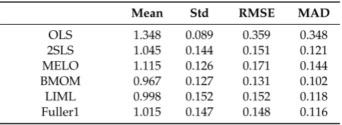
Table 1.T=50,ρ=0.60,k2=4, R2=0.40.

Mean Std RMSE MAD

OLS 1.348 0.089 0.359 0.348

2SLS 1.045 0.144 0.151 0.121

MELO 1.115 0.126 0.171 0.144

BMOM 0.967 0.127 0.131 0.102

LIML 0.998 0.152 0.152 0.118

Fuller1 1.015 0.147 0.148 0.116

12 _{We found that the median-bias and dispersion of the posterior density of}_β_{from the}_Geweke₍₁₉₉₆_{) approach increase as}_τ2 gets larger. Although one might suspect that the convergence the Gibbs sampler could be slow with smaller values ofτ2_, our convergence diagnostics did confirm this concern.

(14)

Table 1.Cont.

Fuller4 1.061 0.136 0.149 0.120

JIVE 0.957 0.178 0.183 0.141

Geweke_Mode 1.056 0.140 0.151 0.122

Geweke_Median 1.031 0.143 0.146 0.116

LIML_GS_Mode 1.061 0.139 0.152 0.123

LIML_GS_Median 1.036 0.142 0.146 0.116

CP_Mode 1.046 0.144 0.151 0.121

CP_Median 1.021 0.145 0.147 0.115

KVD_Mode 1.090 0.148 0.173 0.143

KVD_Median 1.079 0.137 0.158 0.130

Notes: Number of replications: 400. Geweke: nburn=100, n=2000. CP: nburn_GS=100, nburn_MH=100, n=5000, acceptance rate=0.482 (0.015). KVD: nburn_GS=100, nburn_MH=100, n=4000, acceptance rate=0.215 (0.136).

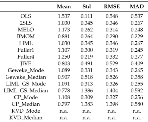
Table 2.T=50,ρ=0.60,k2=1, R2=0.10.

OLS 1.537 0.111 0.548 0.537

2SLS 1.030 0.345 0.346 0.267

MELO 1.173 0.262 0.314 0.248

BMOM 0.881 0.264 0.290 0.229

LIML 1.030 0.345 0.346 0.267

Fuller1 1.107 0.300 0.319 0.245

Fuller4 1.250 0.219 0.332 0.277

JIVE 0.803 0.491 0.529 0.409

Geweke_Mode 1.089 0.331 0.343 0.265

Geweke_Median 0.907 0.518 0.526 0.358

LIML_GS_Mode 1.091 0.313 0.326 0.255

LIML_GS_Median 0.778 1.386 1.404 0.592

CP_Mode 1.108 0.309 0.327 0.256

CP_Median 0.797 1.383 1.398 0.580

KVD_Mode n.a. n.a. n.a. n.a.

KVD_Median n.a. n.a. n.a. n.a.

Notes: Number of replications: 400. Geweke: nburn=100, n=3000. CP: nburn_GS=200, nburn_MH=200, n=10,000, acceptance rate=0.551 (0.023).

Table 3.T=50,ρ=0.60,k2=4, R2=0.10.

OLS 1.539 0.111 0.550 0.539

2SLS 1.231 0.279 0.362 0.296

MELO 1.366 0.186 0.411 0.368

BMOM 0.943 0.184 0.193 0.154

LIML 1.043 0.579 0.581 0.386

Fuller1 1.143 0.367 0.394 0.307

Fuller4 1.281 0.244 0.372 0.307

JIVE 0.816 0.568 0.597 0.474

Geweke_Mode 1.244 0.287 0.377 0.309

Geweke_Median 1.204 0.309 0.370 0.300

LIML_GS_Mode 1.260 0.268 0.373 0.308

LIML_GS_Median 1.220 0.298 0.370 0.300

CP_Mode 1.230 0.293 0.372 0.301

(15)

Table 3.Cont.

KVD_Mode 1.351 0.384 0.520 0.389

KVD_Median 1.381 0.367 0.529 0.405

Notes: Number of replications: 400. Geweke: nburn=100, n=2000. CP: nburn_GS=100, nburn_MH=100, n=10,000, acceptance rate=0.475 (0.010). KVD: nburn_GS=100, nburn_MH=100, n=3000, acceptance rate=0.400 (0.217).

Table 4.T=50,ρ=0.60,k2=9, R2=0.10.

OLS 1.535 0.111 0.546 0.535

2SLS 1.363 0.221 0.425 0.371

MELO 1.463 0.139 0.483 0.463

BMOM 0.969 0.132 0.136 0.106

LIML 1.090 0.864 0.869 0.534

Fuller1 1.182 0.479 0.512 0.366

Fuller4 1.302 0.291 0.419 0.333

JIVE 0.706 0.933 0.978 0.728

Geweke_Mode 1.357 0.239 0.430 0.367

Geweke_Median 1.350 0.245 0.427 0.361

LIML_GS_Mode 1.375 0.218 0.328 0.380

LIML_GS_Median 1.367 0.228 0.432 0.374

CP_Mode 1.215 0.629 0.665 0.466

CP_Median 1.255 0.388 0.464 0.346

KVD_Mode 1.550 0.376 0.666 0.556

KVD_Median 1.573 0.322 0.657 0.576

Notes: Number of replications: 400. Geweke: nburn=100, n=1000. CP: nburn_GS=200, nburn_MH=200, n=10,000, acceptance rate=0.242 (0.040). KVD: nburn_GS=200, nburn_MH=100, n=10,000, acceptance rate=0.267 (0.188).

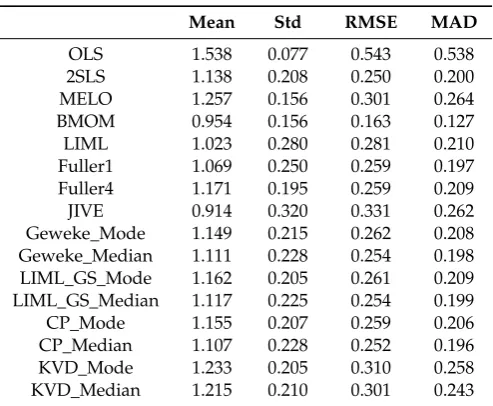
Table 5.T=100,ρ=0.60,k2=4, R2=0.10.

OLS 1.538 0.077 0.543 0.538

2SLS 1.138 0.208 0.250 0.200

MELO 1.257 0.156 0.301 0.264

BMOM 0.954 0.156 0.163 0.127

LIML 1.023 0.280 0.281 0.210

Fuller1 1.069 0.250 0.259 0.197

Fuller4 1.171 0.195 0.259 0.209

JIVE 0.914 0.320 0.331 0.262

Geweke_Mode 1.149 0.215 0.262 0.208

Geweke_Median 1.111 0.228 0.254 0.198

LIML_GS_Mode 1.162 0.205 0.261 0.209

LIML_GS_Median 1.117 0.225 0.254 0.199

CP_Mode 1.155 0.207 0.259 0.206

CP_Median 1.107 0.228 0.252 0.196

KVD_Mode 1.233 0.205 0.310 0.258

KVD_Median 1.215 0.210 0.301 0.243

(16)

Table 6.T=100,ρ=0.60,k2=9, R2=0.10.

OLS 1.542 0.078 0.548 0.542

2SLS 1.258 0.197 0.325 0.274

MELO 1.376 0.134 0.399 0.376

BMOM 0.972 0.132 0.135 0.110

LIML 1.003 0.437 0.437 0.291

Fuller1 1.071 0.311 0.319 0.243

Fuller4 1.180 0.233 0.294 0.232

JIVE 0.927 0.408 0.414 0.333

Geweke_Mode 1.253 0.201 0.323 0.269

Geweke_Median 1.238 0.206 0.315 0.261

LIML_GS_Mode 1.265 0.196 0.330 0.278

LIML_GS_Median 1.247 0.202 0.319 0.266

CP_Mode 1.196 0.264 0.329 0.266

CP_Median 1.192 0.232 0.301 0.240

KVD_Mode 1.371 0.278 0.464 0.382

KVD_Median 1.395 0.269 0.478 0.397

Notes: Number of replications: 400. Geweke: nburn=100, n=1000. CP: nburn_GS=200, nburn_MH=200, n=6000, acceptance rate=0.434 (0.029). KVD: nburn_GS=200, nburn_MH=200, n=10,000, acceptance rate=0.210 (0.179).

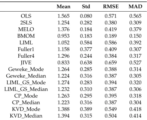
Table 7.T=100,ρ=0.60,k2=4, R2=0.05.

OLS 1.565 0.080 0.571 0.565

2SLS 1.254 0.282 0.380 0.309

MELO 1.376 0.184 0.419 0.379

BMOM 0.953 0.183 0.189 0.150

LIML 1.052 0.584 0.586 0.392

Fuller1 1.158 0.377 0.409 0.307

Fuller4 1.296 0.244 0.384 0.317

JIVE 0.833 0.638 0.659 0.527

Geweke_Mode 1.264 0.285 0.388 0.314

Geweke_Median 1.224 0.316 0.387 0.305

LIML_GS_Mode 1.274 0.283 0.394 0.320

LIML_GS_Median 1.232 0.310 0.387 0.306

CP_Mode 1.263 0.295 0.395 0.318

CP_Median 1.223 0.316 0.387 0.304

KVD_Mode 1.388 0.389 0.549 0.418

KVD_Median 1.394 0.315 0.504 0.414

Table 8.T=100,ρ=0.60,k2=9, R2=0.05.

OLS 1.574 0.076 0.579 0.574

2SLS 1.386 0.219 0.444 0.394

MELO 1.478 0.131 0.496 0.478

BMOM 0.979 0.129 0.131 0.105

LIML 1.139 0.882 0.893 0.545

Fuller1 1.224 0.477 0.527 0.389

Fuller4 1.335 0.280 0.437 0.358

JIVE 0.844 0.823 0.838 0.663

Geweke_Mode 1.385 0.243 0.455 0.395

(17)

Table 8.Cont.

LIML_GS_Mode 1.397 0.230 0.459 0.404

LIML_GS_Median 1.387 0.236 0.453 0.396

CP_Mode 1.338 0.465 0.575 0.433

CP_Median 1.337 0.311 0.459 0.376

KVD_Mode 1.584 0.462 0.745 0.592

KVD_Median 1.608 0.368 0.711 0.610

Table 9.T=100,ρ=0.20,k2=4, R2=0.10.

OLS 1.172 0.090 0.194 0.174

2SLS 1.046 0.253 0.257 0.206

MELO 1.083 0.189 0.206 0.164

BMOM 0.859 0.190 0.237 0.195

LIML 1.017 0.333 0.333 0.260

Fuller1 1.029 0.298 0.299 0.236

Fuller4 1.059 0.235 0.242 0.192

JIVE 0.957 0.417 0.419 0.340

Geweke_Mode 1.053 0.251 0.257 0.200

Geweke_Median 1.041 0.267 0.270 0.214

LIML_GS_Mode 1.058 0.244 0.251 0.197

LIML_GS_Median 1.044 0.265 0.269 0.212

CP_Mode 1.054 0.255 0.261 0.205

CP_Median 1.040 0.271 0.274 0.218

KVD_Mode 1.131 0.368 0.391 0.237

KVD_Median 1.161 0.328 0.365 0.245

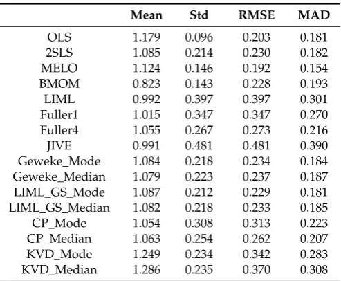
Table 10.T=100,ρ=0.20,k2=9, R2=0.10.

OLS 1.179 0.096 0.203 0.181

2SLS 1.085 0.214 0.230 0.182

MELO 1.124 0.146 0.192 0.154

BMOM 0.823 0.143 0.228 0.193

LIML 0.992 0.397 0.397 0.301

Fuller1 1.015 0.347 0.347 0.270

Fuller4 1.055 0.267 0.273 0.216

JIVE 0.991 0.481 0.481 0.390

Geweke_Mode 1.084 0.218 0.234 0.184

Geweke_Median 1.079 0.223 0.237 0.187

LIML_GS_Mode 1.087 0.212 0.229 0.181

LIML_GS_Median 1.082 0.218 0.233 0.185

CP_Mode 1.054 0.308 0.313 0.223

CP_Median 1.063 0.254 0.262 0.207

KVD_Mode 1.249 0.234 0.342 0.283

KVD_Median 1.286 0.235 0.370 0.308

(18)

Table 11.T=50,ρ=0.95,k2=4, R2=0.10.

OLS 1.846 0.052 0.848 0.846

2SLS 1.359 0.180 0.402 0.363

MELO 1.572 0.118 0.584 0.572

BMOM 1.057 0.118 0.131 0.102

LIML 0.988 0.404 0.404 0.255

Fuller1 1.169 0.196 0.259 0.221

Fuller4 1.417 0.120 0.434 0.417

JIVE 0.637 0.611 0.711 0.478

Geweke_Mode 1.347 0.302 0.460 0.358

Geweke_Median 1.277 0.377 0.468 0.305

LIML_GS_Mode 1.338 0.155 0.372 0.345

LIML_GS_Median 1.252 0.194 0.318 0.281

CP_Mode 1.314 0.162 0.353 0.325

CP_Median 1.234 0.194 0.304 0.266

KVD_Mode 1.411 0.379 0.559 0.428

KVD_Median 1.462 0.463 0.654 0.514

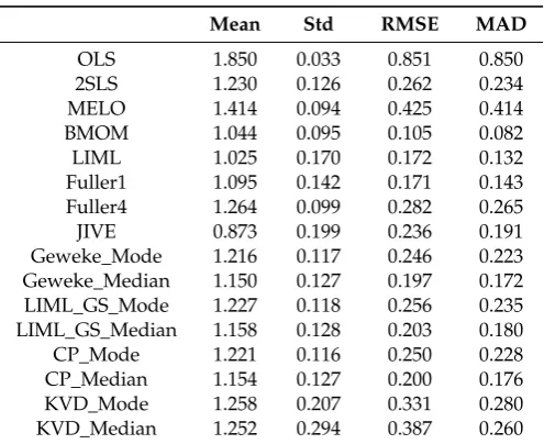
Table 12.T=100,ρ=0.95,k2=4, R2=0.10.

OLS 1.850 0.033 0.851 0.850

2SLS 1.230 0.126 0.262 0.234

MELO 1.414 0.094 0.425 0.414

BMOM 1.044 0.095 0.105 0.082

LIML 1.025 0.170 0.172 0.132

Fuller1 1.095 0.142 0.171 0.143

Fuller4 1.264 0.099 0.282 0.265

JIVE 0.873 0.199 0.236 0.191

Geweke_Mode 1.216 0.117 0.246 0.223

Geweke_Median 1.150 0.127 0.197 0.172

LIML_GS_Mode 1.227 0.118 0.256 0.235

LIML_GS_Median 1.158 0.128 0.203 0.180

CP_Mode 1.221 0.116 0.250 0.228

CP_Median 1.154 0.127 0.200 0.176

KVD_Mode 1.258 0.207 0.331 0.280

KVD_Median 1.252 0.294 0.387 0.260

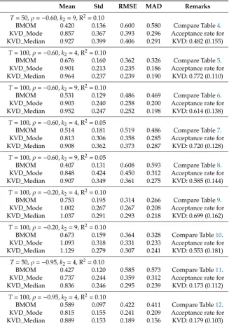
Table 13.Performance of BMOM and KVD whenρ<0.

Mean Std RMSE MAD Remarks

T=50,ρ=−_0.60,_k₂=_{4, R}2=_0.40

BMOM 0.852 0.129 0.196 0.165 Compare Table1.

KVD_Mode 0.971 0.150 0.152 0.119 Acceptance rate for

KVD_Median 0.999 0.153 0.152 0.119 KVD: 0.713 (0.130)

T=50,ρ=−_0.60,_k₂=_{4, R}2₌_0.10

(19)

Table 13.Cont.

Mean Std RMSE MAD Remarks

T=50,ρ=−_0.60,_k₂=_{9, R}2=_0.10

KVD_Median 0.927 0.399 0.406 0.291 KVD: 0.482 (0.155)

T=100,ρ=−_0.60,_k₂=_{4, R}2=_0.10

KVD_Median 0.964 0.237 0.239 0.190 KVD: 0.772 (0.110)

T=100,ρ=−_0.60,_k₂=_{9, R}2=_0.10

KVD_Median 0.952 0.247 0.252 0.198 KVD: 0.614 (0.138)

T=100,ρ=−_0.60,_k₂=_{4, R}2=_0.05

KVD_Median 0.908 0.362 0.373 0.287 KVD: 0.720 (0.128)

T=100,ρ=−_0.60,_k₂=_{9, R}2₌_0.05

KVD_Median 0.907 0.349 0.361 0.275 KVD: 0.585 (0.144)

T=100,ρ=−_0.20,_k₂=_{4, R}2₌_0.10

KVD_Median 1.037 0.291 0.293 0.218 KVD: 0.699 (0.162)

T=100,ρ=−_0.20,_k₂=_{9, R}2=_0.10

KVD_Median 1.129 0.279 0.307 0.241 KVD: 0.553 (0.181)

T=50,ρ=−_0.95,_k₂=_{4, R}2=_0.10

KVD_Median 0.836 0.246 0.295 0.239 KVD: 0.173 (0.112)

T=100,ρ=−_0.95,_k₂=_{4, R}2=_0.10

KVD_Median 0.889 0.153 0.189 0.156 KVD: 0.179 (0.103)

Notes: Number of replications: 500.

Table13summarizes the results for cases withρ <0 for BMOM and KVD for whom negative

ρmade a surprising difference. As mentioned before, we focus on the estimates of the structural parameter β. Specifically, we analyze the sensitivity of the various estimates ofβwith respect to the strength of the instrumental variables Z, the degree of overidentification(k2−_m₊₁₎_{, the degree}

(20)

an estimator is symmetric with respect to the sign of parameterρ, an issue generally overlooked in the literature.14

Note that the strength of the instrumental variables for the included endogenous variable Y2is measured in terms of the adjusted R2by regressingY2onZ=(Z1,Z2). In the data generating process, we controlled R2to be within±_{2.5% of the specified value to reduce unnecessary variation. We did not}

experiment with extremely small R2(say, 0.01 or less). In these cases, the mean values of all estimators approached the point of concentrationω12/ω22, which is equal to(β+ρ)for our data generating process (DGP).

For each specification, the number of replications is 400. The number of burn-ins (nburn_GS and nburn_MH), and subsequent number of iterations (n) determined at the convergence diagnosis step are reported in the footnotes to each table.

The average acceptance rate and its standard deviation (in parentheses) across replications for each M–H routine are reported as well. To evaluate alternative estimators, we computed mean, standard deviation (Std), root of mean squared errors (RMSE), and mean absolute deviation (MAD) over repeated experiments for all the estimators considered.15 Since LIML, posterior densities for CP and KVD, as well as 2SLS in the just-identified case do not have finite moments of positive order in finite samples, one should interpret the computed mean, standard deviation and RMSE across replications for these estimators with caution. In this sense, the MAD across replications is a preferred measure to consider.

We will first look at cases reported in Tables1–12withρ > 0. In Table1, we consider a case (T=50,

ρ=0.60,k2=4) with moderately strong instruments (R2=0.40). It is found that with reasonably strong instruments all estimators designed for simultaneous equations perform reasonably well. As expected, OLS is seriously biased. BMOM has a slight edge over others in terms of RMSE and MAD. For all Bayesian approaches and LIML-GS, the medians perform a little better than modes, and CP over KVD, in terms of bias, RMSE, and MAD. Notice that the classical LIML estimates are different from LIML-GS (mode or median). As noted byDrèze(1976), from a Bayesian viewpoint, LIML produces an estimate ofβconditionally on the overidentifying restrictions, the modal values of all the remaining parameters, and a uniform prior. In other words, the concentrated likelihood function ofβafter concentrating out (i.e., maximizing with respect to) other reduced-form and nuisance parameters is a conditional density. However, LIML-GS is a marginal density with all other parameters being integrated out. Due to possible asymmetry in the distribution of the nuisance parameters, the modal/median values of LIML-GS may not coincide with classical LIML estimates. In all our experiments, we find that the median-unbiasedness property of (conditional) LIML does not carry over to the marginal LIML (i.e., LIML-GS); however, the former generally has a much larger standard deviation than the latter. In a way, LIML-GS brings the classical LIML estimator close to its Bayesian counterpart for the purpose of comparison.

It is interesting to note that across all our tables, the difference between LIML-GS and CP can only be attributed to the importance of Jeffreys prior. Compared to LIML-GS, typically CP has a smaller bias, but slightly larger standard deviation, even though the differences are very small. In some cases,

14 _Denote_Ω₌

"

ω11 ω12 ω12 ω22

#

. UsingΣ=C0ΩC, we haveσ12=ω11−2βω12+β2ω22,σ12=ω12−βω22, andσ22=ω22. Lettingρ=σ12/

√

σ11σ22, the second relationship may be rewritten as:

β−ω12 ω22

=−ρ r

σ11 ω22

IfΣis normalized as in (35) withσ11=ω22=1, thenω12=β+ρ. Therefore, in our context, givenβ=1, the sign and magnitude ofρ(orω12) has a special significance.

(21)

however, the use of Jeffreys prior reduces the bias in CP quite substantially. For example, in Table4 withT=50 and a high degree of overidentification, the bias is reduced from 0.36 to 0.25.

A simple case when the structural model is just identified (k2=1) is reported in Table2. For this case it is well known that classical LIML coincides with 2SLS. The KVD approach does not accommodate the case of just-identification since (15) requiresk2>(m−1).16 In this case, we find that CP-Mode produces results closer to LIML-GS-Mode than to LIML. CP (1998) showed that for a two-equation just-identified SEM in orthonormal canonical form, the posterior density ofβwith Jeffreys prior has precisely the same functional form as the density of the finite sample distribution of the corresponding LIML estimator as obtained byMariano and McDonald(1979). Our simulation results show that the assumption of orthonormal canonical form is crucial for their exact correspondence, which cannot be extended to a general SEM.17 In general, the Bayesian marginal density is not the same as the classical conditional density. Interestingly, JIVE is considerably more biased and has larger standard deviation than 2SLS. Also, CP-Median and LIML-GS-Median perform significantly worse than their modes. This is because in an exactly identified model with weak instruments, the probability of local nonidentification is substantial, and the resulting nonstandard marginal density exhibits a very high variance. The same result holds true for Geweke-Median, but to a lesser extent. Thus, for exactly identified SEMs with very weak instruments, mode of the marginal density is a more dependable measure ofβ. We should point out that in all other cases in this study, the medians generally turned out to be more preferable than the modes in terms of bias, RMSE, and MAD (see Tables11and12, for instance).

Results reported in Tables 3–12 consider cases with general overidentification and weak instruments. As noted in the literature, OLS and 2SLS are median-biased in the direction of the correlation coefficientρ, and the bias in 2SLS grows with the degree of over identification, and decreases as sample size increases. Results in Tables3–10confirm these results. Since MELO is a single K-class estimator with 0<K<1, its performance is always between OLS and 2SLS estimates. The bias in MELO shows the same pattern as that of 2SLS. With moderate simultaneity, the median-bias in 2SLS can be as large as about 40% of the true value (see Table8). We note that MELO, LIML-GS-Mode, and KVD-Mode or KVD-Median are also median-biased in the direction ofρ. However, the bias in JIVE is consistently in the opposite direction ofρ. Classical LIML is remarkably median-unbiased when the instrumental variables are not very weak, which is well documented in the literature. We find that LIML is median-biased in the direction ofρwhen the instruments are very weak (Table8), which is consistent with the finding inStaiger and Stock(1997) using local-to-zero asymptotic theory. Even in this situation, the bias of LIML is much smaller than that of any other estimator, except BMOM.

The MAD of OLS is very close to its bias (i.e., relatively small Std) across all cases and it implies that OLS method is robust in the sense that it does not suffer from heavy tails or outlying estimates, seeZellner(1998). In this sense, MELO and BMOM are all robust with relatively small standard deviations across replications. However, OLS exhibits large bias in the presence of simultaneity and is not so appealing. It is known that for a degree of overidentification strictly less than seven, 2SLS would have a smaller asymptotic mean squared error (AMSE) than LIML, cf. Mariano and McDonald

16 _When_k

2=(m−1), a diffuse prior in (20) for the linear model implies that the prior for the parameters of the LISEM (4) is

p(β,π1,Π1,Π2,Ω)∝ |Ω|

−(k+m+1)/2_|_Π 2|,

and the prior for the parameters of the LISEM (1) and (2) is

p(β,γ,Π1,Π2,Σ)∝ |Σ|

−(k+m+1)/2_|_Π 2|

which is identical to the Jeffreys prior; see also expressions (22) and (42) in CP.

(22)

(1979) and references therein. In cases with weak instruments the situation gets more complicated in finite samples. In our experiments, LIML has larger RMSE and MAD than 2SLS except in Tables11 and12whereρwas 0.95. Note that the degree of overidentification is 8.0 in Tables4,6,8and10.

Among classical estimators, JIVE turns out to be least appealing. Monte Carlo simulations in Angrist et al. (1999) showed that JIVE has slight median bias in the opposite direction ofρ(but less than 2SLS) and have heavier tails than LIML. Our Table6is comparable to panel 2 of their Table1, and the results are similar. Our other experiments show that JIVE may also have large absolute bias (larger than LIML) in the case with weak instruments, sometimes even greater than 2SLS (see Table2). Generally, JIVE has slightly less bias than 2SLS, but this gain is overshadowed by enlarged standard deviation such that in finite samples it has no advantage over 2SLS in terms of MAD and RMSE. We also find that JIVE has greater RMSE and MAD than LIML.Blomquist and Dahlberg(1999) experimented with much larger sample sizes than ours. Comparing our Table4with Table6and with an unreported simulation with a sample size of 500, we found that the relative gain in JIVE is more than other estimators as sample size increases, even though its relative low standing remains valid. Examined from different angles, these results are very similar to those reported byDavidson and MacKinnon(2006a,2006b).18 Fuller’s modified LIML estimators are included because Fuller1 is designed to minimize the median-bias, and Fuller4 to minimize the mean-squared error. It seems that this conclusion is also problematic in the presence of weak instruments. Between the two, Fuller1 has smaller median-bias, and Fuller4 has smaller standard deviations across replications. However, in terms of RMSE or MAD, Fuller4 shows no advantage over Fuller1 in most of the cases.

Because all the estimators except OLS are consistent and their asymptotic distributions are also the same, results in Tables3–6confirm that their bias and dispersion decrease as sample size increases. But if the instruments are very weak (see Tables7and8), their bias and dispersion may remain significant, a point emphasized forcefully byZellner(1998). However, when the endogeneity is not strong (see Tables9and10), their bias and dispersion may not be a big concern for some of the estimators.

Across all cases, we find that the bias in BMOM is small if ρ is not too small and the structural Equation (1) is overidentified. As sample size increases or degree of over-identification rises, the observed bias in BMOM decreases. The most striking feature of BMOM is that it exhibits the smallest MAD and Std whenρis not too small. MELO shows slightly smaller MAD and Std than BMOM ifρis small (see Tables9and10). In cases with very weak instruments and a high degree of overidentification, the MAD of BMOM is only one-fourth of that of other estimators (see Table8). These are in accordance withTsurumi(1990)’s finding that in many cases, ZEM has the least relative mean absolute deviation. Meanwhile, ifρis very small and the structural equation is overidentified, the bias in BMOM can be large; 2SLS, LIML-GS, Geweke, and CP perform remarkably well in these situations.

Next, we examine in more detail the performance of the Bayesian approaches. Overall, the median bias resulting from these approaches exhibits the same pattern as the bias of 2SLS, it increases with the degree of overidentification, and decreases as sample size rises. TheGeweke(1996) approach used a shrinkage prior but its performance is comparable with LIML-GS and CP. The median-bias from PMOD-Geweke is the same or slightly less than that of LIML-GS-Mode, and the bias from Geweke-Median is always slightly less than that of LIML-GS-Median. Similar relationships are observed for MADs. These reflect the impact of the (informative) shrinkage prior on the posterior density.

For each specification, the acceptance rate in the M–H algorithm using CP approach is stable while that using KVD approach shows huge variation across replications. The acceptance rate for CP is generally above 40%, except when sample size is small and the degree of overidentification is high. This shows that the posterior of CP is largely dominated by the likelihood function (3) and the Jeffreys