retrieval and validation results
F. Azam1, K. Bramstedt1, A. Rozanov1, K. Weigel1, H. Bovensmann1, G. P. Stiller2, and J. P. Burrows1 1Institute of Environmental Physics – IUP, University of Bremen, Bremen, Germany
2Institute for Meteorology and Climate Research – IMK, Karlsruhe Institute of Technology – KIT, Karlsruhe, Germany
Correspondence to: F. Azam (faiza@iup.physik.uni-bremen.de)
Received: 31 October 2011 – Published in Atmos. Meas. Tech. Discuss.: 3 February 2012 Revised: 31 August 2012 – Accepted: 3 September 2012 – Published: 24 October 2012
Abstract. SCIAMACHY (SCanning Imaging Absorption spectroMeter for Atmospheric CHartographY) lunar occulta-tion measurements have been used to derive vertical profiles of stratospheric water vapor for the Southern Hemisphere in the near infrared (NIR) spectral range of 1350–1420 nm. The focus of this study is to present the retrieval method-ology including the sensitivity studies and optimizations for the implementation of the radiative transfer model on SCIA-MACHY lunar occultation measurements. The study also in-cludes the validation of the data product with the collocated measurements from two satellite occultation instruments and two instruments measuring in limb geometry. The SCIA-MACHY lunar occultation water vapor measurement com-parisons with the ACE-FTS (Atmospheric Chemistry Ex-periment Fourier Transform Spectrometer) instrument have shown an agreement of 5 % on the average that is well within the reported biases of ACE in the stratosphere. The compar-isons with HALOE (Halogen Occultation Experiment) have also shown good results where the agreement between the instruments is within 5 %. The validations of the lunar oc-cultation water vapor measurements with MLS (Microwave Limb Sounder) instrument are exceptionally good, varying between 1.5 to around 4 %. The validations with MIPAS (Michelson Interferometer for Passive Atmospheric Sound-ing) are in the range of 10 %. A validated dataset of water vapor vertical distributions from SCIAMACHY lunar occul-tation measurements is expected to facilitate the understand-ing of physical and chemical processes in the southern mid-latitudes and the dynamical processes related to the polar vortex.
1 Introduction
SCIAMACHY (SCanning Imaging Absorption spectroMe-ter for Atmospheric CHartographY) (Burrows et al., 1995) is a moderate resolution 8-channel grating spectrometer on-board Envisat, launched in 2002. The instrument mea-sures solar irradiances and the earthshine radiances from the UV to the NIR (near infrared) (240–2380 nm) spec-tral region in nadir, limb and solar/lunar occultation geome-try. SCIAMACHY is dedicated to improving our knowledge in atmospheric composition and global atmospheric change (Bovensmann et al., 1999). Since the launch of its host satel-lite, the instrument has provided total columns as well as vertical profiles of atmospheric parameters relevant to ozone chemistry, air pollution and global climate change issues, from the troposphere up to the mesosphere (Gottwald and Bovensmann, 2011).
SCIAMACHY lunar occultation measurements have pro-vided valuable datasets of atmospheric species, as ozone, ni-trate radical and nitrogen dioxide (Amekudzi et al., 2005, 2009), which have been used for physical and chemical in-terpretations and analysis.
tropopause. However, this has to pass through the cold trap of the temperature minimum at the tropopause region; above this region the oxidation of methane and other hydrocarbons release hydrogen containing free radicals with H2O being formed by the reaction with OH. Thus, very low water va-por amounts are found in the tropical lower stratosphere due to the air ascending through the cold tropical tropopause re-gion with an annual average of around 3.8 ppmv (Dessler and Kim, 1999). In the upper stratosphere, methane oxida-tion is the dominant local stratospheric water vapor source (Abbas et al., 1996; Michelsen et al., 2000), and the relation-ship between stratospheric methane and water vapor has been demonstrated in previous studies (Gurlit et al., 2005). Higher water vapor mixing ratios are observed with increasing alti-tude reaching around 7 ppmv near the stratopause (Pan et al., 2002). The large scale general circulation across the hemi-spheres brings the moist air into the polar region where it descends inside the polar vortex. In the polar stratosphere, the water vapor amounts remain high with the exception of the dehydration events in the polar lower stratosphere due to the formation of polar stratospheric clouds (PSCs). In-side the polar vortex, the water vapor amounts directly influ-ence the ozone depletion by controlling the formation tem-peratures, the size of the polar stratospheric clouds (Kirk-Davidoff et al., 1999; Kirk-(Kirk-Davidoff and Lamarque, 2008), and the polar vortex temperatures.
SCIAMACHY’s measurements in the occultation mode are self calibrating and have high accuracy. This feature also makes them well suited for the trend analysis. The measure-ments give localized coverage where the vertical profiles of stratospheric constituents are retrieved with a vertical resolu-tion of 3–4 km.
2 SCIAMACHY lunar occultation
SCIAMACHY lunar occultation measurements are carried out over the southern high latitudes between 59–89◦S dur-ing local nighttime, and the measurements from 2002 to 2010 are used in this study. The latitudinal constraint is due to the sun synchronous orbit of Envisat and the placement of the in-strument on the satellite. The SCIAMACHY’s field of view (FOV) in lunar occultation mode is 0.045◦ (2.5 km) in the vertical direction and 1.8◦ in the horizontal direction. The apparent diameter of the moon is between 0.49◦ and 0.57◦ in the horizontal direction, which is within the instrument’s FOV. The properties of moonrise in SCIAMACHY’s FOV are determined by the orientation of the lunar orbital plane with respect to Envisat’s orbital plane and the ecliptic. Each measurement starts when the moon rises above a tangent height altitude of around 17.2 km. Below this altitude, the lunar signal is rapidly decreasing. The scanner follows the predicted movement of the moon for 16 s, then the moon fol-lower device (MFD) takes over and adjusts the scanner to the brightest point of the moon. The switch is at an altitude
of about 65 km. Above 100 km, the measurements are per-formed for calibration purposes and to calculate transmis-sion. The moonrise is observed when the phase is>0.5 in the instrument’s FOV with solar zenith angle (SZA)>94◦. The measurements end shortly after the full moon.
In the southern polar region, the polar night lasts from April till September. The winter season spans from June to September. The months of July, August and September en-dure the coldest temperatures. During this period, the het-erogeneous chemistry on the surface of PSCs kicks off the formation of the ozone hole. As originally proposed, SCIA-MACHY comprised two instruments for limb and nadir. As a result of cost reduction imposed by the space agencies, the instrumentation aboard Envisat in its sun synchronous orbit comprises a single instrument, undertaking solar occultation in the Northern Hemisphere, alternate but matched limb and nadir during an orbit, and lunar occultation in the Southern Hemisphere. On the average, the yearly SCIAMACHY lu-nar occultation measurements extend from November to June owing to the limitations described above. Occasionally there are a few measurements in October. The pattern implies that the atmospheric species participating in the heterogeneous chemistry and chemical processes at high latitudes cannot be observed by these measurements. In the southern polar stratosphere, the formation of the vortex begins to spin up in March, and, as a result of momentum transport to high lati-tudes, it breaks down typically in November or December. The quantitative analysis of water vapor distributions and variability in the polar stratosphere provides a perspective into the evolution and the break down of the polar vortex. The strong relationship between water vapor and the upper at-mospheric dynamics has been established in various studies (Russell et al., 1993a; Lahoz et al., 1993, 1996). The retrieval of stratospheric water vapor from SCIAMACHY lunar oc-cultation measurements yields some unique insight into the dynamics of the stratosphere and provides the motivation be-hind the study.
3 Solar zenith angle and the moon phase distribution for the lunar occultation measurements
Fig. 1. SCIAMACHY lunar occultation tangent points in 2010; the
latitudes vary within 59◦S–89◦S.
Fig. 2. SCIAMACHY lunar occultation latitudinal distribution for
the years 2003–2010; each year the latitudes vary considerably be-tween 59◦S–89◦S.
The yearly time series of solar zenith angle (SZA) and moon phase for SCIAMACHY lunar occultation measure-ments are shown in Figs. 3 and 4, respectively. The SZA variation for each year is between 94◦ and 115◦, with the highest values observed around April. The observed moon phase values vary around 0.5–0.99. The assignment of phase is as follows: For the half moon, the phase is 0.5, and so on. The smaller the SZA value, the higher is the influence of the sunlight scattered due to the Earth’s atmosphere, whereas
Fig. 3. SCIAMACHY lunar occultation SZA distribution for the
years 2003–2010; each year the SZA span is within 94◦and 115◦.
Fig. 4. SCIAMACHY lunar occultation moon phase distribution for
the years 2003–2010; the observed moon phase values vary around 0.5–0.99.
4 Retrieval theory
This section explains the retrieval method implied on the SCIAMACHY lunar occultation measurements. The scheme is explained in depth in Amekudzi (2005) and the references therein, and will be described here in brief with emphasis on the theory that is essential to understand the contents of Sect. 5. The basic equation to be solved is a nonlinear, ill-posed inverse problem (Rodgers, 2000),
y =F (x, b)+ε, (1)
relating the measurement vectory, i.e. the measured lunar spectrum, by a forward modelF. The state vector x repre-sents the water vapor vertical profile to be estimated. The forward modelF accounts for the physics of the measure-ment including the instrumeasure-ment characterization. The vectorb includes the model parameters such as line strength, pressure broadening, temperature etc. The symbolεrepresents errors of all kinds. Equation (1) is linearized with respect to a refer-ence state signifying the first estimate of the true atmospheric state, termed as the a priorixa. The a priori is introduced by a climatology. The linearization is performed by using the Taylor series expansion and neglecting its higher terms:
y =F (xa)+
∂F (x)
∂x |xa(x−xa)+ε, (2)
where the differential on the right hand side is the weighting function matrix taking into account the sensitivity of the mea-surement to the true profile. It is denoted by K, K≈∂y/∂x. Thus
ˆ
y =y−ya =Kxˆ +ε=K(x −xa)+ε (3) relates the measurement state vectoryˆ and the model state vectorx;ˆ ya is the simulated a priori spectra. The retrieval solution is obtained by applying the optimal estimation and using the Newton iterative scheme as described in Rodgers (2000), which, for an (i+ 1)-th step, results in
xi+1=xa+
KTi S−y1Ki +S−a1
−1
KTi S−y1(y−yi+Ki(xi −xa)) , (4) with Sa as the constraint matrix for the state vector called a priori covariance matrix, reflecting uncertainties of the a priori height profiles, and Sy as the measurement error co-variance matrix representing the measurement noise for ev-ery measurement height and wavelength. In this study, 100 % a priori covariance is assumed. In Eq. (4),
Di =
KTi S−y1Ki +S−a1
−1
KTi S−y1 (5)
is the contribution function representing the sensitivity of the retrieval to the measurement, implying D≈∂xˆ/∂y. The convergence to terminate the iterations is achieved when the
measurement residualsyi−yare sufficiently small or the re-trieved profile does not change anymore during the iterations. Inverse problems in general are sensitive to small pertur-bations that may introduce unrealistic features. In our study, the inversion was stabilized by using an optimization ap-proach which suppresses the additive noise. A regularization term called the Tikhonov regularization (Tikhonov, 1963; Tikhonov and Arsenin, 1997) was introduced in the retrieval solution by extending the inverse of the a priori covariance matrix by a Tikhonov matrix as
S−a1−→Sa−1+STt St. (6)
This constrains the smoothness of the retrieved profile x,ˆ contributing to the desired state of the retrieved atmospheric parameter. In Eq. (6), St is the first order derivative matrix weighted by an appropriate parameter termed the Tikhonov parameter. An appropriate value of the Tikhonov parameter has to be selected, as will be shown in Sect. 5.4.4, minimiz-ing the loss of information.
The retrieval solution covariance matrix (smoothing error and retrieval noise) corresponding to Eq. (4) is given by
S=KTi Sy−1Ki +S−a1
−1
. (7)
The diagonal elements of S are the covariances of the re-trieved water vapor profiles and are the indicators of the the-oretical precision of the retrieval.
5 Water vapor retrieval
5.1 Data
The data used for the retrieval was the SCIAMACHY lunar occultation level 1b (l1b) data provided by ESA. The l1b data contain the measured raw spectra and all information necessary for calibration. In our study the data versions 6.03 and 7.0 were used, completing the period of 2002–2010 to derive the vertical profiles of stratospheric water vapor from ∼17–50 km in the NIR spectral region. The data version 6.03 covers 2002–2009. Starting in October 2009, the processing switched to version 7.0; reprocessing of the earlier period was not complete at the time of this study. Version 7.0 in-cludes improvements for some of the calilbration data. How-ever, for the wavelength region and the calibration steps ap-plied for this study (Sect. 5.3), the calibration data are the same in both data versions, therefore the switch in the data version has no impact.
5.2 Wavelength window
Fig. 5. Spectral plot for the wavelength window 1350–1450 nm
and 24 km tangent height: Red line is the measured water va-por differential absorption spectrum. Green line is the correspond-ing modelled differential optical depth. A strong CO2absorption line is present around 1430 nm. Wavelength section 1350–1420 nm was selected for the retrieval (Measurement: 13 March 2006, or-bit = 21 085, SZA = 109.137, moon phase = 0.93).
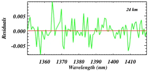
line is the modelled differential optical depth, and the red line represents the measured differential spectrum of water vapor. The attributes of the differential optical depth spectra and their calculation are described in Sect. 5.4.1. The spectral window 1350–1450 nm contains a strong absorption by CO2 around 1430 nm. To obviate any complexity arising from the exponential sum fitting of transmission (ESFT) coefficients approximation radiative transfer method (see Sect. 5.4) in handling two absorbers in the same window, the wavelength section 1350–1420 nm was selected as the extraction and retrieval wavelength window. A good fit was observed for 1350–1420 nm. Figure 6 shows the residual plot for the se-lected window, associated to Fig. 5, signifying the difference between the measured and the simulated differential spectra. As can be seen, the residuals are of the order of 0.5 %, which is within the signal to noise ratio.
5.3 Lunar spectrum extraction
The raw lunar radiance spectra are calibrated for offsets such as nonlinearlity, straylight and dark current correction. In ad-dition, the spectral calibration is performed. Proceeding these corrections and calibration, the lunar spectrumIj(hj, λ)or simplyIj(λ)was extracted for 13 tangent heights hj, be-tween 17–50 km, selecting the 14th at 120 km, which was the reference spectrumIref(λ). The ratio of the lunar spectrum to the reference is the transmission spectrum used. The NIR de-tectors of SCIAMACHY contain some bad pixels due to the lattice mismatch between the substrate and the light detecting material of the detector. The bad pixels may result in discon-nected pixels, different detected pixels for the same intensity, excessive noise or a very high leakage current. Two bad pix-els were identified in the wavelength region 1350–1420 nm and excluded.
Fig. 6. Residual plot for the selected wavelength window 1350–
1420 nm (corresponds to the same measurement as for Fig. 5): The residuals signify the difference between the measured and the simu-lated differential transmitted spectra. The residuals are about 0.5 %.
5.4 Retrieval methodology, sensitivity studies and optimizations
A robust and efficient inversion scheme and retrieval algo-rithm, SCIATRAN, is implemented on SCIAMACHY mea-surements for the retrieval of atmospheric parameters from the ultraviolet to near infrared region. This algorithm was de-veloped at Institute of Environmental Physics/Remote Sens-ing, University of Bremen (Rozanov, 2001), as an exten-sion of UV-Visible GOMETRAN radiative transfer model (Rozanov et al., 1997). The vertical profiles of water va-por from SCIAMACHY lunar occultation observations were retrieved using SCIATRAN version 3.0. In the framework of an optimal estimation approach, SCIATRAN is applied as a forward model, i.e. a radiative transfer model (RTM), and a retrieval code, i.e. the inverse part which fits the re-sults from the former to the real measurements. The spectral absorption line features were treated by using the exponen-tial sum fitting of transmission coefficients method (ESFT) (Sect. 5.4.3), employing correlated-kdistribution instead of the line by line (LBL) treatment of the line absorbers. The retrieval methodology for the ESFT approach is illustrated in Fig. 7.
5.4.1 Forward model/radiative transfer part
Fig. 7. SCIATRAN: setup for the retrieval by ESFT method. The functioning of forward model and the retrieval parts are elaborated here.
For the construction of the forward model, the differen-tial optical depths were considered rather than the radiances themselves (Rozanov et al., 2000, 2005). This took into ac-count the logarithm of the measured radiances. The loga-rithms increase the linearity of the inverse method applied; the increased linearity is due to the fact that the fundamen-tal physics is the transmission of the light. The logarithms thereby reduce the linearization errors (Hoogen et al., 1999; Rozanov et al., 2011). A fitted third order (low order) poly-nomialP(3) in wavelengthλwas then subtracted to reduce the effect of the broad band features. This whole approach was applied to the measured radiance at each tangent height
j, the radiance at the reference tangent height (note: both are represented by one Eq. 8) and the simulated radiances. e
Ij(λ)=lnIj(λ)−P (3) =
Ij(λ)− N=3 X
i=0
ciλi (8)
Here, c is the coefficient of the polynomial, and i is the polynomial index. Spectra of differential optical depths were used. To obtain them, the radiance spectra were divided by the reference spectrum (at 120 km altitude). This implies, numerically,
yj =
ln eIj(λ) ln Ieref(λ)
. (9)
The simulated transmission differential spectra defining the forward model were obtained in a very similar manner.
The variation or the response of the measured radiation due to the change in the vertical profile of the atmospheric parameterαk (where k is the retrieval parameter index) at a spectral point λ is mathematically termed the weighting function at the altitudehj under consideration. The weight-ing functions are elements of the matrix K, from Eq. (3), and hence are the derivatives of the measured intensityIj with respect to the relative trace gas concentrationαk,
Wjk(λ)= ∂Ij(λ)
∂αk α
k. (10)
These are the relative weighting functions and are also trans-formed to the differential form for the same reason described above. Thus
˜
Wjk = 1
Ijs(λ)W
k j −
1
Irefs (λ)W
k ref−
N=3 X
i=0
ciλi. (11)
bsq0 are the shift and squeeze parameters for the spectra at a given tangent altitude atjand at the reference height, respec-tively. This pre-processing step by SCIATRAN improved the residuals, especially for the lower stratospheric tangent heights.
5.4.2 Inversion/retrieval part
The theoretical aspects of the retrieval technique are ex-plained in Sect. 4, which involve solving the inverse prob-lem by impprob-lementation of the optimal estimation to get the desired parameter and applying Newton iterative scheme for the convergence of the solution. The retrieval procedure is sketched in Fig. 7. As shown in the figure, the retrieval can be divided into two parts. In the first part, the difference be-tween the measured and the simulated spectrum is calcu-lated. The second part takes the parameters a priori, signal to noise ratio and Tikhonov regularization and applies opti-mal estimation on the result from the former composing the vertical profile of water vapor. The optimizations related to signal to noise ratio and Tikhonov regularization parameter will be discussed in the next section. The profile obtained is fed back to the forward model section where the simula-tion and computasimula-tions are done again. A number of iterasimula-tions are carried out until the conditions described in Sect. 4 are achieved. The final retrieval profile, approximating the true atmospheric state, was obtained in this manner.
5.4.3 The line absorber treatment
As mentioned before in Sect. 5.4, the line absorber treat-ment is carried out using ESFT approximation (Wiscombe and Evans, 1977) employing correlated-kapproach and not the LBL method. The LBL radiative transfer is a monochro-matic method involving computations of radiance for each frequency in a selected wavelength window. The radiances are then integrated over this region. It should be noted that the LBL method is assumed to be a true representa-tive of the reality compared to the ESFT approximation. LBL computation has to be carried out with a sufficiently fine grid (0.001 nm/line or less) to accurately reproduce the absorption coefficient spectrum and to perform correct ra-diative transfer calculations. The LBL calculations thus re-quire substantial computing time. ESFT is preferred over LBL since it provides a good compromise between efficiency and accuracy. When LBL is used in SCIATRAN, the line
absorptions in different layers coincide spectrally. The imple-mentation of this method in SCIATRAN is discussed in de-tail in Buchwitz et al. (2000). ESFT is a fast retrieval method and its usage in SCIATRAN involves the calculation of the ESFT coefficients using HITRAN 2008 database. Mathemat-ically, in general, the absorption coefficients for simple LBL computation are given as
kλ(p, t )= X
i
Si(t ) fi(λ, p, t ), (13)
where p and t are pressure and temperature, respectively.
Si is the line intensity for the ith absorption line, and
fi(λ, p, t ) stands for the line shape factor. The spectral mean transmittance over the spectral interval1λcan be ap-proximated as
T1λ(m)= Z
1λ
exp(−kλm)
d λ
1λ, (14)
wherem is the absorber amount per unit area. In a given wavelength window, the same values ofk(p, t ) occur fre-quently. This means that the computational efficiency can be improved by replacing the integration overλin Eq. (14) by the probability distribution function of absorption coefficient
h(k), and further by their cumulative probability distribution
g(k): (Fu and Liou, 1992; Li and Barker, 2004)
T1λ(m)=
∞ Z
0
exp(−kλm)
h(k) d(k)=
1
Z
0
exp(−kgm)
d g.(15)
h(k) d kis the fraction of1λwhere the absorption coefficient value is betweenk andk+d k, and by definition g(k)is a monotonically and smoothly increasing function inkspace.
g(k)= 1 Z
0
h(k) d k (16)
Fig. 8. Number density profiles with different Tikhonov
parame-ters: The coloured lines are the retrieved water vapor profiles us-ing different Tikhonov values and the grey lines in each panel are the a priori profiles. Tihkonov parameter 3.5 was selected for the retrieval (Measurement: 13 March 2006, orbit = 21 085, SZA = 109.137, moon phase = 0.93).
absorption coefficientski(p, t )with weights wi and nodes
gi.
T1λ(m)= n X
i=0
wi
exp(−kλm)
where ki =k (gi) and X
i
wi =1 (17)
HITRAN 2008 database for ESFT implementation con-tains the spectral ranges, their corresponding line absorbers, and as explained above, the number of coefficients calculated at a number of temperature and pressure grid points for each case. As will be seen in the next section, in our study, differ-ent grids for the water vapor window 1240–1560 nm created at the Institute of Environmental Physics (IUP) were tested for the retrieval.
5.4.4 Sensitivity studies and optimizations
To account for the finite spectral resolution of the instrument, the simulated radiance has to be convolved with an appropri-ate instrument slit function. In ESFT technique, the internal wavelength grid for convolution is read from ESFT database for the RTM calculations.
The signal to noise ratio was estimated from the fit residu-als at the preprocessing step.
The smoothness of the retrieval profile was constrained by applying Tikhonov regularization (Eq. 6). Figure 8 shows the number density profiles for different Tikhonov parameters, and Fig. 9 shows the theoretical errors arising from these
Fig. 9. Theoretical error profiles corresponding to the profiles in
Fig. 8 (except for 0.0): Errors are within a reasonable range for the selected Tikhonov value of 3.5.
Table 1. Pressure, Temperature and Coefficients Database Grids:
ESFT retrieval was performed using different pressure, temperature and coefficients grids.
Pressure Temperature Coefficients
10 9 10
20 9 10
32 9 10
32∗ 9 10
32 22 10
32 22 15
∗The fourth row in the Table 1 above, indicates the
same grid as in the third row but with different distribution of pressures and temperatures.
selected numbers. It can be seen that the higher values of the smoothness parameter cause loss of information (Fig. 8), keeping the errors low while the lower values are unable to remove the oscillations and introduce errors. An appropriate Tikhonov value, 3.5, was selected, preventing loss of mea-surement information.
As mentioned before, convolution is applied to the simu-lated spectrum according to the instrument slit function. A Gaussian type slit function was used. The parameter defining the width of the slit function is the full width at half max-imum (FWHM). Since knowledge about SCIAMACHY slit function is limited, the value for the FWHM was optimized with respect to the fit residuals. The value of FWHM giving minimum retrieval residuals was selected. The residuals were found to be minimum at the FWHM of 1.30 nm.
Fig. 10. The LBL–ESFT comparison for the year 2008: ESFT
re-trieval performed at different grids with different pressure, tem-perature, and number of coefficients and compared with LBL. The results are shown as the relative mean differences, i.e. mean (LBL-ESFT)/LBL.
by comparison with the profiles retrieved from the LBL. As mentioned earlier, compared to the ESFT approximation, theoretically LBL is considered to be the true representative of reality. Owing to the computational cost, the lunar oc-cultation spectra were retrieved by using LBL method for only one randomly selected year, 2008. For the same year, the ESFT retrieval was performed using grids with different pressure (P), temperature (T) and coefficients (C) as shown in Table 1.
The objective was to make the ESFT retrieved profiles agree with the line by line retrieval. Figure 10 illustrates the results of the comparisons as the relative mean difference plots for the profiles of 2008 retrieved on different ESFT grids. As can be observed in the figure, changing the num-ber of pressure and temperature grid points has less impact on the results. Increasing the number of coefficients (from 10 to 15) is seen to bring the two techniques in good agree-ment, specifically, as clear in the figure, the LBL–ESFT dif-ference is reduced from 15–20 % to around 3.5 % in the mid-dle stratosphere. It should be mentioned here that increasing the number of coefficients increases the computational time. Conclusively, the grid with 32 pressures, 22 temperatures and 15 coefficients was found to give the closest match between the ESFT and LBL retrieval, where the overall LBL–ESFT agreement is within 1 to around 3.5 % from 17–50 km.
6 Averaging kernels
Equation (5) describes the gain matrix, which signifies the sensitivity of the retrieved profile to the measurement. The sensitivity of the profile to the true profile is given by
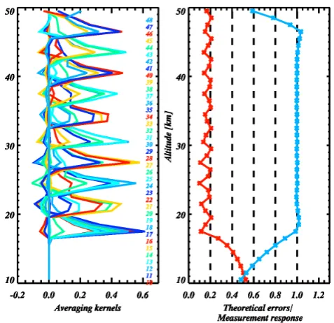
Fig. 11. The left panel shows the averaging kernels and the right
panel shows the theoretical errors (red line) and the measurement re-sponse function (blue line). The measurement is on 13 March 2006, orbit = 21 085, SZA = 109.137 and the moon phase = 0.93.
the averaging kernel matrix A, where A = D K, A≈∂xˆ/∂x. Therefore
A=
KTi S−y1Ki +S−a1
−1
KTi S−y1K. (18) Along with sensitivity of the retrieval, the averaging kernel matrix also characterizes its vertical resolution. At a given altitude, the averaging kernels are peaked functions. The ver-tical resolution is given by their width where a measure of the width at a given height can be FWHM, see Sect. 5.4.4. The sum of all elements (rows) of the averaging kernel ma-trix is often termed the measurement response in the litera-ture (Rodgers, 2000). When it is close to unity, the observing system is sensitive to the true profile. Values less than unity signify the influence of the a priori on the retrieval.
Fig. 12. An example of the retrieved SCIAMACHY lunar
oc-cultation water vapor profile from 10 January 2009, orbit num-ber 35889. For this measurement three collocations are found with ACE-FTS(ss29145), MLS(T505691134), MIPAS(35894).
the retrieval profile is determined only by the measurement (value≈1). Above 47 km there is some contribution from the a priori (value<1).
7 Water vapor profiles
Figure 12 gives an example of the retrieved SCIAMACHY lunar occultation water vapor number density profile for the southern polar stratosphere from 17–50 km. The profile is for 10 January 2009. The correlative ACE-FTS (Atmo-spheric Chemistry Experiment Fourier Transform Spectrom-eter), MLS (Microwave Limb Sounder) and MIPAS (Michel-son Interferometer for Passive Atmospheric Sounding) are also plotted in the figure. The water vapor volume mixing ratios (vmr) from these four instruments were converted to number densities using the temperatures and pressures mea-sured by these instruments. The number densities were then interpolated to the retrieval altitude grid of SCIAMACHY measurements for comparison.
8 Comparisons/validations
To assess the quality of the SCIAMACHY lunar occultation water vapor profiles, the validation was performed with col-located measurements from the satellite instruments ACE-FTS and HALOE (Halogen Occultation Experiment), which are occultation instruments, and MLS and MIPAS, which perform measurements in the limb geometry. The SCIA-MACHY water vapor data showed evidence of PSC as early as May. Such PSCs contaminated profiles were filtered out
Fig. 13. SCIAMACHY–ACE comparison statistics for the period
2004–2009 based on 302 collocations with combined ACE-FTS sunrise and sunset events.
on the basis of the temperature thresholds for the production of all types of PSCs. The formation temperature for the type I PSCs, i.e. nitric acid trihydrate (NAT, crystalline), is less than 195 K, and the type II PSCs, i.e. pure ice, can form at temperatures lower than approximately 188 K (von Savigny et al., 2005; Peter, 1997). The ECMWF analysis profiles cor-responding to the SCIAMACHY water vapor profiles were used as the source of temperature information.
For the comparison with SCIAMACHY data, as men-tioned before, the water vapor vmr from the four instru-ments were converted to number densities. The coincidence search was based on the criteria of selecting all the measure-ments within the maximum collocation radius of 1000 km and having a maximum time difference of 12 h between SCIAMACHY overpass and the correlative measurements from the instruments.
The comparisons are plotted showing the following statistics:
– rmd: The relative mean difference between the SCIA-MACHY and other instrument weighted by the average. – rmd std.: The standard deviation of the ensemble of rel-ative mean differences giving an insight into the vari-ability of the individual comparisons.
Fig. 14. SCIAMACHY–HALOE comparison statistics for the
pe-riod 2003–2005 based on 52 collocations with HALOE sunrise events (none was found with the sunset events).
Fig. 15. SCIAMACHY–MLS comparison statistics for the period
2004–2010 based on 1321 collocations.
As clear in Figs. 13, 14, 15 and 16, the standard error of the bias is very small in all cases as the number of coincidences is large. All biases discussed in the following section are sig-nificant with respect to their standard errors.
8.1 ACE-FTS
The Atmospheric Chemistry Experiment Fourier Transform Spectrometer (ACE-FTS) onboard Canadian scientific satel-lite SCISAT has been performing solar occultation mea-surements in the infrared since 2004 (Bernath, 2005). The
Fig. 16. SCIAMACHY–MIPAS comparison statistics for the period
2005–2010 based on 489 collocations.
vertical resolution of the instrument is consistent with that of SCIAMACHY lunar occultation, which is 3–4 km. The wa-ter vapor vmr from ACE-FTS are retrieved from 5 to 90 km (Carleer et al., 2008). For the presented study, ACE-FTS ver-sion 2.2 water vapor product was used. The comparisons of this version of ACE with various ground-based and space-borne instruments have shown that ACE-FTS is biased pos-itive (wet bias) on the order of 3–10 % between 15–70 km, according to Carleer et al. (2008).
With the collocation criteria described above and for the period of 2004–2009, 302 collocations were found for both sunrise and sunset ACE-FTS events. Figure 13 shows the statistics plotted for the altitude range 17–50 km. The SCIAMACHY–ACE rmd are observed to be within−1.5 % from 17 to 22 km, about −5 % for 23–42 km, around −6 to−7 % between 43–47 km, and within −10 % for the al-titude range 48–50 km. Hence, in general the rmd are below −7 %. The rmd std. are within 5 % from 17 to 29 km and in-crease to 7–10 % from 30 to 50 km. The above mentioned wet bias in ACE-FTS water vapor measurements is also seen by SCIAMACHY lunar occultation measurements. From this evidence, it can be concluded that the SCIAMACHY–ACE agreement is good, being well within the reported biases of ACE-FTS.
8.2 HALOE
The version 19 of HALOE water vapor profiles was used in our study. The extensive validations of HALOE water vapor measurements have shown that HALOE is biased low (dry bias) by 5 % in the stratosphere (Harries et al., 1996; Kley et al., 2000).
The coincidence search with the criteria employed for the years 2003–2005 resulted in 52 coincidences with HALOE sunrise events and none with sunset. Figure 14 shows the statistics of SCIAMACHY–HALOE comparisons. The rmd are 10 % at 17 km, 6 % at 18 km, about 1 % between 19– 24 km, vary around 5 % from 25 to 40 km, within 7.5 % for 41–43 km and reach about 10 % at 50 km. The rmd std. vary between 3.5–4.5 % from 17 to 33 km, 5–6 % at 34–42 km, around 7.5 % for the altitudes 43–48 km and then 10 % to 50 km. Keeping the dry bias in the HALOE measurements in view, the SCIAMACHY–HALOE difference is indicative of the influence of the HALOE bias in the comparisons.
8.3 MLS
The EOS-MLS (Earth Observing System-Microwave Limb Sounder) was launched on NASA’s satellite EOS-Aura in 2004. MLS makes atmospheric measurements from 8 to 90 km by observing thermal microwave emissions from the Earth’s limb (Waters et al., 2006; Schoeberl et al., 2006). In the altitude region of about 18–54 km (100–1.0 hPa), the ver-tical resolution of MLS is 3.5–4.6 km. MLS water vapour version 2.2 was used for the validation of lunar occultation water vapour profiles because it is an extensively validated MLS water vapor product. For the comparison, the MLS geopotential height was converted to geometric height using the MLS pressure and temperature.
The SCIAMACHY–MLS validation was based on 1321 collocated measurements for the period 2004–2010. The comparison result is shown in Fig. 15 where the rmd vary be-tween 1.5–4 % from 17–34 km with exceptions at about 22, 24 and 27 km where it is in the range of±4.5–6 %. The rmd are within−1 to −1.5 % for 35–46 km, and within −3 % from 47 to 50 km. The rmd std. range between 6–7.5 % for the whole altitude of 17–50 km. It should be noted here that in its comparisons with other satellite instruments includ-ing ACE-FTS, HALOE and MIPAS, the MLS water vapor version 2.2 is noted (Lambert et al., 2007) to exhibit sharp differences or kinks around 26.1–31.6 hPa, which is the re-gion within a few kilometres from 25 km. This problem is corrected in the MLS version 3.3 processing algorithm. The SCIAMACHY–MLS exceptional agreement, apart from the above mentioned difference arising due to MLS, validates the good quality of our retrieval and the lunar occultation water vapor dataset. Moreover, MLS, measuring in the mi-crowave, is far less sensitive to clouds and aerosols (Livesey et al., 2006; Waters et al., 2006) that may contaminate any other shorter wavelength region. The SCIAMACHY–MLS excellent agreement shows that the lunar occultation water
vapor measurements used for the validations are void of any contaminations.
8.4 MIPAS
MIPAS (Michelson Interferometer for Passive Atmospheric Sounding) is one of the ten instruments including SCIA-MACHY onboard Envisat satellite. The instrument is a mid-infrared limb emission Fourier transform spectrometer mea-suring atmospheric profiles of temperature and various con-stituents of atmosphere from 6–68 km (Fischer et al., 2008). The vertical resolution of MIPAS varies from around 2.3 km (at 20 km) to about 6.9 km (at 50 km) (von Clarmann et al., 2009). The water vapor data version V40 H2O 203 retrieved from the IMK-IAA data processor was used in the presented comparison. The comparison of this MIPAS water vapor data is performed with various ground-based and satellite instru-ments in the framework of the MOHAVE-2009 campaign, which took place at a location of 34.4◦N, 117◦W on 12–
26 October 2009. The details and results of this study are reported in Stiller et al. (2012). It must be noted that the aim of this campaign was to compare the MIPAS data primarily with highly accurate and precise ground-based and balloon-borne measurements. The MIPAS water vapor profiles are reported to be within±10 % of the profiles of the correlative measurements of most of the instruments, which is within the bias regime among ground-based instruments comparisons.
With the collocation criteria as employed in our study, and for the period of 2005–2010, 489 correlative incidences were found between SCIAMACHY and MIPAS. Figure 16 shows the SCIAMACHY–MIPAS comparison results. The rmd are within−1 to −4.5 % from 17 to 22 km, around−7.5 % at 23–26 km, reach−9 % for the altitude range 27 km to about 38 km, −2.5 to −4.5 % between 39 to 44 km and within −1.5 % for 45–50 km. The rmd std. are about 7.5 % and gradually reach 10 % at 50 km. The SCIAMACHY–MIPAS agreement is within the above mentioned MIPAS bias.
9 Conclusions and outlook
For the southern hemispheric stratosphere, the in situ wa-ter vapor measurements are still in their initial stages and are not available for validation purposes. The SCIAMACHY lu-nar occultation water vapor dataset is valuable for the south-ern hemispheric stratospheric region. The product can be used in the models investigating polar vortex dynamics. With these measurements, the formation of PSCs can be studied as early as May–June for the southern region. The dataset is expected to give good results in interpretations and analyses studies. The lunar occultation water vapor measurements will add as a southern hemispheric coverage to the SCIAMACHY long-term global water vapor time series.
Acknowledgements. We are thankful to the following: ESA EN-VISAT for providing the SCIAMACHY level 1 data. The Atmospheric Chemistry Experiment (ACE) also known as SCISAT, a Canadian-led mission mainly supported by the Canadian SPACE agency and Natural Sciences and Engineering Research Council of Canada. The EOS-MLS (NASA’s mission EOS-AURA). The MIPAS team at Karlsruhe Institute of Technology for providing the data and the updates. The study is funded by the BMBF, DLR-Bonn via grant 50EE0727 and by the University of Bremen.
Edited by: A. J. M. Piters
References
Abbas, M. M., Gunson, M. R., Newchurch, M. J., Michelsen, H. A., Salawitch, R. J., Allen, M. L., Abrams, M. C., Chang, A. Y., Goldman, A., Irion, F. W., Moyer, E. J., Nagaraju, R., Rinsland, C. P., Stiller, G. P., and Zander, R.: The hydro-gen budget of the stratosphere inferred from ATMOS measure-ments of H2O and CH4, Geophys. Res. Lett., 23, 2405–2408, doi:10.1029/96GL01320, 1996.
Amekudzi, L., Bracher, A., Meyer, J., Rozanov, A., Bovensmann, H., and Burrows, J. P.: Lunar occultation with SCIAMACHY, First retrieval results, Adv. Space Res., 5, 906–914, 2005. Amekudzi, L. K.: Stratospheric O3, NO2, and NO3number
den-sity profiles from SCIAMACHY lunar occultation spectro-scopic measurements: Retrieval, validation and interpretation, Ph.D. thesis, Universit¨at Bremen, 2005.
Amekudzi, L. K., Bramstedt, K., Rozanov, A., Bovensmann, H., and Burrows, J. P.: Retrievals of trace gas concentratioins from lu-nar occultation measurements with SCIAMACHY on ENVISAT, in: New Horizon in occultation Research: Studies in Atmosphere and Climate, Springer, Berlin, Heidelberg, 87–96, 2009.
of atmospheric constituents from moderate resolution radiance measurements in the visible/near-infrared spectral region, J. Geophys. Res., 105, 15247–15261, doi:10.1029/2000JD900171, 2000.
Burrows, J. P., Holzle, E., Goede, A. P. H., Visser, H., and Fricke, W.: SCIAMACHY – Scanning Imaging Absorption Spectrome-ter for Atmospheric Chartography, Acta Astronaut., 35, 445–451, 1995.
Carleer, M. R., Boone, C. D., Walker, K. A., Bernath, P. F., Strong, K., Sica, R. J., Randall, C. E., V¨omel, H., Kar, J., H¨opfner, M., Milz, M., von Clarmann, T., Kivi, R., Valverde-Canossa, J., Sioris, C. E., Izawa, M. R. M., Dupuy, E., McElroy, C. T., Drummond, J. R., Nowlan, C. R., Zou, J., Nichitiu, F., Los-sow, S., Urban, J., Murtagh, D., and Dufour, D. G.: Validation of water vapour profiles from the Atmospheric Chemistry Ex-periment (ACE), Atmos. Chem. Phys. Discuss., 8, 4499–4559, doi:10.5194/acpd-8-4499-2008, 2008.
Dessler, A. and Kim, H.: Determination of the amount of water va-por entering the stratosphere based on Halogen Occultation Ex-periment (HALOE) data, J. Geophys. Res., 104, 30605–30607, 1999).
Fischer, H., Birk, M., Blom, C., Carli, B., Carlotti, M., von Clar-mann, T., Delbouille, L., Dudhia, A., Ehhalt, D., EndeClar-mann, M., Flaud, J. M., Gessner, R., Kleinert, A., Koopman, R., Langen, J., L´opez-Puertas, M., Mosner, P., Nett, H., Oelhaf, H., Perron, G., Remedios, J., Ridolfi, M., Stiller, G., and Zander, R.: MIPAS: an instrument for atmospheric and climate research, Atmos. Chem. Phys., 8, 2151–2188, doi:10.5194/acp-8-2151-2008, 2008. Fu, Q. and Liou, K. N.: On the correlated k-distribution method
for radiative transfer in nonhomogeneous atmospheres, J. Atmos. Sci., 49, 2139–2156, 1992.
Gottwald, M. and Bovensmann, H. (Eds.): Exploring the Changing Earth’s Atmosphere, Springer, Dordrecht, Heidelberg, London, New York, doi:10.1007/978-90-481-9896-2, 2011.
Gurlit, W., Zimmermann, R., Giesemann, C., Fernholz, T., Ebert, V., Wolfrum, J., Platt, U., and Burrows, J. P.: Lightweight diode laser spectrometer CHILD (Compact High-altitude In-situ Laser Diode) for balloonborne measurements of water vapor and methane, Appl. Optics, 44, 91–102, 2005.
Harries, J. E., Russell, J. M. I., Tuck, A. F., Gordley, L. L., Pur-cell, P., Stone, K., Bevilacqua, R. M., Nedoluha, G., and Traub, W. A.: Validation of measurements of water vapor from the Halo-gen Occultation Experiment (HALOE), J. Geophys. Res., 101, 10205–10216, doi:10.1029/95JD02933, 1996.
Kirk-Davidoff, D. B. and Lamarque, J.-F.: Maintenance of polar stratospheric clouds in a moist stratosphere, Clim. Past, 4, 69– 78, doi:10.5194/cp-4-69-2008, 2008.
Kirk-Davidoff, D. B., Hintsa, E. J., Anderson, J. G., and Keith, D. W.: The effect of climate change on ozone depletion through changes in stratospheric water vapour, Nature, 402, 399–401, 1999.
Kley, D., Russell III, J. M., and Phillips, C. (Eds.): SPARC assess-ment upper tropospheric and stratospheric water vapour, WCRP-No. 113, WMO/TD-WCRP-No. 1043, SPARC Report WCRP-No. 2, WCRP, Geneva, Switzerland, 2000.
Kratz, D. P., Chou, M.-D., Yan, M. M.-H., and Ho, C.-H.: Mi-nor trace gas radiative forcing calculations using the k distribu-tion method with one-parameter scaling, J. Geophys. Res., 103, 31647–31656, doi:10.1029/1998JD200009, 1998.
Lahoz, W. A., Carr, E. S., Froidevaux, L., Harwood, R. S., Kumer, J. B., Mergenthaler, J. L., Peckham, G. E., Read, W. G., Ri-caud, P. D., Roche, A. E., and Waters, J. W.: Northern hemi-sphere mid – stratohemi-sphere vortex processes diagnosed from H2O, N2O, and potential vorticity, Geophys. Res. Lett., 20, 2671– 2674, doi:10.1029/93GL02475, 1993.
Lahoz, W. A., O’Neill, A., Heaps, A., Pope, V. D., Swinbank, R., Harwood, R. S., Froidevaux, L., Read, W. G., Waters, J. W., and Peckham, G. E.: Vortex dynamics and the evolution of water vapour in the stratosphere of the southern hemisphere, Q. J. Roy. Meteorol. Soc., 122, 423–450, doi:10.1002/qj.49712253007, 1996.
Lambert, A., Read, W. G., Livesey, N. J., Santee, M. L., Manney, G. L., Froidevaux, L., Wu, D. L., Schwartz, M. J., Pumphrey, H. C., Jimenez, C., Nedoluha, G. E., Cofield, R. E., Cuddy, D. T., Daffer, W. H., Drouin, B. J., Fuller, R. A., Jarnot, R. F., Knosp, B. W., Pickett, H. M., Perun, V. S., Snyder, W. V., Stek, P. C., Thurstans, R. P., Wagner, P. A., Waters, J. W., Jucks, K. W., Toon, G. C., Stachnik, R. A., Bernath, P. F., Boone, C. D., Walker, K. A., Urban, J., and Murtagh, D.: Validation of the Aura Mi-crowave Limb Sounder middle atmosphere water vapor and ni-trous oxide measurements, J. Geophys. Res., 112, 1–24, 2007. Li, J. and Barker, H. W.: A Radiation Algorithm with
Correlated-k Distribution, Part I: Local Thermal Equilibrium, Physics, 62, 286–309, doi:10.1175/JAS-3396.1, 2004.
Livesey, N. J., Synder, W. V., Read, W. G., and Wagner, P. A.: Retrieval algorithms for the EOS 10 Microwave Limb Sounder (MLS), IEEE T. Geosci. Remote, 44, 1144–1155, 2006. Michelsen, H. A., Irion, F. W., Manney, G. L., Toon, G. C., and
Gun-son, M. R.: Features and trends in Atmospheric Trace Molecule Spectroscopy (ATMOS) version 3 stratospheric water vapor and methane measurements, J. Geophys. Res., 105, 22713–22724, doi:10.1029/2000JD900336,2000.
NASA: US Standard Atmosphere Supplements, US Government Printing Office, Washington, D.C., 1976.
Pan, L. L., Randel, W. J., Massie, S. T., Kanzawa, H., Sasano, Y., Nakajima, H., Yokota, T., and Sugita, T.: Variability of polar stratospheric water vapor observed by ILAS, J. Geophys. Res., 107, 8214, doi:10.1029/2001JD001164, 2002.
Pan, L. L., Bowman, K. P., Shapiro, M., Randel, W. J., Gao, R. S., Campos, T., Davis, C., Schauffler, S., Ridley, B. A., Wei, J. C., and Barnet, C.: Chemical behavior of the tropopause observed during the Stratosphere-Troposphere Analyses of Regional Transport experiment, J. Geophys. Res., 112–124,
doi:10.1029/2007JD008645, 2007.
Peter, T.: Microphysics and heterogeneous chemistry of polar stratospheric clouds, Annu. Rev. Phys. Chem., 48, 785–822, 1997.
Rodgers, C. D.: Inverse Methods for Atmospheric Sounding: The-ory and Practice, World Scientific, Singapore, 2000.
Rothman, L., Gordon, I., Barbe, A., Benner, D. C., Bernath, P., Birk, M., Brown, L., Campargue, A., Champion, J.-P., Chance, K., Coudert, L., Dana, V., Devi, V., Fally, S., Flaud, J.-M., Gamache, R., Goldman, A., Jacquemart, D., Kleiner, I., Lacome, N., Laf-ferty, W., Mandin, J., Massie, S., Mikhailenko, S., Miller, C., Moazzen-Ahmadi, N., Naumenko, O., Nikitin, A., Orphal, J., Perevalov, V., Perrin, A., Predoi-Cross, A., Rinsland, C., Rot-ger, M., Simeckova, M., Smith, M., Sung, K., Tashkun, S., Ten-nyson, J., Toth, R., Vandaele, A., and Vander Auwera, J.: The HI-TRAN 2008 molecular spectroscopic database, J. Quant. Spectr. Ra., 110, 533–572, doi:10.1016/j.jqsrt.2009.02.013, 2009. Rozanov, A.: Modelling of the radiative transfer through a
spher-ical planetary atmosphere: application to the atmospheric trace gas retrieval from occultation and limb measurements in UV-Vis-NIR, Ph.D. thesis, Universit¨at Bremen, 2001.
Rozanov, A., Rozanov, V., Buchwitz, M., Kokhanovsky, A., and Burrows, J. P.: SCIATRAN 2.0 – A new radiative transfer model for geophysical applications in the 175–2400 nm spec-tral region, Adv. Space Res., 36, 1015–1019, doi:10.1016/S0273-1177(02)00095-9, 2005.
Rozanov, A., Weigel, K., Bovensmann, H., Dhomse, S., Eichmann, K.-U., Kivi, R., Rozanov, V., V¨omel, H., Weber, M., and Bur-rows, J. P.: Retrieval of water vapor vertical distributions in the upper troposphere and the lower stratosphere from SCIA-MACHY limb measurements, Atmos. Meas. Tech., 4, 933–954, doi:10.5194/amt-4-933-2011, 2011.
Rozanov, A. V., Rozanov, V. V., and Burrows, P. J.: Combined differential-integral approach for the radiation field computation in a spherical shell atmosphere: Nonlimb geometry, J. Geophys. Res., 105, 22937–22942, doi:10.1029/2000JD900378, 2000. Rozanov, V. V., Diebel, D., Spurr, R. J. D., and Burrows, J. P.:
GOMETRAN: A radiative transfer model for the satellite project GOME, the plane-parallel version, J. Geophys. Res., 102, 16683–16695, doi:10.1029/96JD01535, 1997.
Russell, J. M. I., Tuck, A. F., Gordley, L. L., Park, J. H., Drayson, S. R., Harries, J. E., Cicerone, R. J., and Crutzen, P. J.: HALOE Antarctic observations in the spring of 1991, Geophys. Res. Lett., 20, 719–722, doi:10.1029/93GL00497, 1993a.
Russell, J. M. I., Gordley, L. L., Park, J. H., Drayson, S. R., Hesketh, W. D., Cicerone, R. J., Tuck, A. F., Frederick, J. E., Harries, J. E., and Crutzen, P. J.: The Halogen Occultation Experiment, J. Geo-phys. Res., 98, 10777–10797, doi:10.1029/93JD00799, 1993b. Schoeberl, M., Douglass, A., Hilsenrath, E., Bhartia, P., Beer,
R., Waters, J., Gunson, M., Froidevaux, L., Gille, J., Bar-nett, J., Levelt, P., and DeCola, P.: Overview of the EOS aura mission, Geosci. Remote Sens., 44, 1066–1074, doi:10.1109/TGRS.2005.861950, 2006.
a method of regularization, 151, Dokl. Acad. Nauk, SSSR, 501– 504,, 1963.
Tikhonov, A. N. and Arsenin, V. Y.: Solutions of ill-Posed Prob-lems, Wiley, New York, 1977.
von Clarmann, T., H¨opfner, M., Kellmann, S., Linden, A., Chauhan, S., Funke, B., Grabowski, U., Glatthor, N., Kiefer, M., Schiefer-decker, T., Stiller, G. P., and Versick, S.: Retrieval of temperature, H2O, O3, HNO3, CH4, N2O, ClONO2and ClO from MIPAS reduced resolution nominal mode limb emission measurements, Atmos. Meas. Tech., 2, 159–175, doi:10.5194/amt-2-159-2009, 2009.
Chen, G. S., Chudasama, M. V., Dodge, R., Fuller, R. A., Gi-rard, M. A., Jiang, J. J., Jiang, Y., Knosp, B. W., LaBelle, R. C., Lam, J. C., Lee, K. A., Miller, D., Oswlad, J. E., Patel, N. C., Pukala, D. M., Quintero, O., Scaff, D. M., Van Synder, W., Tope, M. C., Wagner, P. A., and Walch, M. J.: The Earth Observing Sys-tem Microwave Limb Sounder (EOS MLS) on the Aura satellite, IEEE T. Geosci. Remote, 44, 1075–1092, 2006.