www.the-cryosphere.net/9/465/2015/ doi:10.5194/tc-9-465-2015
© Author(s) 2015. CC Attribution 3.0 License.
Geophysical mapping of palsa peatland permafrost
Y. Sjöberg1, P. Marklund2, R. Pettersson2, and S. W. Lyon1
1Department of Physical Geography and the Bolin Centre for Climate Research, Stockholm University, Stockholm, Sweden 2Department of Earth Sciences, Uppsala University, Uppsala, Sweden
Correspondence to: Y. Sjöberg (ylva.sjoberg@natgeo.su.se)
Received: 15 August 2014 – Published in The Cryosphere Discuss.: 13 October 2014 Revised: 3 February 2015 – Accepted: 10 February 2015 – Published: 4 March 2015
Abstract. Permafrost peatlands are hydrological and bio-geochemical hotspots in the discontinuous permafrost zone. Non-intrusive geophysical methods offer a possibility to map current permafrost spatial distributions in these envi-ronments. In this study, we estimate the depths to the per-mafrost table and base across a peatland in northern Swe-den, using ground penetrating radar and electrical resistivity tomography. Seasonal thaw frost tables (at ∼0.5 m depth), taliks (2.1–6.7 m deep), and the permafrost base (at ∼16 m depth) could be detected. Higher occurrences of taliks were discovered at locations with a lower relative height of per-mafrost landforms, which is indicative of lower ground ice content at these locations. These results highlight the added value of combining geophysical techniques for assessing spa-tial distributions of permafrost within the rapidly changing sporadic permafrost zone. For example, based on a back-of-the-envelope calculation for the site considered here, we es-timated that the permafrost could thaw completely within the next 3 centuries. Thus there is a clear need to benchmark cur-rent permafrost distributions and characteristics, particularly in under studied regions of the pan-Arctic.
1 Introduction
Permafrost peatlands are widespread across the Arctic and cover approximately 12 % of the arctic permafrost zone (Hugelius et al., 2013; Hugelius et al., 2014). They often occur in sporadic permafrost areas, protected by the peat cover, which insulates the ground from heat during the sum-mer (Woo, 2012). In the sporadic permafrost zone, the per-mafrost ground temperature is often close to 0◦C, and there-fore even small increases in temperature can result in thawing of permafrost. In addition, permafrost distribution and
thaw-ing in these landscapes are influenced by several factors other than climate, including hydrological, geological, morpholog-ical, and erosional processes that often combine in complex interactions (e.g., McKenzie and Voss, 2013; Painter et al., 2013; Zuidhoff, 2002). Due to these interactions, peatlands are often dynamic with regards to their thermal structures and extent, as the distribution of permafrost landforms (such as dome-shaped palsas and flat-topped peat plateaus) and talik landforms (such as hollows, fens, and lakes) vary with cli-matic and local conditions (e.g., Sannel and Kuhry, 2011; Seppälä, 2011; Wramner, 1968). This dynamic nature and variable spatial extent has potential implications across the pan-Arctic as these permafrost peatlands store large amounts of soil organic carbon (Hugelius et al., 2014; Tarnocai et al., 2009). The combination of large carbon storage and high po-tential for thawing make permafrost peatlands biogeochem-ical hotspots in the warming Arctic. In light of this, predic-tions of future changes in these environments require knowl-edge of current permafrost distributions and characteristics, which is sparse in today’s scientific literature.
peat-lands make up a large portion of the peat-landscape mosaic and regional-scale differences exist in carbon fluxes (Giesler et al., 2014).
Geophysical methods offer non-intrusive techniques for measuring physical properties of geological materials; how-ever, useful interpretation of geophysical data requires other types of complementary data, such as sediment cores. Ground penetrating radar (GPR) has been used extensively in permafrost studies for identifying the boundaries of per-mafrost (e.g., Arcone et al., 1998; Doolittle et al., 1992; Hinkel et al., 2001; Moorman et al., 2003), characterizing ground ice structures (De Pascale et al., 2008; Hinkel et al., 2001; Moorman et al., 2003), and estimating seasonal thaw depth and moisture content of the active layer (Gacitua et al., 2012; Westermann et al., 2010). Electrical resistivity tomog-raphy (ERT) has also been widely applied in permafrost stud-ies (Hauck et al., 2003; Ishikawa et al., 2001; Kneisel et al., 2000), the majority of which focus on mountain permafrost. By combining two or more geophysical methods comple-mentary information can often be acquired raising the con-fidence in interpretations of permafrost characteristics (De Pascale et al., 2008; Hauck et al., 2004; Schwamborn et al., 2002). For example, De Pascale et al. (2008) used GPR and capacitive-coupled resistivity to map ground ice in continu-ous permafrost and demonstrated the added value of combin-ing radar and electrical resistivity measurements for the qual-ity of interpretation of the data. While some non-intrusive geophysical investigations have been done in palsa peatland regions (Dobinski, 2010; Doolittle et al., 1992; Kneisel et al., 2007, 2014; Lewkowicz et al., 2011), the use of multiple geo-physical techniques to characterize the extent of permafrost in palsa peatland environments has not been employed.
In this study we use GPR and ERT in concert to map the distribution of permafrost along three transects (160 to 320 m long) in the Tavvavuoma palsa peatland in northern Sweden. Our aim is to understand how depths of the permafrost table and base vary in the landscape and, based on resulting esti-mates of permafrost thickness, to make a first-order assess-ment of the potential time needed to completely thaw this permafrost due to climate warming. Furthermore, we hope to demonstrate the added value of employing complemen-tary geophysical techniques in such landscapes. This novel investigation thus helps contribute to our understanding of the current permafrost distribution and characteristics across palsa peatlands, creating a baseline for future studies of pos-sible coupled changes in hydrology and permafrost distribu-tion in such areas.
2 Study area
Tavvavuoma is a large palsa peatland complex in northern Sweden at 68◦280N, 20◦540E, 550 m a.s.l. (Fig. 1) and con-sists of a patchwork of palsas, peat plateaus, thermokarst lakes, hummocks, and fens. Ground temperatures and
! ! ! ! ! ! ! ! ! ! ! ! ! ! ! ! ! ! ! ! ! ! ! ! ! ! ! !!!!!!!!!!!!!!!!!!!!!!!!!!!!!!!!!!!!!!!!!!!!!!!!!!!!!!!!!!!!!!!!!!!!!!!!!!!!!!!!!!!!!!!!!!!!!!!!!!!!!!!!!!!!!!!!!!!!!!!!!!!!!!!!!!!!!!!!!!!!!!!!!!!!!!!!!!!!!!!!!!!!!!!!!!!!!!!!!!!!!!!!!!!!!!!!!!!!!!!!!!!!!!!!!!!!!!!!!!!!!!!!!!!!!!!!!!!!!!!!!!!!!!!!!!!!!!!!!!!!!!!!!!!!!!!!!!!!!!!!!!!!!!!!!!!!!!!!!!!!!!!!!!!!!!!!!!!!!!!!!!!!!!!!!!!!!!!!!!!!!!!!!!!!!!!!!!!!!!!!!!!!!!!!!!!!!!!!!!!!!!!!!!!!!!!!!!!!!!!!!!!!!!!!!!!!!!!!!!!!!!!!!!!!!!!!!!!!!!!!!!!!!!!!!!!!!!!!!!!!!!!!!!!!!!!!!!!!!!!!!!!!!!!!!!!!!!!!!!!!!!!!!!!!!!!!!!!!!!!!!!!!!!!!!!!!!!!!!!!!!!!!!!!!!!!!!!!!!!!!!!!!!!!!!!!!!!!!!!!!!!!!!!!!!!!!!!!!!!!!!!!!!!!!!!!!!!!!!!!!!!!!!!!!!!!!!!!!!!!!!!!!!!!!!!!!!!!!!!!!!!!!!!!!!!!!!!!!!!!!!!!!!!!!!!!!!!!!!!!!!!!!!!!!!!!!!!!!!!!!!!!!!!!!!!!!!!!!!!!!!!!!!!!!!!!!!!!!!!!!!!!!!!!!!!!!!!!!!!!!!!!!!!!!!!!!!!!!!!!!!!!!!!!!!!!!!!!!!!!!!!!!!!!!!!!!!!!!!!!!!!!!!!!!!!!!!!!!!!!!!!!!!!!!!!!!!!!!!!!!!!!!!!!!!!!!!!!!!!!!!!!!!!!!!!!!!!!!!!!!!!!!!!!!!!!!!!!!!!!!!!!!!!!!!!!!!!!!!!!!!!!!!!!!!!!!!!!!!!!!!!!!!!!!!!!!!!!!!!!!!!!!!!!!!!!!!!!!!!!!!!!!!!!!!!!!!!!!!!!!!!!!!!!!!!!!!!!!!!!!!!!!!!!!!!!!!!!!!!!!!!!!!!!!!!!!!!!!!!!!!!!!!!!!!!!!!!!!!!!!!!!!!!!!!!!!!!!!!!!!!!!!!!!!!!!!!!!!!!!!!!!!!!!!!!!!!!!!!!!!!!!!!!!!!!!!!!!!!!!!!!!!!!!!!!!!!!!!!!!!!!!!!!!!!!!!!!!!!!!!!!!!!!!!!!!!!!!!!!!!!!!!!!!!!!!!!!!!!!!!!!!!!!!!!!!!!!!!!!!!!!!!!!!!!!!!!!!!!!!!!!!!!
0 50 100 Meters
T1 T2 1 5 4 3 2 7 T3 6 40°0'0"E 10°0'0"W 20°0'0"E 7 0 °0 '0 "N 6 0 °0 '0 "N
0 50 100 Meters
T1 T2 1 5 4 3 2 6 7 T3 1 2 3 4 5 6 Investigated transects
10 m borehole 6 m borehole 2 points of 2 m coring 2 m coring point 2 points of 2 m coring CMP profile (saturated peat) Direction of transects
N 7
0 °0’ 0”N 60 °0’ 0”N
Figure 1. Location of the study site (inset), investigated transects,
existing boreholes (Ivanova et al., 2011, points 1 and 2), coring points, and point of CMP measurement (described in Sect. 3.1; aerial photograph from Lantmäteriet, the Swedish land survey, 2012).
weather parameters have been monitored at the site since 2005 (Christiansen et al., 2010). Sannel and Kuhry (2011) have analyzed lake changes in the area and detailed local studies of palsa morphology have been conducted by Wram-ner (1968, 1973).
Tavvavuoma is located on a flat valley bottom, in piedmont terrain with relative elevations of surrounding mountains about 50 to 150 m above the valley bottom. Unconsolidated sediments, observed from two borehole cores (points 1 and 2 in Fig. 1), are of mainly glaciofluvial and lacustrine origin and composed of mostly sands, loams, and coarser-grained rounded gravel and pebbles (Ivanova et al., 2011). The mean annual air temperature is−3.5◦C (Sannel and Kuhry, 2011), and the average winter snow cover in Karesuando, a mete-orological station approximately 60 km east of Tavvavuoma, is approximately 50 cm, although wind drift generally gives a thinner snow cover in Tavvavuoma (Swedish Meteorological and Hydrological Institute, http://www.smhi.se/klimatdata/ meteorologi).
Permafrost occurs primarily under palsas and peat plateaus in Tavvavuoma, where the average thickness of the active layer is typically 0.5 m (Christiansen et al., 2010; Sannel and Kuhry, 2011). The mean annual temperature in permafrost boreholes is 2◦C (Christiansen et al., 2010). However, no
in Abisko (located about 60 km southwest of Tavvavuoma) is increasing according to direct observation over the past 30 years (Åkerman and Johansson, 2008) and inference from hydrologic shifts over the past century (Lyon et al., 2009). This regional permafrost degradation has led to changes in palsas as well. Regionally, reductions in both areas covered by palsas and palsa height have been observed (Sollid and Sorbel, 1998; Zuidhoff, 2002; Zuidhoff and Kolstrup, 2000). In Tavvavuoma, both growth and degradation of palsas have been observed in detailed morphological studies during the 1960s and 1970s (Wramner, 1968, 1973), and expansion and infilling of thermokarstic lakes have been observed through remote sensing analyses (Sannel and Kuhry, 2011). Palsa degradation and infilling of lakes with fen vegetation have been the dominating processes during recent years (Sannel and Kuhry, 2011; Wramner et al., 2012).
3 Theory and methods
Measurements of permafrost extent and structure were made with both GPR and ERT between 20 and 26 August 2012 along three transects covering the main permafrost landforms in the Tavvavuoma area (Fig. 1). The ERT transects were somewhat extended (i.e., slightly longer) compared to the GPR transects to increase the penetration depth along the overlapping parts of the transects.
Transect T1 was 160 m long and crossed a peat plateau that was raised approximately 1.5 m above the surrounding landscape (Fig. 1). It further crossed two thermokarst de-pressions (centered at 45 and 130 m) within the peat plateau. Transect T2 was 320 m long, but the southern part cover-ing about 180 m could not be measured with GPR due to dense vegetation cover (mainly Salix sp.). Transect T2 started on a peat plateau surface at the edge of a drained lake and continued north over a fen (110–180 m) and a small stream (140 m). The northern part, measured with both ERT and GPR, crossed a palsa (200 m) that was raised about 4 m above the surrounding landscape. This palsa has been described via a borehole profile (Ivanova et al., 2011; point 1 in Fig. 1). Transect T2 then continued across two fens (250 and 290 m) separated by a lower palsa (270 m). Transect T3 was 275 m long. It started on a relatively low palsa and stretched over a flat area covered by hummocks and thermokarst depressions. In addition to the geophysical investigations (details of which are described in the following sections), the depth to the permafrost table (the active layer) was probed every 2 m along all transects using a 1 m steel rod. Sediment cores were retrieved at four points along T1 and two points along T3 down to 2 m. These cores were used to locate the depth to the peat–mineral substrate interface and the depth to the per-mafrost table (at points 3, 4, 5, and 6 in Fig. 1). The topog-raphy was measured along the transects using a differential GPS with supplemental inclinometer observations along pro-files where only ERT was used. The position of the transects
was measured using a tape measure and marked at regular intervals to ensure that locations of GPR and ERT transects coincided.
3.1 Ground penetrating radar
Ground penetrating radar (GPR) can be used to map near surface geology and stratigraphy because of differences in dielectric properties between different subsurface layers or structures. An electromagnetic pulse is transmitted through the ground and the return time of the reflected pulse is recorded. The resolution and penetration depth of the radar signal depends on the characteristics of the transmitted pulse and the choice of antennas, which usually range between 10 and 1000 MHz. Higher frequencies will yield a higher resolution but a smaller penetration depth; however, the pen-etration depth will also depend on dielectric and conductive properties of the ground material. Mapping of permafrost us-ing GPR becomes possible due to the difference in permittiv-ity between unfrozen and frozen water.
In this study, measurements were made with a Malå Geo-Science ProEx GPR system using 200 MHz unshielded tennas along T1 and T2. The transmitting and receiving an-tennas were held at a constant distance of 0.6 m (common offset) and the sampling time window was set to 621 ns, with recorded traces stacked 16 times. Measurements were made at every 10 cm along the length of these two transects. Along T3, measurements were made using 100 MHz unshielded antennas with a 1 m antenna separation and measurements made every 0.2 s while moving the antennas along the tran-sect. The sampling time window for T3 was 797 ns and traces were stacked 16 times. The GPR data were processed for a time-zero correction and with a dewow filter, a vertical gain, and a normal-moveout correction for antenna geometry using the software ReflexW (version 6.1, Sandmeier Geophysical Research, 2012, http://www.sandmeier-geo.de).
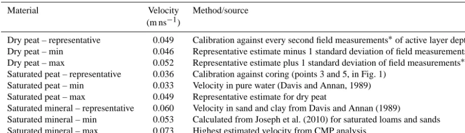
Table 1. Velocities used for converting two-way travel times to depth in GPR data.
Material Velocity Method/source
(m ns−1)
Dry peat – representative 0.049 Calibration against every second field measurements∗of active layer depths Dry peat – min 0.046 Representative estimate minus 1 standard deviation of field measurements∗ Dry peat – max 0.052 Representative estimate plus 1 standard deviation of field measurements∗ Saturated peat – representative 0.036 Calibration against coring (points 3 and 5, in Fig. 1)
Saturated peat – min 0.033 Velocity in pure water (Davis and Annan, 1989) Saturated peat – max 0.049 Representative estimate for dry peat
Saturated mineral – representative 0.060 Velocity in sand and clay from Davis and Annan (1989)
Saturated mineral – min 0.053 Calculated from Joseph et al. (2010) for saturated loams and sands Saturated mineral – max 0.073 Highest estimated velocity from CMP analysis
∗Field measurement using a 1 m steel rod.
0,03 0,05 0,07 0,09 Velocity [m/ns] 0,045 0,05 0,055
De
p
th
Palsa velocity profile
Talik velocity profile
Dry peat
Frozen ground
Saturated peat
Saturated mineral Profile
Profile
De
p
th
Ground surface
Peat–mineral interface
Unfrozen–frozen interface
Velocity [m/ns]
Minimum velocity
Representative velocity
Maximum velocity
Figure 2. Conceptual sketch of typical distribution of ground substrates and associated estimated velocities for a palsa and talik ground
profile.
adding 1 standard deviation of the measured depths, respec-tively. For velocities in saturated peat that was found in taliks such as fens, the thickness of the saturated peat layer identi-fied by coring with a 2 m steel pipe (points 3 and 5, Fig. 1) was used. The velocity in pure water was used as the min-imum velocity and the representative velocity for dry peat was used as the maximum velocity for saturated peat.
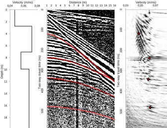
To obtain velocities for unfrozen saturated mineral sub-strate, a common midpoint (CMP) GPR profile was mea-sured on a drained lake surface (point 7 in Fig. 1). Coring down to 2 m with a steel pipe at this location revealed the existence of an unfrozen saturated peat layer down to 1.75 m depth and unfrozen mineral soils consisting of mainly sand and silt below that depth. CMP analysis is a widely used method to estimate local GPR signal velocities through ground materials. By moving GPR transmitting and receiv-ing antennas apart incrementally between measurements, the same point in space is imaged with different antenna off-sets, making it possible to back out material velocity esti-mates from the hyperbolic shape of the recorded reflectors.
0
10
0
20
0
30
0
40
0
50
0
60
0
1 2 3 4 5 6 7 8 9 10 11 12 13 14 15 16
0
10
0
20
0
30
0
40
0
50
0
60
0
0,03 0,05 0,07 0,09 0
2
4
6
8
10
12
14
16
18
20
0,04 0,06 0,08
Velocity (m/ns) Distance (m) Velocity (m/ns)
Dept
h (m
)
T
w
o
-w
ay
tr
av
el
ti
m
e
(ns
)
T
w
o
-w
ay
tr
av
el
ti
m
e
(ns
)
Figure 3. Estimated velocity profile, recorded CMP radargram, and semblance plot for the CMP transect measured on the drained lake
surface. The semblance plot shows more likely velocities in darker shades of grey with the velocities from the reflectors (red lines in radargram) used for generating the velocity profile indicated by black and red diamonds.
in constraining the material velocities for the deeper layers using this method, these results were only used for estimat-ing a probable maximum velocity in unfrozen mineral sedi-ments (as this was higher than most literature values). This maximum velocity estimate was complemented with litera-ture values for the representative and minimum velocities. 3.2 Electrical resistivity tomography
Direct-current electrical resistivity measurements are based on a measured potential difference between two electrodes (1V ) inserted with galvanic coupling to the ground and, similarly, two electrodes where current is injected into the ground (I) with a known geometric factor (k) depending on the arrangement of the electrodes. This gives a value of the apparent resistivity (ρa) of the ground subsurface as
ρa=k1V / l. (1)
During a tomographic resistivity survey, many of these mea-surements are made in lateral and vertical directions (by in-creasing the electrode spacing). The acquired data are subse-quently modeled to generate an image of the resistivity distri-bution under the site. Values of resistivity vary substantially with grain size, porosity, water content, ice content, salin-ity, and temperature (e.g., Reynolds, 2011); thus, the resis-tivity of permafrost also varies to a large degree. This makes
ERT techniques useful in detecting the sharp contrast be-tween frozen and unfrozen water content within sediments.
At the Tavvavuoma site, measurements of electrical resis-tivity were made with the Terrameter LS from ABEM and an electrode spacing of 2 m for the T1 transect and 4 m for the T2 and T3 transects. The Wenner array configuration for the electrodes was used due to its high signal-to-noise ratio and for its accuracy in detecting vertical changes over other common array types (Loke, 2010). For the inverse model-ing, the smoothness-constrained least-square method was ap-plied (Loke and Barker, 1996). The inversion progress was set to stop when the change in root mean squared error from the previous iteration was less than 5 % (implying conver-gence of the inversion). The software Res2dinv (v.3.59.64, Geotomo Software, Loke, 2010) was used for the inverse modeling during this study.
dif-ference scheme where 0.1 and 10 times the average apparent resistivity of the resistivity model was considered (respec-tively) for the initial reference resistivity parameter. Normal-ized DOI values higher than 0.1 indicate that the model is likely not constrained by the data and should be given little significance in subsequent model interpretation.
To further validate the ERT interpretations, one shorter transect with 0.5 m electrode spacing was conducted over a palsa. This was used to acquire a local resistivity value for the interface between unfrozen and frozen sediments at the bot-tom of the active layer. This value (1700m) allowed us to map permafrost boundaries in the ERT images, with all resis-tivity values>1700m interpreted as permafrost. However, as the resistivity of the ground varies with other sediment physical properties and the sediment distribution is complex at the site, the resistivity boundary value for permafrost will naturally vary along transects and with depth. For instance, sands generally have maximum values for the unfrozen state close to 1200m and for some gravels this can reach up to 3000m (Hoekstra et al., 1974). Finer sediments, such as clays and silts, have lower values ranging from ca. 80 to 300m (Hoekstra et al., 1974). At our site sands dominate, but there is also evidence of loams. Lewkowicz et al. (2011) report a resistivity of 1000m at the base of permafrost un-der a palsa in similar, but somewhat finer, sediment con-ditions in southern Yukon. This value from Lewkowicz et al. (2011) was thus used as a possible minimum resistiv-ity value for the permafrost boundary in the interpretations, while the local resistivity estimate (1700m) was used as a maximum and representative value. All resistivity val-ues<1000m were thus interpreted as unfrozen ground and the values between 1000 and 1700m represent a range of uncertainty for the location of the interface between frozen and unfrozen sediments. Again, the motivation here was to account for potential uncertainty allowing for robust inter-pretation.
3.3 Calculations of active layer thickness and future thaw rates
To help put the geophysical measurements and their poten-tial implications for this peatland palsa region in context, the thickness of the active layer as well as first-order estimate of long-term thaw rates were estimated using a simple equa-tion for 1-D heat flow by conducequa-tion, the Stefan equaequa-tion (as described by Riseborough et al., 2008):
Z= r
2λI
Ln, (2)
where Z is the thaw depth,λ is thermal conductivity,I is the thawing degree day index (as described by Nelson and Outcalt, 1987),Lis the volumetric latent heat of fusion, and nis the saturated porosity of the ground substrate. As a talik is by definition unfrozen ground occurring in a permafrost area, Eq. (2) was used to confirm that ground identified as
talik in Tavvavuoma through the GPR and ERT images did not correspond to locations of deeper active layer relative to surrounding positions (i.e., provide a confirmation that these sites would not freeze during winter).
Calculations of active layer depths in fens were made using a sinusoidal annual air temperature curve generated from the average temperature of the warmest and the cold-est months of the year as input. The effect of the snow cover, which would give higher ground-surface temperatures in the winter, was not explicitly taken into consideration in this sim-ple calculation as we did not have any direct estimates of snow cover available for the transects. As such, these calcula-tions are simply a first-order approximation. Representative properties for saturated peat (the most common material in the uppermost part of the ground in suspected taliks) were chosen, including a thermal conductivity of 0.5 W m−1K−1
and a saturated fraction of 0.80 (Woo, 2012).
In addition, a first-order approximation of long-term thaw rates was carried out. An instantaneous increase in air tem-perature of 2◦C was assumed, which represents a warming within current climate projections for the 21st century, al-though at the low end of projections for Arctic warming (IPCC, 2013). Material properties for this calculation were based on information on deeper sediment layers from the 10 m borehole (Ivanova et al. 2011, point 1 in Fig. 1). A sat-urated fraction of 0.5, representative of sand slightly over-saturated with ice, was used. To account for some of the uncertainty in this rough estimate, a range of likely mini-mum and maximini-mum values for thermal conductivity (2 and 3 W m−1K−1, respectively) for this material were used to estimate a range of thaw rates. The annual freezing degree days were subtracted from the annual thawing degree days, I in Eq. (2), and the number of days necessary to thaw the estimated local thickness of permafrost was estimated. This is a simple estimate since, clearly, the Stefan equation is nei-ther designed to calculate long-term thaw rates nor does such an estimate consider any density-dependent feedbacks and/or subsequent hydroclimatic shifts. Regardless, combined with estimates of permafrost thickness made in our geophysical investigation, the aim of this back-of-the-envelope calcula-tion was to provide an order-of-magnitude estimate for the time it could potentially take permafrost to completely thaw at this site to help place it in a pan-arctic context.
4 Results 4.1 GPR data
Distance along transect (m) Ti m e ( n s )
0 50 100 150 200 250 275
0 50 100 150 200 250 300
Distance along transect (m)
Ti m e ( n s )
20 40 60 80 100 120 140 160
0 50 100 150 200 250 300
Distance along transect
Ti m e ( n s ) 300 280 260 240 220 200 180 50 100 150 200 250 300
T1
T2
T3
Reflection frompeat/mineral interface in a talik
Reflection from permafrost table on a palsa
Reflections from permafrost table under taliks
Distance (m)
20 40 60 80 100 120 140 160
580 582 584 586 588
180 200 220 240 260 280 300
580 582 584 586 588 590 582 584 m 582 584 586 m 582 584 586 El e v a ti o n (m .a .s .l .) El e v a ti o n (m .a .s .l .) El e v a ti o n (m .a .s .l .) Peat plateau Tk.D. Tk.D.
Fen Fen
Palsa Palsa
0 50 100 150 200 250
580 582 584 586 588 590 c b a d Palsa
Figure 4. Elevation profiles and GPR images for T1, T2, and T3 with selected reflections marked as examples of interfaces that were
identified for this study. Landforms are indicated on top of elevation profiles along T1 and T2 (Tk.D is thermokarst depression) together with coring points in T1 (a is point 3 in Fig. 1, and b is point 4 in Fig. 1) and T3 (d is point 6 in Fig. 1) as well as the 10 m borehole in T2 (c is point 1 in Fig. 1). No landforms are indicated along T3 after the first palsa (0–25 m) due to the complex micro topography of hummocks and thermokarst depressions along this transect.
depression in all transects. At the beginning of both tran-sects T1 and T2, deep reflections that end abruptly were present in the images at about 250 and 150 ns, respectively. In T1, this corresponds to a wet fen bordering a lake; for T2 it corresponds to a fen bordering a stream. The proximity to these water bodies suggests that these are likely not reflec-tions from the permafrost table. The base of the permafrost could not be detected at any point in the GPR images likely because of loss of signal strength at depth.
4.2 ERT data
T1
T2
T3
Resistivity Ωm
100 1000 10 000 100 000
DOI
RMSE=6.8
RMSE=5.4
RMSE=5.6
Distance (m)
Dep
th
(m
)
Dep
th
(m
)
Dep
th
(m
)
0 20 40 60 80 100 120 140 160
580 582 584 586 588
0 50 100 150 200 250 300
580 582 584 586 588 590
m
582 584 586
m
582 584 586
El
e
v
a
ti
o
n
(m
.a
.s
.l
.)
El
e
v
a
ti
o
n
(m
.a
.s
.l
.)
Peat plateau Tk.D.
Tk.D.
Palsa
Palsa
Fen Fen Fen
Peat plateau Drained lake
0 50 100 150 200 250
580 582 584 586 588 590
c b a
m
582 584 586
El
e
v
a
ti
o
n
(m
.a
.s
.l
.)
d Palsa
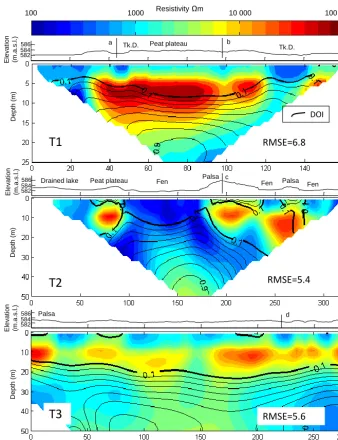
Figure 5. Elevation profiles and ERT results for T1, T2, and T3. DOI<0.1 (black lines) indicates that the model is well constrained by the data. Landforms are indicated on top of elevation profiles along T1 and T2 (Tk.D=thermokarst depression) together with coring points in T1 (a is point 3 in Fig. 1, and b is point 4 in Fig. 1) and T3 (d is point 6 in Fig. 1) as well as the 10 m borehole in T2 (c is point 1 in Fig. 1). No landforms are indicated along T3 after the first palsa (0–25 m) due to the complex micro topography of hummocks and thermokarst depressions along this transect.
all transects, allowing the permafrost base to be interpreted only along parts of T2. In contrast, under T1 and T3 the DOI rapidly increases under the peat plateau and hummocks. Due to the wide electrode spacing adopted (2 and 4 m), the per-mafrost table under the active layer is too shallow to be visi-ble in the ERT data.
4.3 Geophysical interpretations
Permafrost occurs under the palsa and peat plateau surfaces along T1 and T2 as well as under the hummocks along T3
0 50 100 150 200 250 275 560
565 570 575 580 585
50 100 150 200 250 300
555 560 565 570 575 580 585
Distance (m)
E
lev
a
tio
n
(m
)
20 40 60 80 100 120 140 160
575 580 585
a b c d e f
a
a
b c
b
g
T3 T2 T1
50 100 150 200 250 300
535 540 545 550 555 560 565 570 575 580
ERT permafrost, 1000-1688 m interval
ERT 1688 m, local best fit
GPR permafrost table uncertainty interval
GPR mineral interface uncertainty interval
GPR permafrost table
GPR mineral interface
50 100 150 200 250 300
535 540 545 550 555 560 565 570 575 580
ERT permafrost, 1000-1688 m interval
ERT 1688 m, local best fit
GPR permafrost table uncertainty interval
GPR mineral interface uncertainty interval
GPR permafrost table
GPR mineral interface ERT talik
ERT permafrost boundary
ERT permafrost GPS ground surface
uncertainty
GPR Talik
Figure 6. Interpreted permafrost distribution along T1, T2, and T3. Uncertainty intervals come from the range of estimated signal velocities
for GPR (Table 1) and from the range of resistivity values (1000–1700m) used for identifying the permafrost boundary for ERT. In sections marked GPR Talik (red dotted line), GPR depth conversions have been made using saturated peat velocities down to the peat–mineral interface (green line) and then using saturated mineral substrate velocities down to the permafrost table (blue line). In the remaining parts of transects, the dry peat velocities have been used down to the permafrost table. No interpretations of ERT data with DOI>0.1 have been made and therefore the permafrost base is only visible along parts of T2. Note the differences in scale in thexdirection between figures and the vertical exaggeration.
Potential taliks (Table 3 and Fig. 6) are numerous and oc-cur in both wet fens, such as all taliks along T2, and rela-tively dry depressions in the terrain, such as all taliks along T1. The sediment cores used for estimating the GPR repre-sentative signal velocity in saturated peat were taken in both a relatively dry location and a wet fen, but the calculated ve-locities were nearly identical, indicating that the soil mois-ture at depth was similar at both locations. Most of T3 was underlain by taliks and these were found under both wet fens and drier surface depressions. The taliks range in depth from 2.1 m (T3f, numbering from Table 3 and Fig. 6) to 6.7 m (T1c) based on the GPR data and are slightly deeper, al-though within the range of uncertainty based on the ERT results. From the ERT data, T1c is in fact interpreted as a potential through-going talik. Talik T1b was only detected
from the ERT data, and taliks T3b–T3d appear as one large talik in the ERT data.
4.4 Calculations of active layer thickness and future thaw rates
Table 2. Range of interpreted depths (m) of active layer, peat–mineral interface, and permafrost base averaged along transects at Tavvavuoma.
T1 T2 T3
Mina Representativeb Maxc Mina Representativeb Maxc Mina Representativeb Maxc
Active layer
Observedd 0.51 0.52 0.56
GPR 0.50 0.53 0.57 0.48 0.51 0.54 0.52 0.56 0.59
Peat–mineral interface
GPR 0.77 0.84 1.14 0.68 0.74 1.01 0.63 0.69 0.93
Permafrost base
ERT – – 15.8 17.3 – –
aGPR: using the estimated minimum velocity (Table 1). ERT: using 1000m resistivity boundary (talik).bGPR: using representative estimate velocity (Table 1). ERT:
using 1700m resistivity value.cGPR: using the estimated maximum velocity (Table 1). ERT using 1000m resistivity boundary (permafrost base).dDepth from manual field measurement using a steel probe.
Table 3. Estimated depths (m) of taliks at deepest point. Numbering
is the same as in Fig. 6.
Talik GPR GPR GPR ERT ERT
mina representativeb maxc mina representativeb
T1a 2.4 2.7 3.4 2.5 3.1
T1b – – – 1.6 2.8
T1c 6.0 6.7 8.3 >4.7 >4.7
T2a 5.4 6.1 7.6 5.4 6.9
T2b 5.3 6.0 7.4 6.9 8.8
T3a 5.3 5.9 7.4 5.8 7.8
T3b 5.7 6.4 8.0 6.3 8.2
T3c 5.1 5.7 7.0 4.8 7.9
T3d 3.1 3.5 4.4 – 4.0
T3e 4.6 5.2 6.4 5.4 7.2
T3f 2.0 2.1 2.2 – 3.8
T3g 3.7 4.1 5.2 5.0 6.8
aGPR: using the estimated minimum velocity (Table 1). ERT: using 1000m resistivity
boundary (talik).bGPR: using representative estimate velocity (Table 1). ERT: using
1700m resistivity value.cGPR: using the estimated maximum velocity (Table 1). ERT using 1000m resistivity boundary (permafrost base).
the aforementioned geophysical interpretation. Furthermore, assuming a 2◦C instantaneous temperature increase at the site, a first-order approximation of the long-term thaw rate was calculated to be 6–8.5 cm yr−1. At this rate, the time to completely thaw permafrost, assuming the estimated aver-age thickness along T2 (15.3 m), was calculated to be 175– 260 years.
5 Discussion
5.1 Permafrost and talik distribution at Tavvavuoma The spatial pattern of permafrost and taliks in Tavvavuoma is closely linked to the distribution of palsas, peat plateaus,
fens, and water bodies. This suggests that local factors, such as soil moisture, groundwater flow, ground ice content, sed-iment distributions, and geomorphology, strongly influence the local ground thermal regime (see e.g., Delisle and Al-lard, 2003; McKenzie and Voss, 2013; Woo, 2012; Zuid-hoff, 2002). The relative elevation of permafrost landforms, as well as permafrost resistivity values and sediment dis-tributions, suggests that there is a large variation in ground ice content in the area. Surface elevations of palsas and peat plateaus are highest along T2 and lowest along T3, indicat-ing a higher ice content of the underlyindicat-ing ground along T2, which is likely related to differences in ground substrates be-tween the transects. Coring (<2 m) across the site and ex-isting borehole descriptions (Ivanova et al., 2011) confirm that the ground contains a larger fraction of coarse glacioflu-vial sand and gravel, which are not susceptible to frost heave, closer to T3 as compared to T2.
taliks are more widespread along T3, as permafrost with a low ice content would have reacted more rapidly to warming in the area.
The calculated thaw rate of 6–8.5 cm yr−1is considerably higher than the ca. 1 cm yr−1 deepening of the active layer observed in the region (Åkerman and Johansson, 2008) and inferred from hydrological records (Lyon et al., 2009). One possible reason for this is that these observations were made in the relatively ice-rich top layer of peat, while for the calcu-lations in this study a medium with higher thermal conductiv-ity and lower ice content was used to represent the lower min-eral sediment layer. The 2◦C instantaneous step change in temperature could have further contributed to the higher thaw rates compared to the ones observed. As thawing is driven by gradients in heat it can be argued that permafrost thaw rates should increase with warmer air temperatures. Consid-ering this, the calculated time of complete permafrost thaw of about 175–260 years can be considered reasonable in at least 1 order of magnitude. However, much more rapid palsa degradation has been observed in the region (Zuidhoff, 2002) due to block and wind erosion processes and thermal influ-ence on palsas from expanding water bodies, and very rapid decay of palsa surface areas has been observed in both south-ern Norway and the Canadian Arctic (Payette et al., 2004; Sollid and Sorbel, 1998). The coupled erosion, hydrological, and thermal processes are not represented in the Stefan equa-tion but can be of great importance for permafrost thaw rates (McKenzie and Voss, 2013; Painter et al., 2013; Zuidhoff, 2002). There is clearly a need for quantification of the rel-ative importance of these processes for permafrost thaw to better understand expected future changes in these environ-ments.
5.2 On the complementary nature of the geophysical techniques
Several previous studies have shown the benefits of combin-ing more than one geophysical technique for mappcombin-ing per-mafrost (e.g., De Pascale et al., 2008; Hauck et al., 2004; Schwamborn et al., 2002); in this study the GPR and ERT data also provided complementary information that allowed for interpretations that would not have been possible by using only one of the two data sets. Of course, combining multiple techniques for inference compounds our estimate uncertain-ties. To attain more precise estimates of depths to the differ-ent interfaces, deeper coring data would have been necessary for both more accurate signal velocity estimates for the GPR and for local resistivity values of the ground materials. The fact that ERT depth estimates are consistently higher than the GPR estimates suggest that either the resistivity boundary value for permafrost is in fact lower than our local estimate, or that GPR signal velocities are higher than the values used in this study. Since our local permafrost resistivity estimate was made in peat at the permafrost table, which can have a
very high ice content compared to deeper sediment layers, it is a more likely explanation for this discrepancy.
GPR and ERT yielded somewhat overlapping data but the two data sets have different strengths and therefore comple-ment each other well. The GPR data worked well for iden-tifying the permafrost table with high confidence, especially in the top 2 m where sediment cores could be easily obtained for validation and signal velocity estimates. This suitability of GPR for identifying permafrost interfaces in the top 1– 2 m has been shown in several studies (e.g., Doolittle et al., 1992; Hinkel et al., 2001; Moorman et al., 2003). The ERT data, using the setup in this study, do not yield data in the up-permost part of the ground and also have higher uncertainty where resistivity contrasts are high (Fig. 5), which makes them less suited for the active layer and shallow taliks. With the ERT data it is, however, possible to image relatively deep in the ground where the GPR cannot penetrate. By combining both GPR and ERT the active layer, the base of permafrost, and potential taliks could be identified along at least parts of the transects, which could not have been achieved with good confidence by either of the two methods alone.
6 Concluding remarks
Peat plateau complexes offer an interesting challenge to the Cryosphere community as they are clear mosaics combining local-scale differences manifested as permafrost variations. As such variation occurs both horizontally and vertically in the landscape, geophysical techniques offer a good possibil-ity to record current permafrost conditions across scales. Fur-thermore, by combining methods, such as GPR and ERT as demonstrated here, complementary and independent views of the permafrost extents can be acquired. The results of this study show a heterogeneous pattern of permafrost extent re-flecting both local and climatic processes of permafrost for-mation and degradation. To improve our understanding of landscape–permafrost interactions and dynamics will require a community effort to benchmark variability across the scales and environments within the pan-Arctic. This is particularly important in lesser-studied regions and across the sporadic permafrost zone where changes are occurring rapidly.
Author contributions. Ylva Sjöberg designed the study, carried out
Acknowledgements. This study was kindly supported by Sveriges
Geologiska Undersökning (SGU), the Bolin Centre for Climate Research, Lagrelius fond, Göran Gustafssons Stiftelse för natur och miljö i Lappland, and Svenska Sällskapet för Antropologi och Geografi. The authors are grateful to Peter Jansson and Britta Sannel for lending us the equipment necessary for this study and to Romain Pannetier, Kilian Krüger, Matthias Siewert, Britta Sannel, and Lars Labba for fieldwork support. We are also grateful to Andrew Parsekian for technical advice on the GPR survey design and María A. García Juanatey for consultation when processing the ERT data.
Edited by: J. Boike
References
Åkerman, H. J. and Johansson, M.: Thawing permafrost and thicker active layers in sub-arctic Sweden, Permafrost Periglac., 19, 279–292, doi:10.1002/ppp.626, 2008.
Alexandersson, H.: Temperature and precipitation in Sweden 1860– 2001, SMHI, Norrköping, Sweden, 2002.
Arcone, S. A., Lawson, D. E., Delaney, A. J., Strasser, J. C., and Strasser, J. D.: Ground-penetrating radar reflection profiling of groundwater and bedrock in an area of discontinuous permafrost, Geophysics, 63, 1573–1584, doi:10.1190/1.1444454, 1998. Christiansen, H. H., Etzelmuller, B., Isaksen, K., Juliussen, H.,
Far-brot, H., Humlum, O., Johansson, M., Ingeman-Nielsen, T., Kris-tensen, L., Hjort, J., Holmlund, P., Sannel, A. B. K., Sigsgaard, C., Akerman, H. J., Foged, N., Blikra, L. H., Pernosky, M. A., and Odegard, R. S.: The Thermal State of Permafrost in the Nordic Area during the International Polar Year 2007–2009, Permafrost Periglac., 21, 156–181, doi:10.1002/ppp.687, 2010.
Davis, J. L. and Annan, A. P.: Ground-penetrating radar for high-resolution mapping of soil and rock, Geophys. Prospect., 37, 531–551, doi:10.1111/j.1365-2478.1989.tb02221.x, 1989. Delisle, G. and Allard, M.: Numerical simulation of the
tempera-ture field of a palsa reveals strong influence of convective heat transport by groundwater, in: Proceeding of the 8th International Permafrost Conference, 21–25 July 2003, Zurich, Switzerland, 181–186, 2003.
De Pascale, G. P., Pollard, W. H., and Williams, K. K.: Geo-physical mapping of ground ice using a combination of capac-itive coupled resistivity and ground-penetrating radar, North-west Territories, Canada, J. Geophys. Res.-Earth., 113, F02S90, doi:10.1029/2006jf000585, 2008.
Dobinski, W.: Geophysical characteristics of permafrost in the Abisko area, northern Sweden, Pol. Polar Res., 31, 141–158, doi:10.4202/ppres.2010.08, 2010.
Doolittle, J. A., Hardisky, M. A., and Black, S.: A ground-penetrating radar study of Goodstream palsas, Newfoundland, Canada, Arct. Alp. Res., 24, 173–178, doi:10.2307/1551537, 1992.
Fortier, R., LeBlanc, A. M., Allard, M., Buteau, S., and Calmels, F.: Internal structure and conditions of permafrost mounds at Umi-ujaq in Nunavik, Canada, inferred from field investigation and electrical resistivity tomography, Can. J. Earth Sci., 45, 367–387, doi:10.1139/e08-004, 2008.
Gacitua, G., Tamstorf, M. P., Kristiansen, S. M., and Uribe, J. A.: Estimations of moisture content in the active layer in an Arctic ecosystem by using ground-penetrating radar profiling, J. Appl. Geophys., 79, 100–106, doi:10.1016/j.jappgeo.2011.12.003, 2012.
Giesler, R., Lyon, S. W., Mörth, C.-M., Karlsson, J., Karlsson, E. M., Jantze, E. J., Destouni, G., and Humborg, C.: Catchment-scale dissolved carbon concentrations and export estimates across six subarctic streams in northern Sweden, Biogeosciences, 11, 525–537, doi:10.5194/bg-11-525-2014, 2014.
Hauck, C., Vonder Muhll, D., and Maurer, H.: Using DC re-sistivity tomography to detect and characterize mountain per-mafrost, Geophys. Prospect., 51, 273–284, doi:10.1046/j.1365-2478.2003.00375.x, 2003.
Hauck, C., Isaksen, K., Muhll, D. V., and Sollid, J. L.: Geophysical surveys designed to delineate the altitudinal limit of mountain permafrost: An example from Jotunheimen, Norway, Permafrost Periglac., 15, 191–205, doi:10.1002/ppp.493, 2004.
Hinkel, K. M., Doolittle, J. A., Bockheim, J. G., Nelson, F. E., Paetzold, R., Kimble, J. M., and Travis, R.: Detection of subsur-face permafrost features with ground-penetrating radar, Barrow, Alaska, Permafrost Periglac., 12, 179–190, doi:10.1002/ppp.369, 2001.
Hoekstra, P., Selimann, P., and Delaney, A.: Airborne resistivity mapping of permafrost near Fairbanks, Alaska, US Army CR-REL, Hanover, New Hampshire, 51, 1974.
Hugelius, G., Bockheim, J. G., Camill, P., Elberling, B., Grosse, G., Harden, J. W., Johnson, K., Jorgenson, T., Koven, C. D., Kuhry, P., Michaelson, G., Mishra, U., Palmtag, J., Ping, C.-L., O’Donnell, J., Schirrmeister, L., Schuur, E. A. G., Sheng, Y., Smith, L. C., Strauss, J., and Yu, Z.: A new data set for estimating organic carbon storage to 3 m depth in soils of the northern cir-cumpolar permafrost region, Earth Syst. Sci. Data, 5, 393–402, doi:10.5194/essd-5-393-2013, 2013.
Hugelius, G., Strauss, J., Zubrzycki, S., Harden, J. W., Schuur, E. A. G., Ping, C.-L., Schirrmeister, L., Grosse, G., Michaelson, G. J., Koven, C. D., O’Donnell, J. A., Elberling, B., Mishra, U., Camill, P., Yu, Z., Palmtag, J., and Kuhry, P.: Estimated stocks of circumpolar permafrost carbon with quantified uncertainty ranges and identified data gaps, Biogeosciences, 11, 6573–6593, doi:10.5194/bg-11-6573-2014, 2014.
IPCC: Climate Change 2013: The Physical Science Basis, in: Con-tribution of Working Group I to the Fifth Assessment Report of the Intergovernmental Panel on Climate Change, edited by: Stocker, T. F., Qin, D., Plattner, G.-K., Tignor, M., Allen, S. K., Boschung, J., Nauels, A., Xia, Y., Bex, V., and Midgley, P. M., Cambridge University Press, Cambridge, UK and New York, NY, USA, 1535 pp., 2013.
Ishikawa, M., Watanabe, T., and Nakamura, N.: Genetic differences of rock glaciers and the discontinuous mountain permafrost zone in Kanchanjunga Himal, eastern Nepal, Permafrost Periglac., 12, 243–253, doi:10.1002/ppp.394, 2001.
Ivanova, N. V., Kuznetsova, I. L., Parmuzin, I. S., Rivkin, F. M., and Sorokovikov, V. A.: Geocryological Conditions in Swedish Lap-land, in: Proceedings of the 4th Russian Conference on Geocry-ology, 7–9 June 2011, Moscow State University, Moscow, Rus-sia, 77–82, 2011.
re-gion, Hydrol. Earth Syst. Sci., 17, 3827–3839, doi:10.5194/hess-17-3827-2013, 2013.
Joseph, S., Giménez, D., and Hoffman, J. L.: Dielectric permittiv-ity as a function of water content for selected New Jersey soils, New Jersey Geological and Water Survey, Trenton, NJ, available at: http://www.state.nj.us/dep/njgs/geodata/dgs10-1.htm (last ac-cess: 17 December 2013), 2010.
Klingbjer, P. and Moberg, A.: A composite monthly temperature record from Tornedalen in northern Sweden, 1802–2002, Int. J. Climatol., 23, 1465–1494, doi:10.1002/joc.946, 2003.
Kneisel, C., Hauck, C., and Vonder Muhll, D.: Permafrost be-low the timberline confirmed and characterized by geoelec-trical resistivity measurements, Bever Valley, eastern Swiss Alps, Permafrost Periglac., 11, 295–304, doi:10.1002/1099-1530(200012)11:4<295::aid-ppp353>3.0.co;2-l, 2000.
Kneisel, C., Saemundsson, D., and Beylich, A. A.: Reconnaissance surveys of contemporary permafrost environments in central Ice-land using geoelectrical methods: Implications for permafrost degradation and sediment fluxes, Geogr. Ann. A, 89, 41–50, doi:10.1111/j.1468-0459.2007.00306.x, 2007.
Kneisel, C., Emmert, A., and Kästl, J.: Application of 3D elec-trical resistivity imaging for mapping frozen ground conditions exemplified by three case studies, Geomorphology, 210, 71–82, doi:10.1016/j.geomorph.2013.12.022, 2014.
Lewkowicz, A. G., Etzelmuller, B., and Smith, S. L.: Charac-teristics of Discontinuous Permafrost based on Ground Tem-perature Measurements and Electrical Resistivity Tomography, Southern Yukon, Canada, Permafrost Periglac., 22, 320–342, doi:10.1002/ppp.703, 2011.
Loke, M. H.: Rapid 2-D Resistivity & IP inversion using the least-squares method (RES2DINV ver. 3.59 for Windows XP/Vista/7, manual), Geotomo Software, Malaysia, 2010.
Loke, M. H. and Barker, R. D.: Rapid least-squares inver-sion of apparent resistivity pseudosections by a quasi-Newton method, Geophys. Prospect., 44, 131–152, doi:10.1111/j.1365-2478.1996.tb00142.x, 1996.
Lyon, S. W., Destouni, G., Giesler, R., Humborg, C., Mörth, M., Seibert, J., Karlsson, J., and Troch, P. A.: Estimation of permafrost thawing rates in a sub-arctic catchment using re-cession flow analysis, Hydrol. Earth Syst. Sci., 13, 595–604, doi:10.5194/hess-13-595-2009, 2009.
Lyon, S. W., Mörth, M., Humborg, C., Giesler, R., and Destouni, G.: The relationship between subsurface hydrology and dissolved carbon fluxes for a sub-arctic catchment, Hydrol. Earth Syst. Sci., 14, 941–950, doi:10.5194/hess-14-941-2010, 2010.
Marescot, L., Loke, M. H., Chapellier, D., Delaloye, R., Lambiel, C., and Reynard, E.: Assessing reliability of 2D resistivity imag-ing in mountain permafrost studies usimag-ing the depth of investiga-tion index method, Near Surf. Geophys., 1, 57–67, 2003. McKenzie, J. M. and Voss, C. I.: Permafrost thaw in a
nested groundwater-flow system, Hydrogeol. J., 21, 299–316, doi:10.1007/s10040-012-0942-3, 2013.
Moorman, B. J., Robinson, S. D., and Burgess, M. M.: Imaging periglacial conditions with ground-penetrating radar, Permafrost Periglac., 14, 319–329, doi:10.1002/ppp.463, 2003.
Neidell, N. S. and Taner, T. M.: Semblance and other coherency measures for multichannel data, Geophysics, 36, 482–497, 1971.
Nelson, F. E. and Outcalt, S. I.: A computational method for pre-diction and regionalization of permafrost, Arct. Alp. Res., 19, 279–288, doi:10.2307/1551363, 1987.
Oldenburg, D. W. and Li, Y. G.: Estimating depth of investiga-tion in dc resistivity and IP surveys, Geophysics, 64, 403–416, doi:10.1190/1.1444545, 1999.
Painter, S. L., Moulton, J. D., and Wilson, C. J.: Modeling chal-lenges for predicting hydrologic response to degrading per-mafrost, Hydrogeol. J., 21, 221–224, doi:10.1007/s10040-012-0917-4, 2013.
Payette, S., Delwaide, A., Caccianiga, M., and Beauchemin, M.: Accelerated thawing of subarctic peatland permafrost over the last 50 years, Geophys. Res. Lett., 31, L18208, doi:10.1029/2004gl020358, 2004.
Reynolds, J. M.: An Introduction to Applied and Environmental Geophysics, 2nd Edn., John Wiley & Sons, Hoboken, 2011. Riseborough, D., Shiklomanov, N., Etzelmuller, B., Gruber, S., and
Marchenko, S.: Recent advances in permafrost modelling, Per-mafrost Periglac., 19, 137–156, doi:10.1002/ppp.615, 2008. Sandmeier Geophysical Research: ReflexW software
ver-sion 6.1, available at: http://www.sandmeier-geo.de (last access: March 2015), 2012.
Sannel, A. B. K. and Kuhry, P.: Warming-induced destabilization of peat plateau/thermokarst lake complexes, J.Geophys. Res.-Biogeo., 116, 156–181, doi:10.1029/2010jg001635, 2011. Schwamborn, G. J., Dix, J. K., Bull, J. M., and Rachold,
V.: High-resolution seismic and ground penetrating radar-geophysical profiling of a thermokarst lake in the western Lena Delta, northern Siberia, Permafrost Periglac., 13, 259–269, doi:10.1002/ppp.430, 2002.
Seppälä, M.: Synthesis of studies of palsa formation underlining the importance of local environmental and physical characteristics, Quatern. Res., 75, 366–370, doi:10.1016/j.yqres.2010.09.007, 2011.
Sjöberg, Y., Frampton, A., and Lyon, S. W.: Using streamflow char-acteristics to explore permafrost thawing in northern Swedish catchments, Hydrogeol. J., 21, 121–131, doi:10.1007/s10040-012-0932-5, 2013.
Sollid, J. L. and Sorbel, L.: Palsa bogs as a climate indicator – Ex-amples from Dovrefjell, southern Norway, Ambio, 27, 287–291, 1998.
Tarnocai, C., Canadell, J., Mazhitova, G., Schuur, E. A. G., Kuhry, P., and Zimov, S.: Soil organic carbon stocks in the northern circumpolar permafrost region, Global Biogeochem. Cy., 23, GB2023, doi:10.1029/2008GB003327, 2009.
Westermann, S., Wollschläger, U., and Boike, J.: Monitoring of ac-tive layer dynamics at a permafrost site on Svalbard using multi-channel ground-penetrating radar, The Cryosphere, 4, 475–487, doi:10.5194/tc-4-475-2010, 2010.
Woo, M.-K.: Permafrost Hydrology, Springer, Heidelberg, 563 pp., 2012.
Wramner, P.: Studier av palsmyrar i Tavvavuoma och Laivadalen, Lappland – Studies of palsa mires in Tavvavuoma and Laivadalen, Lappland, Licenciate Thesis, Göteborg University, Gothenburg, Sweden, 1968.
Wramner, P., Backe, S., Wester, K., Hedvall, T., Gunnarsson, U., Alsam, S., and Eide, W.: Förslag till övervakningsprogram för Sveriges palsmyrar – Proposed monitoring program for den’s palsa mires, Länsstyrelsen i Norrbottens Län, Luleå, Swe-den, 2012.
Zuidhoff, F. S.: Recent decay of a single palsa in relation to weather conditions between 1996 and 2000 in Laivadalen, north-ern Sweden, Geogr. Ann. A, 84, 103–111, doi:10.1111/1468-0459.00164, 2002.