Global surface-ocean CO 2and sea–air CO2 ﬂux variability from an observation-driven ocean mixed-layer scheme

(1)

Ocean Sci., 9, 193–216, 2013 www.ocean-sci.net/9/193/2013/ doi:10.5194/os-9-193-2013

EGU Journal Logos (RGB)

Advances in

Geosciences

Open Access

Natural Hazards

and Earth System

Sciences

Open Access

Annales

Geophysicae

Open Access

Nonlinear Processes

in Geophysics

Open Access

Atmospheric

Chemistry

and Physics

Open Access

Atmospheric

Chemistry

and Physics

Open Access

Discussions

Atmospheric

Measurement

Techniques

Open Access

Atmospheric

Measurement

Techniques

Open Access

Discussions

Biogeosciences

Open Access Open Access

Biogeosciences

Discussions

Climate

of the Past

Climate

of the Past

Discussions

Earth System

Dynamics

Earth System

Dynamics

Discussions

Geoscientific

Instrumentation

Methods and

Data Systems

Open Access

Geoscientific

Instrumentation

Methods and

Data Systems

Open Access

Discussions

Geoscientific

Model Development

Geoscientific

Model Development

Discussions

Hydrology and

Earth System

Sciences

Open Access

Hydrology and

Earth System

Sciences

Open Access

Discussions

Ocean Science

Discussions

Solid Earth

Discussions

The Cryosphere

Discussions

Natural Hazards

and Earth System

Sciences

Open Access

Discussions

Global surface-ocean

p

CO

2

and sea–air CO

2

flux variability from an

observation-driven ocean mixed-layer scheme

C. R¨odenbeck1, R. F. Keeling2, D. C. E. Bakker3, N. Metzl4, A. Olsen5,6,7, C. Sabine8, and M. Heimann1

1_{Max Planck Institute for Biogeochemistry, Jena, Germany}

2_{Scripps Institution of Oceanography, University of California, San Diego, USA}

3_{School of Environmental Sciences, University of East Anglia, Norwich Research Park, Norwich, UK} 4_{LOCEAN-IPSL, CNRS, Paris, France}

5_{Institute of Marine Research, Bergen, Norway} 6_{Uni Bjerknes Centre, Bergen, Norway}

7_{Bjerknes Centre for Climate Research, Bergen, Norway} 8_{NOAA Pacific Marine Environmental Laboratory, Seattle, USA}

Correspondence to: C. R¨odenbeck ([email protected])

Received: 27 April 2012 – Published in Ocean Sci. Discuss.: 27 June 2012

Revised: 23 January 2013 – Accepted: 29 January 2013 – Published: 1 March 2013

Abstract. A temporally and spatially resolved estimate of

the global surface-ocean CO2 partial pressure field and the sea–air CO2 flux is presented, obtained by fitting a simple data-driven diagnostic model of ocean mixed-layer biogeo-chemistry to surface-ocean CO2 partial pressure data from the SOCAT v1.5 database. Results include seasonal, interan-nual, and short-term (daily) variations. In most regions, es-timated seasonality is well constrained from the data, and compares well to the widely used monthly climatology by Takahashi et al. (2009). Comparison to independent data ten-tatively supports the slightly higher seasonal variations in our estimates in some areas. We also fitted the diagnostic model to atmospheric CO2data. The results of this are less robust, but in those areas where atmospheric signals are not strongly influenced by land flux variability, their seasonality is nev-ertheless consistent with the results based on surface-ocean data. From a comparison with an independent seasonal cli-matology of surface-ocean nutrient concentration, the diag-nostic model is shown to capture relevant surface-ocean bio-geochemical processes reasonably well. Estimated interan-nual variations will be presented and discussed in a compan-ion paper.

1 Introduction

The oceans are considered the dominant player in the global carbon cycle on long timescales, e.g. in the glacial– interglacial cycles (e.g. Sigman and Boyle, 2000). On a multi-millennial timescale, the oceans will be the sink for 80–95 % of the anthropogenic CO2emissions, and 70–80 % on a timescale of several hundred years (Archer et al., 1997). Currently, the oceans take up about 25 % of the emissions (Sarmiento et al., 2010). Concerns exist, however, that the sink efficiency may decrease in the coming decades as a consequence of anthropogenic climate change, as suggested by model projections (e.g. Sarmiento and Le Quéré, 1996; Matear and Hirst, 1999; Joos et al., 1999) and tentatively con-firmed by data analysis (e.g. Le Quéré et al., 2007, 2010). As a prerequisite to understanding the involved processes, one needs to quantify sea–air CO2 fluxes, their variability, and their response to forcing.

Currently, two data streams are used to estimate the vari-ability of sea–air CO2fluxes:

– Based on measurements of the CO2 partial pressure (pCO2_{) of surface water, the sea–air CO}

2 flux is cal-culated through a gas exchange parameterization. As

pCO2 _{measurements only exist at discrete locations}

(2)

194 C. R¨odenbeck et al.: Global surface-oceanpCO2and sea–air CO

2flux variability

proposed: (1) statistical interpolation combined with an advection–diffusion equation (Takahashi et al., 2009); (2) purely statistical interpolation with error quantifica-tion (Jones et al., 2012b); (3) multi-linear regressions betweenpCO2 _{and ocean state variables (e.g. Park et al.,}

2010; Chen et al., 2011); (4) neural networks learn-ing the relationship between pCO2 _{and oceanic state}

variables available from remote sensing platforms and ocean reanalysis projects (e.g. Lef`evre et al., 2005; Tel-szewski et al., 2009); (5) assimilation of thepCO2 _data

into a process model of ocean biogeochemistry (Valsala and Maksyutov, 2010; While et al., 2012). These meth-ods are complementary in certain aspects: the more sta-tistical methods are dominated by the data themselves but are strongly affected by spatial and temporal gaps, while the more complex methods more easily spread the information but are dependent on driver data sets or even on model formulations.

– The CO2exchange between the Earth surface and the at-mosphere can be quantified based on atmospheric CO2 mixing ratio measurements (e.g. Conway et al., 1994) by the atmospheric transport inversion (e.g. Newsam and Enting, 1988; Rayner et al., 1999; Bousquet et al., 2000; R¨odenbeck et al., 2003; Baker et al., 2006) (see Sect. 2.1). This estimation does not involve any param-eterization of gas exchange. However, ocean fluxes are difficult to detect by this method in most parts of the globe, because their imprint on the atmospheric mixing ratio records is small compared to that of the much more variable land fluxes: Even if ocean-internal processes (biology, transport) cause mixed-layer carbon sources and sinks of comparable variability as the land bio-sphere, the resulting sea–air CO2exchange is much less variable and smoothed out in time because the carbon-ate chemistry of seawcarbon-ater slows the equilibration rcarbon-ate of dissolved CO2with the atmosphere. In addition, the re-sponses to warming/cooling partially counteract the ef-fects of ocean-internal sources/sinks. A further problem of atmospheric inversions based on data from a discrete set of measurement sites is that information is only pro-vided on scales comparable to or larger than the distance between the sites or the sampling frequency, while vari-ability exists also on smaller scales.

A further data-based method to estimate sea–air CO2fluxes uses ocean-interior carbon data in inverse calculations of oceanic transport (Gloor et al., 2003; Mikaloff Fletcher et al., 2006). This method is independent of parameterizations of gas exchange as well. However, it only yields long-term sea– air CO2fluxes over large spatial regions, not its temporal or high-resolution spatial variability. The long-term global sea– air CO2 flux has also been estimated from observed trends in atmospheric oxygen (Keeling and Shertz, 1992) as well as from13C isotopic ratios in atmospheric CO2(Ciais et al., 1995).

In view of the above-mentioned problem of the atmospheric CO2inversions, most of these studies use the sea–air flux cli-matology by Takahashi et al. (2009) (or earlier versions) as a Bayesian prior (in some cases, the long-term fluxes from ocean-interior inversions are used in the prior as well, e.g. R¨odenbeck et al. (2003), or formalized as joint inversion by Jacobson et al. (2007)). Out of this context, the data-based sea–air CO2 fluxes presented here have been devel-oped aiming to (1) provide not only a monthly seasonal cy-cle but variability also on short-term (daily) and interannual timescales, (2) use an assimilation scheme that can easily and self-consistently compare or even combine the observational information of atmospheric and surface-ocean data, and (3) use a framework that can be extended to also incorporate con-straints from other tracers, such as oxygen.

The presented results are based on the newly available Sur-face Ocean CO2 Atlas (SOCAT) database (version 1.5) of CO2fugacity measurements (Pfeil et al., 2012, http://www. socat.info/). We describe the estimation method and test its performance, also using independent data. As a first step of analysis, this study mainly focuses on the mean seasonal cy-cle, because on this timescale (1) we can compare to the widely used monthlypCO2 _{climatology by Takahashi et al.}

(2009), (2) we can investigate mutual consistency between the surface-oceanpCO2 _{constraint and that by atmospheric}

CO2data as the signal/noise ratio is large, and (3) we can test the plausibility of our process representations invoking a seasonal surface-ocean phosphate (PO4) climatology. Esti-mated interannual variations of the sea–air CO2flux are pre-sented and discussed in a companion paper (R¨odenbeck et al., 2013).

2 Method

2.1 Concept – overview

In a classical atmospheric inversion, a spatio-temporal field of surface-to-atmosphere carbon fluxes is estimated such that its corresponding mixing ratio field – as simulated by an at-mospheric tracer transport model – matches as closely as possible a set of mixing ratio observations. The match is gauged by a quadratic cost function to be minimized (Ap-pendix A2).

Here we extend the inversion framework by not only con-sidering the process of atmospheric transport but also pro-cesses in the oceanic mixed layer: The atmospheric trans-port model is supplemented by a chain of parameterizations of gas exchange, carbonate chemistry, and a carbon bud-get equation, which determine the sea-to-air CO2exchange (fCO2

(3)

C. R¨odenbeck et al.: Global surface-oceanpCO2_{and sea–air CO}

2flux variability 195

22 C. R¨odenbeck et al.: Sea-airCO2flux estimated fromCO2partial pressure data

Atm. mixing ratio [ppm]: cCO2₍_i,t₎

meteo.,fneeCO2,ffosCO2 →

K

Atm. Transport

Sea-air fluxes [mol/m2

/s]: fCO2

ma (x,y,t)

u,T,S,pbaro_,_XCO2 _→

K

Solub., Gas exch.

Mixed-layer partial press. [µatm]: pCO2(x,y,t)

T,S,A,γDIC,pCO2

,Ref

m ,C

DIC,Ref

m →

K

Carbon. chem.

Mixed-layer concentration [µmol/kg]: C_mDIC(x,y,t)

h →

K

C Budget

Ocean-internal sources/sinks [mol/m2_/_s_]: _fDIC

int (x,y,t)

Fig. 1. Summary of the main quantities and process

parameteriza-tions involved in the diagnostic ocean mixed-layer model. Thick boxes denote the process parameterizations given in Sect. 2.2, each expressing the quantity right above as a function of the quantity right below. Quantities at the arrows on the left represent driver data entering the parameterizations. See Table 2 for mathematical symbols, and Appendix A1 for the equations and further explana-tion.

Atm. Inv. For ATM For SFC

cCO2

obs⇐⇒

Jc

cCO2 _cCO2

obs⇐⇒

Jc

cCO2

K

AT

K

AT

→fCO2

ma f CO2 ma f CO2 ma K GE K GE

pCO2 _pCO2 obs⇐⇒

Jp

pCO2

K CC K CC CDIC m C DIC m K CB K CB

→fDIC

int →f

DIC

int

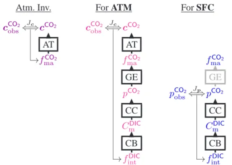
Fig. 2. Illustration of the inverse procedure (three modi). Boxes

de-note the process parameterizations from Figure 1, causally linking quantities from bottom to top. Double arrows symbolize the match-ing between observed and modelled quantities, as gauged by a cost functionJ (Appendix A2). Thin arrows indicate the adjustments of the respective unknowns done to minimize the model-data mis-match. Left: Pure atmospheric transport inversion not used here but given for reference: The sea-air fluxesfCO2

ma are adjusted to match atmospheric mixing ratios (terrestrial Net Ecosystem Exchange is adjusted as well but omitted from this schematic for clarity). Mid-dle: In case ATM, ocean-internal sources/sinksfDIC

int are adjusted instead of sea-air fluxes to match atmosphericCO2mixing ratios

(again Net Ecosystem Exchange is further adjusted). Right: In case SFC, ocean-internal sources/sinks are adjusted to match the surface-oceanCO2partial pressure observations. Sea-air fluxes are

then calculated from the estimated partial pressure field.

Fig. 1. Summary of the main quantities and process

parameteriza-tions involved in the diagnostic ocean mixed-layer model. Thick boxes denote the process parameterizations given in Sect. 2.2, each expressing the quantity right above as a function of the quantity right below. Quantities at the arrows on the left represent driver data entering the parameterizations. See Table 2 for mathematical sym-bols, and Appendix A1 for the equations and further explanation.

the individual processes impose spatial and temporal struc-ture to the sea–air fluxes, based on the spatio-temporal infor-mation from the driver data (sea-surface temperature (SST), wind speed, etc., Fig. 1). (2) The explicit representation of oceanic processes involves further quantities, notably sea-surface CO2 partial pressure. Through cost function contri-butions gauging the match of modelled and measuredpCO2_,

these data can be used as an observational constraint replac-ing the atmospheric data (Fig. 2, right). In this mode of op-eration, atmospheric transport models and atmospheric data are actually no longer used in the inverse calculation, but the Bayesian framework, including a-priori spatial and temporal correlations, is still applied in the same way as in the atmo-spheric mode.

The calculation is global over the time period 1985–2011, with a temporal resolution of 1 day and a horizontal resolu-tion of approximately 4◦latitude×5◦longitude (TM3 model grid).

2.2 Process parameterizations

All processes considered explicitly are given in Fig. 1 and summarized in the following. Details, including the equa-tions used, are found in Appendix A.

Atmospheric transport. Atmospheric CO2 mixing ratio fields in response to surface-to-atmosphere fluxes are simu-lated by the global off-line atmospheric transport model TM3 (Heimann and K¨orner, 2003) with a spatial resolution of≈4◦ lat.×5◦ long.×19 vertical levels. The model is driven by 6-h interannual meteorological fields derived from the Na-tional Centers for Environmental Prediction (NCEP)

reanal-22 C. R¨odenbeck et al.: Sea-airCO2flux estimated fromCO2partial pressure data

Atm. mixing ratio [ppm]: cCO2(i,t)

meteo.,fneeCO2,f

CO2

fos →

K

Atm. Transport

Sea-air fluxes [mol/m2

/s]: f_maCO2(x,y,t)

u,T,S,pbaro_,_XCO2 _→

K

Solub., Gas exch.

Mixed-layer partial press. [µatm]: pCO2(x,y,t)

T,S,A,γDIC,pCO2m ,Ref,C

DIC,Ref

m →

K

Carbon. chem.

Mixed-layer concentration [µmol/kg]: C_mDIC(x,y,t)

h →

K

C Budget

Ocean-internal sources/sinks [mol/m2_/

s]: f_intDIC(x,y,t)

Fig. 1. Summary of the main quantities and process

parameteriza-tions involved in the diagnostic ocean mixed-layer model. Thick boxes denote the process parameterizations given in Sect. 2.2, each expressing the quantity right above as a function of the quantity right below. Quantities at the arrows on the left represent driver data entering the parameterizations. See Table 2 for mathematical symbols, and Appendix A1 for the equations and further explana-tion.

Atm. Inv. For ATM For SFC

cCO2 obs⇐⇒

Jc

cCO2 _cCO2

obs⇐⇒

Jc

cCO2

K

AT

K

AT

→fCO2

ma f CO2 ma f CO2 ma K GE K GE

pCO2

obs⇐⇒

Jp

pCO2

K CC K CC CDIC m C DIC m K CB K CB

→fDIC

int →f

DIC int

Fig. 2. Illustration of the inverse procedure (three modi). Boxes

de-note the process parameterizations from Figure 1, causally linking quantities from bottom to top. Double arrows symbolize the match-ing between observed and modelled quantities, as gauged by a cost functionJ (Appendix A2). Thin arrows indicate the adjustments of the respective unknowns done to minimize the model-data mis-match. Left: Pure atmospheric transport inversion not used here but given for reference: The sea-air fluxesfCO2

ma are adjusted to match atmospheric mixing ratios (terrestrial Net Ecosystem Exchange is adjusted as well but omitted from this schematic for clarity). Mid-dle: In case ATM, ocean-internal sources/sinksfDIC

int are adjusted instead of sea-air fluxes to match atmosphericCO2mixing ratios

(again Net Ecosystem Exchange is further adjusted). Right: In case SFC, ocean-internal sources/sinks are adjusted to match the surface-oceanCO2partial pressure observations. Sea-air fluxes are

then calculated from the estimated partial pressure field.

Fig. 2. Illustration of the inverse procedure (three modi). Boxes

denote the process parameterizations from Fig. 1, causally linking quantities from bottom to top. Double arrows symbolize the match-ing between observed and modelled quantities, as gauged by a cost functionJ (Appendix A2). Thin arrows indicate the adjustments of the respective unknowns done to minimize the model–data mis-match. Left: pure atmospheric transport inversion not used here but given for reference: the sea–air fluxesfCO2

ma are adjusted to match atmospheric mixing ratios (terrestrial net ecosystem exchange is ad-justed as well but omitted from this schematic for clarity). Middle: in the case of ATM, ocean-internal sources/sinksf_intDICare adjusted instead of sea–air fluxes to match atmospheric CO2mixing ratios (again net ecosystem exchange is further adjusted). Right: in the case of SFC, ocean-internal sources/sinks are adjusted to match the surface-ocean CO2partial pressure observations. Sea–air fluxes are then calculated from the estimated partial pressure field.

ysis (Kalnay et al., 1996). The model fields are sampled at the location and time of the individual mixing ratio measure-ments used. TM3 has performed well in intercomparisons of state-of-the-art global tracer transport models (e.g. Stephens et al., 2007; Law et al., 2008).

Solubility and gas exchange. Diffusive sea-to-air gas

ex-change is proportional to the over-/undersaturation of CO2in the surface ocean and to the piston velocity with the quadratic wind speed dependence by Wanninkhof (1992), scaled to match the global average piston velocity of Naegler (2009) (Appendix A1.1).

Carbonate chemistry. The carbon species relevant for gas

exchange (CO2) only account for a small part of the car-bon relevant in the ocean-internal budget (dissolved inor-ganic carbon, DIC). The link between CO2abundance (ex-pressed in terms of partial pressure pCO2

m ) and DIC abun-dance (in terms of its concentration C_mDIC) is determined by chemical equilibria, which we assume to be attained in-stantaneously. The non-linear dependence ofpCO2

(4)

196 C. R¨odenbeck et al.: Global surface-oceanpCO2and sea–air CO

2flux variability

Mixed-layer carbon budget. Changes in the

spatio-temporal field of dissolved inorganic carbon in the ocean mixed layer need to be balanced by the sum of fluxes (Ap-pendix A1.3). As the sea–air flux itself depends on carbon concentration, this balance can be expressed as a linear first-order differential equation. Its solution gives DIC concen-trationC_mDICas a function of the ocean-internal sinksf_intDIC

(representing the total effect of biological conversion and vertical/horizontal advection/diffusion on mixed-layer car-bon concentration). An additional important item in the bud-get is the re-entrainment during mixed-layer deepening of carbon left behind previously during mixed-layer shoaling, which we represent as a “history flux”fhist. We further con-sider the influence of freshwater fluxes.

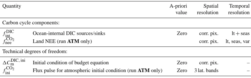
2.3 Main adjustable degrees of freedoms

The ocean-internal carbon sources and sinks (f_intDIC) at the end of the described chain of process parameterizations is the basic unknown to be adjusted to match the surface-ocean

pCO2 _{or atmospheric CO}

2 data (next section). It is treated similarly to the unknown sea–air flux in the pure atmospheric transport inversion (Fig. 2), including Bayesian a-priori spa-tial and temporal correlations. The detailed specification and further explanations are found in Appendix A2.2.

2.4 Data constraints – base runs

We will present results of two cases that differ in the data set used as main constraint (Fig. 2):

SFC. In the main case used to create the primary

prod-uct of this study, the ocean part of the diagnostic scheme is fit to surface pCO2 _{data points from the SOCAT v1.5}

database (Pfeil et al., 2012, http://www.socat.info/). Data pre-treatment and further details are given in Table 1. SOCAT data cover about 6 million pixels/time steps globally within the calculation period (until 2007, see Supplement Figs. S7.3 and S7.4 for data distribution).

ATM. As a comparison case used to assess the consistency

between surface-ocean and atmospheric data, the diagnostic scheme is fit to atmospheric CO2mixing ratios measured ap-proximately weekly or hourly at a set of sites by various in-stitutions. Details are given in Table 1.

3 Results and discussion

The main product of this study is a data-based estimate of the global spatio-temporal CO2partial pressure field and ul-timately the sea–air CO2 fluxes. Here we characterize and evaluate its robustness, errors, and information content. In addition, we compare these results with independent data and previous estimates. The consideration of interannual vari-ations is done in the companion paper (R¨odenbeck et al., 2013).

3.1 Overview

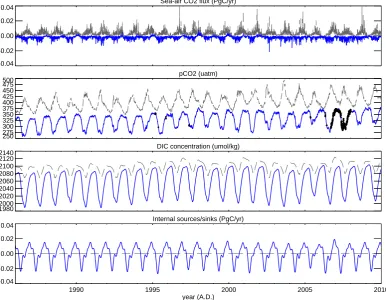
To illustrate the characteristics of the quantities and the tem-poral scales involved in the scheme, Fig. 3 shows time se-ries of key quantities (as of run SFC, blue) at the exam-ple pixel around Station M in the Norwegian Sea (66◦_N,

2◦E). The ocean-internal sources/sinks (bottom panel) are relatively smooth, as the a-priori temporal correlations (Ap-pendix A2.2) suppress fast variations. The mixed-layer DIC concentration (panel above) responds to these ocean-internal fluxes and the emerging sea–air exchange. Being their tem-poral integral, the DIC concentration is slightly shifted in phase with respect to the ocean-internal fluxes. In addition, the DIC concentration is rising in response to the atmo-spheric CO2 increase. The surface-ocean CO2 partial pres-sure (3rd panel from bottom) shares the rise and the varia-tions with the DIC concentration, but the seasonality is again slightly shifted because of the temperature and alkalinity ef-fects. Finally, the sea–air CO2flux (top panel) is dominated by thepCO2 _{variability; in addition, it shows high-frequency}

(daily) variability due to wind speed and solubility changes. Figure 3 also illustrates the dampening effect of the carbon-ate chemistry on sea–air exchange, as the seasonal amplitude of the sea–air flux (top) is much lower than that of the ocean-interior flux (bottom).

The spatial resolution and domain of the calculation is il-lustrated by Fig. 4, showing the amplitude of the mean sea-sonal cycle ofpCO2 _{for each pixel.}

3.2 Data and model constraints

The estimatedpCO2_{and sea–air CO}

2flux fields combine in-formation from the partial pressure data and from the pro-cess parameterizations. To illustrate this, Fig. 3 also shows the a-priori state (thin dashed grey) defined byf_{int, pri}DIC =0 (Appendix A2.2, see bottom panel). The choicef_{int, pri}DIC =0 means that, without data knowledge, it is equally likely to have an internal source or an internal sink at any given lo-cation and time, and thus corresponds to a state of no infor-mation onf_intDIC. The variations in the prior values ofC_mDIC,

pCO2_{, and the sea–air fluxes}_fCO2

ma , which then follow from the process parameterizations, only comprise responses to variations in sea surface temperature and the other driving variables (including rising atmospheric CO2), but miss vari-ations in the ocean-internal sources/sinks. As this a-priori

pCO2 _{field contradicts the data (black dots), the estimation}

procedure now adjusts the internal fluxf_intDICin such a way that the data are matched as closely as possible (blue). Most prominently, this reduces or – as at the example pixel of Fig. 3 – even reverses the seasonal variations ofpCO2

(re-flecting that thermal, biological, and physical effects partially oppose each other). The fit at further locations is given below (Sect. 3.4).

(5)

C. R¨odenbeck et al.: Global surface-oceanpCO2and sea–air CO

C. R¨odenbeck et al.: Sea-airCO2flux estimated fromCO2partial pressure data 23

Sea-air CO2 flux (PgC/yr)

-0.04 -0.02 0.00 0.02 0.04

pCO2 (uatm)

250 275 300 325 350 375 400 425 450 475 500

DIC concentration (umol/kg)

1980 2000 2020 2040 2060 2080 2100 2120 2140

Internal sources/sinks (PgC/yr)

1990 1995 2000 2005 2010

year (A.D.) -0.04

-0.02 0.00 0.02 0.04

Fig. 3. Example time series (full daily resolution) at the model pixel at around Station M (66◦_{N, 2}◦_{E) of the main quantities of the diagnostic}

model (Figure 1): Sea-airCO2fluxes (f CO2

ma ), surface-oceanCO2partial pressure (p CO2

m ), mixed-layerDICconcentration (C

DIC

m ), as well as

ocean-internal carbon addition to (removal from) the mixed layer (fDIC

int). Estimates have been obtained by fitting the diagnostic scheme to

SOCAT surface-oceanCO2partial pressure data (SFC, blue). The SOCAT data points that happen to fall in the example pixel are shown as

black dots in thepCO2

m panel. The Bayesian prior (f

DIC

int = 0and correspondingC

DIC

m ,p

CO2

m , andf

CO2

ma, Appendix A2.2, Sect. 3.2) is also given

(thin dashed gray).

Fig. 4. Amplitude of the seasonal cycle of surface-oceanCO2

par-tial pressure (µatm) estimated by fitting the diagnostic scheme to the SOCAT data (run SFC). The amplitude is given as temporal standard deviation of the 1997-2009 monthly meanpCO2

m at each

pixel.

Fig. 3. Example time series (full daily resolution) at the model pixel around Station M (66◦N, 2◦E) of the main quantities of the diagnostic model (Fig. 1): sea–air CO2fluxes (fmaCO2), surface-ocean CO2partial pressure (pmCO2), mixed-layer DIC concentration (CmDIC), as well as ocean-internal carbon addition to (removal from) the mixed layer (f_intDIC). Estimates have been obtained by fitting the diagnostic scheme to SOCAT surface-ocean CO₂partial pressure data (SFC, blue). The SOCAT data points that happen to fall in the example pixel are shown as black dots in thepCO2

m panel. The Bayesian prior (fintDIC=0 and correspondingCmDIC,pCOm 2, andfmaCO2, Appendix A2.2, Sect. 3.2) is also given (thin dashed grey lines).

C. R¨odenbeck et al.: Sea-air

CO

2

flux estimated from

CO

2

partial pressure data

23

Sea-air CO2 flux (PgC/yr)

-0.04

-0.02

0.00

0.02

0.04

pCO2 (uatm)

250

275

300

325

350

375

400

425

450

475

500

DIC concentration (umol/kg)

1980

2000

2020

2040

2060

2080

2100

2120

2140

Internal sources/sinks (PgC/yr)

1990

1995

2000

2005

2010

year (A.D.)

-0.04

-0.02

0.00

0.02

0.04

Fig. 3. Example time series (full daily resolution) at the model pixel at around Station M (66

◦

N, 2

◦

E) of the main quantities of the diagnostic

model (Figure 1): Sea-air

CO

2

fluxes (f

CO₂

ma

), surface-ocean

CO

2

partial pressure (p

CO₂

m

), mixed-layer

DIC

concentration (C

DIC

m

), as well as

ocean-internal carbon addition to (removal from) the mixed layer (f

intDIC

). Estimates have been obtained by fitting the diagnostic scheme to

SOCAT surface-ocean

CO

₂

partial pressure data (SFC, blue). The SOCAT data points that happen to fall in the example pixel are shown as

black dots in the

p

CO2

m

panel. The Bayesian prior (f

DIC

int

= 0

and corresponding

C

DIC

m

,

p

CO₂

m

, and

f

CO₂

ma

, Appendix A2.2, Sect. 3.2) is also given

(thin dashed gray).

Fig. 4. Amplitude of the seasonal cycle of surface-ocean

CO

2

par-tial pressure (µ

atm

) estimated by fitting the diagnostic scheme to

the SOCAT data (run SFC). The amplitude is given as temporal

standard deviation of the 1997-2009 monthly mean

p

CO2

m

at each

Fig. 4. Amplitude of the seasonal cycle of surface-ocean CO2partial pressure (µatm) estimated by fitting the diagnostic scheme to the SOCAT data (run SFC). The amplitude is given as temporal standard deviation of the 1997–2009 monthly meanpCO2

m at each pixel.

(6)

198 C. R¨odenbeck et al.: Global surface-oceanpCO2and sea–air CO

2flux variability 24 C. R¨odenbeck et al.: Sea-airCO2flux estimated fromCO2partial pressure data

Constrained Extrapolated

pixel pixel

fCO2

ma f

CO2 ma

K

GE

K

GE

pCO2 obs⇐⇒

Jp

pCO2 _pCO2

K

CC

K

CC

CDIC

m C

DIC

m

K

CB

correlated

K

CB

→fDIC

int −→ f

DIC

int

adjustments

Fig. 5. Illustration of the information flow in the spatio-temporal

extrapolation through a-priori correlations. Where data values ex-ist, pixels are directly constrained (left column, which is identical to Figure 2). Due to the a-priori spatial correlations (Appendix A2.2), adjustments tofDIC

int at the constrained pixel also change f

DIC

int at neighbouring unconstrained pixels. pCO2 _{is then calculated}

pas-sively from the extrapolatedfDIC

int by the process parameterizations, using the local values of the driving fields (right column).

In data-dense areas, local adjustments tofDIC

int (both for constrained and for extrapolated pixels) will need to compromise between sev-eral data constraints within the correlation radius (de-weighted with distance due to the decay of the correlation, Figure 13). As with any smoothing, this may be beneficial in suppressing outliers, but also adverse in partly suppressing small-scale signals (the structures from the driving data of the parameterizations are never smoothed however, as the smoothing only acts onfDIC

int). In data-poor areas, there may exist pixels that do not have any constrained pixel within the correlation radius; thenfDIC

int will stay close to the prior. In time, extrapolation happens not only due to the a-priori correla-tions, but additionally due to the memory effect resulting from the relaxation time of the budget equation Eq. (A21).

Fig. 5. Illustration of the information flow in the spatio-temporal

extrapolation through a-priori correlations. Where data values ex-ist, pixels are directly constrained (left column, which is identical to Fig. 2). Due to the a-priori spatial correlations (Appendix A2.2), adjustments tof_intDICat the constrained pixel also changef_intDICat neighbouring unconstrained pixels.pCO2 _{is then calculated}

pas-sively from the extrapolatedf_intDICby the process parameterizations, using the local values of the driving fields (right column).

In data-dense areas, local adjustments tof_intDIC(both for constrained and for extrapolated pixels) will need to compromise between sev-eral data constraints within the correlation radius (de-weighted with distance due to the decay of the correlation, Fig. A1). As with any smoothing, this may be beneficial in suppressing outliers, but also adverse in partly suppressing small-scale signals (the structures from the driving data of the parameterizations are never smoothed however, as the smoothing only acts onf_intDIC). In data-poor areas, there may exist pixels that do not have any constrained pixel within the correlation radius; thenf_intDICwill stay close to the prior. In time, extrapolation happens not only due to the a-priori correla-tions, but additionally due to the memory effect resulting from the relaxation time of the budget equation Eq. (A21).

regular sampling, as at Station M since 2006, are a rare ex-ception). Thus, only a small fraction of pixels/time steps is constrained directly in the described way. However, most parts of the space–time domain are still constrained indi-rectly through extrapolation via the spatial and temporal a-priori correlations defined in Appendix A2.2. The mecha-nism is illustrated in Fig. 5. In particular, as seasonal vari-ations inf_intDICare allowed to be adjusted much more freely than non-seasonal variations (equivalent to a-priori correla-tions between adjustments tof_intDICat any given day of year in each year, Appendix A2.2), the mean seasonal cycle is ex-trapolated throughout the time period of the calculation. This also means that data points in any year can contribute to con-strain this mean seasonality. Thus, though there are regions or periods too far away from data points for extrapolation, larger-scale seasonal variations are constrained almost every-where in the ocean. This has been confirmed by assessing how well a givenpCO2 _{field can be retrieved by the scheme}

from pseudo data sampled from this field at the times and lo-cations of the SOCAT data (Appendix B). Constraining inter-annual variations requires more even data distribution in time than constraining seasonal variability; this density of data is only available is some areas of the ocean (R¨odenbeck et al., 2013).

The spatio-temporal a-priori correlations also act to smoothf_intDICon small scales (Fig. 3, bottom), as they damp small-scale and short-term variations. This has been done because the available data do not have the spatial or tem-poral density required to constrain these fine-scale features adequately. Nevertheless, despite the smoothf_intDICthe corre-spondingpCO2 _{and sea–air CO}

2flux fields (Fig. 3, top) do comprise fast variations as represented in the process param-eterizations, including responses to variations in temperature (changes in solubility and chemical equilibrium) or in wind speed (e.g. accelerated depletion of an oversaturated mixed layer in a high wind speed event, Bates et al., 1997). These effects already account for a considerable part of short-term variations (see Sect. 3.4 below). Only variations related to fast ocean-internal processes, such as the sub-weekly varia-tions of upwelling events or algal blooms, will be missing. In any case, the pseudo-data tests (Appendix B) confirm that the degrees of freedom in the diagnostic scheme provide suffi-cient flexibility to follow variability as contained in thepCO2

fields from a biogeochemical process model simulation (as the model has less day-to-day variability than the realpCO2

field, however, this test may underestimate errors from alias-ing such high-frequency variations into variations on the re-solved timescales).

3.3 Robustness

Figures 6 and 7 show the seasonality of the sea–air CO2 flux and the surface-ocean CO2partial pressure as estimated from SOCAT data by run SFC. The fields have been inte-grated/averaged over a set of regions splitting the ocean into basins and latitude bands.

To test how robustly the results are determined from the data and to assess the impact of errors in the parameteri-zations and their driving fields, individual important model elements have been changed in sensitivity runs: (i) increase and decrease of the a-priori uncertainty by a factor 2, leav-ing more/less freedom for inverse adjustments, (ii) decrease of the a-priori uncertainty of non-seasonal variations inf_intDIC

by a factor of 2, (iii) increase in the spatial correlation lengths by a factor of 3, (iv) increase and decrease of the global mean piston velocity by 3.2 cm (range given by Naegler, 2009), and (v) increase and decrease mixed-layer depthhby a factor of 2. The resulting range of results (grey bands in Figs. 6 and 7) is generally very narrow compared to the seasonal ampli-tude, in particular forpCO2_{. In most regions, the sensitivity of}

the sea–air flux is slightly larger than that ofpCO2_{, almost}

(7)

C. R¨odenbeck et al.: Global surface-oceanpCO2and sea–air CO

Fig. 6. Monthly mean seasonal cycle of sea–air CO2fluxes, esti-mated by fitting the diagnostic scheme to SOCAT data (run SFC, blue). The grey shading around the standard result comprises sen-sitivity cases listed in Sect. 3.3. Fluxes have been integrated over latitude bands split into ocean basins (including open ocean, coastal areas and marginal seas; panels in geographical arrangement). Sea-sonal cycles have been calculated over the period 1997–2009; the first half year is repeated for clarity.

is found mostly in the North Pacific and the temperate North Atlantic, entirely due to a few marginal areas (including pix-els in the far north of the Pacific, or the Black Sea and the Caspian Sea added to the Atlantic region, see Fig. 4) where thepCO2 _{seasonality is exceptionally high due to high SST}

seasonality, but where gas exchange is low such that their contribution to regional sea–air flux is nevertheless small. If

pCO2 _{is averaged only over the open ocean, the}_pCO2 _spread

becomes narrow in all regions (see Supplement Fig. S7.8).

3.4 Fit to the data

The match of the estimatedpCO2 _{field and measured data}

points somewhat depends on the considered location (Fig. 8). At the North Pacific example pixel (i.e. within the region of largest spread among the sensitivity cases in Fig. 7), the sea-sonality is underestimated by some µatm. This may result

Fig. 7. Analogously to Fig. 6, monthly mean seasonal cycle of

surface-ocean carbon dioxide partial pressurepCO2

m , estimated by fitting the diagnostic scheme to SOCAT data (run SFC, blue). The grey shading comprises the same sensitivity cases. For comparison, thepCO2

m climatology by Takahashi et al. (2009) is given (violet, with a small additive adjustment to transfer the nominal year 2000 average into a 1997–2009 average according to the rising atmo-spheric CO₂partial pressure fieldpCO2

a , Eq. A3).

(8)

200 C. R¨odenbeck et al.: Global surface-oceanpCO2and sea–air CO

SOCAT Data Independent Data (not in SOCAT v1.5)

N Pacific (155W,55N)

1996 1998 2000 2002 2004 year (A.D.)

200 225 250 275 300 325 350 375 400 425 450 475

pCO2 (uatm)

BTM (64W,32N)

2006 2007 2008

year (A.D.) 300

325 350 375 400 425 450

pCO2 (uatm)

STM (2E,66N)

2006 2007 2008

year (A.D.) 275

300 325 350 375 400

pCO2 (uatm)

Stratus (85.62W,19.70S)

2007 2008 2009 2010

year (A.D.) 325

350 375 400 425 450

pCO2 (uatm)

Fig. 8. Comparison between the estimatedpCO2_{field (run SFC, blue) and measurements (black dots) at test locations. Left: Data contained}

in SOCAT v1.5 (larger dots) at a pixel in the North Pacific, and the pixel around Station M in the North Atlantic. Right: Two mooring sites in the North Atlantic (BTM, (64◦_W,32◦_{N)) and South Pacific (Stratus (85.62}◦_W,19.70◦_{S)) by Sabine et al. (2010) that are not part}

of SOCAT v1.5 (smaller dots). ThepCO2_{field has been picked at the times where the measurements exist (connected by straight lines for}

clarity); the time axes have been limited to respective years with data. The monthly climatology by Takahashi et al. (2009) (regridded and with added trend parallel to the atmosphericCO2increase, violet) is also given. See Supplementary material for comparisons to SOCAT data

(Figure S7.5) and independent data (Figure S7.6) at further locations.

0 0.01 0.02 0.03 0.04 0.05

-100 -50 0 50 100

Rel. frequency (1/uatm)

pCO2 difference (uatm) Winter (JFM) Histogram

Gaussian Summer (JAS) Histogram Gaussian

Fig. 9. Histograms of the residuals of the fit to SOCAT data (i.e., pCO2_{estimated by run SFC minus data, µ}_atm_{, horizontal axis).}

Thin lines show the relative abundance (within bins of5µatm) of residuals over all pixels from the North Pacific (North of 45◦_{N) and}

all time steps with data in winter (Jan-Feb-Mar, blue) or in summer (Jul-Aug-Sep, red). Respective thick lines give a Gaussian of the same mean and standard deviation. See Supplementary material, Figure S5.2 for global maps of seasonal residuals.

Fig. 8. Comparison between the estimatedpCO2field (run SFC, blue) and measurements (black dots) at test locations. Left: data contained in

SOCAT v1.5 (larger dots) at a pixel in the North Pacific, and the pixel around Station M in the North Atlantic. Right: two mooring sites in the North Atlantic (BTM, 32◦N, 64◦W) and South Pacific (Stratus, 19.70◦S, 85.62◦W) by Sabine et al. (2010) that are not part of SOCAT v1.5 (smaller dots). ThepCO2 _{field has been picked at the times where the measurements exist (connected by straight lines for clarity); the time}

axes have been limited to respective years with data. The monthly climatology by Takahashi et al. (2009) (regridded and with added trend parallel to the atmospheric CO2increase, violet) is also given. See Supplement for comparisons to SOCAT data (Fig. S7.5) and independent data (Fig. S7.6) at further locations.

26 C. R¨odenbeck et al.: Sea-airCO2flux estimated fromCO2partial pressure data

SOCAT Data Independent Data (not in SOCAT v1.5)

N Pacific (155W,55N)

1996 1998 2000 2002 2004

year (A.D.) 200

225 250 275 300 325 350 375 400 425 450 475

pCO2 (uatm)

BTM (64W,32N)

2006 2007 2008

year (A.D.) 300

325 350 375 400 425 450

pCO2 (uatm)

STM (2E,66N)

2006 2007 2008

year (A.D.) 275

300 325 350 375 400

pCO2 (uatm)

Stratus (85.62W,19.70S)

2007 2008 2009 2010

year (A.D.) 325

350 375 400 425 450

pCO2 (uatm)

Fig. 8. Comparison between the estimatedpCO2_{field (run SFC, blue) and measurements (black dots) at test locations. Left: Data contained}

in SOCAT v1.5 (larger dots) at a pixel in the North Pacific, and the pixel around Station M in the North Atlantic. Right: Two mooring sites in the North Atlantic (BTM, (64◦_W,32◦_{N)) and South Pacific (Stratus (85.62}◦_W,19.70◦_{S)) by Sabine et al. (2010) that are not part}

of SOCAT v1.5 (smaller dots). ThepCO2 _{field has been picked at the times where the measurements exist (connected by straight lines for}

clarity); the time axes have been limited to respective years with data. The monthly climatology by Takahashi et al. (2009) (regridded and with added trend parallel to the atmosphericCO2increase, violet) is also given. See Supplementary material for comparisons to SOCAT data

(Figure S7.5) and independent data (Figure S7.6) at further locations.

0 0.01 0.02 0.03 0.04 0.05

-100 -50 0 50 100

Rel. frequency (1/uatm)

pCO2 difference (uatm) Winter (JFM) Histogram

Gaussian Summer (JAS) Histogram Gaussian

Fig. 9. Histograms of the residuals of the fit to SOCAT data (i.e., pCO2

estimated by run SFC minus data, µatm, horizontal axis). Thin lines show the relative abundance (within bins of5µatm) of residuals over all pixels from the North Pacific (North of 45◦_{N) and}

all time steps with data in winter (Jan-Feb-Mar, blue) or in summer (Jul-Aug-Sep, red). Respective thick lines give a Gaussian of the same mean and standard deviation. See Supplementary material, Figure S5.2 for global maps of seasonal residuals.

Fig. 9. Histograms of the residuals of the fit to SOCAT data (i.e.

pCO2 _{estimated by run SFC minus data, µatm, horizontal axis).}

Thin lines show the relative abundance (within bins of 5 µatm) of residuals over all pixels from the North Pacific (north of 45◦N) and all time steps with data in winter (January–February–March, blue) or in summer (July–August–September, red). Respective thick lines give a Gaussian of the same mean and standard deviation. See Sup-plement Fig. S5.2 for global maps of seasonal residuals.

but misses any interannual anomalies). See the Supplement (Sect. S5, Figs. S7.5 and S7.6) for more comparisons and statistics.

In order to validate the high-frequency variations, we com-pare them to mooring observations independent of the

SO-CAT v1.5 data set (Fig. 10, upper panels). In the extra-tropics (example sites BSO or MOSEAN+WHOTS), many short-term features are reproduced in run SFC, though mostly with reduced amplitude. Discrepancies (e.g. beginning of 2007 at BSO) can largely be explained by the deviation of sea surface temperature in our driving field – regridded to the≈4◦×5◦ pixels around the stations – from the local temperature (lower panels). Note that this discrepancy does not preclude that the pixel average ofpCO2_{is actually reproduced more accurately}

than the local value, to the extent that our SST field repre-sents the pixel’s average temperature; however, this cannot be validated or falsified based on the point data.

In contrast to the extra-tropics, the high-frequency varia-tions in our estimate are unrelated or even opposite to those of the measurements in the tropics (example site TAO170W), even though the SST field performs similarly as at the extra-tropical sites. While in the extra-tropics warmer SST leads to higher pCO2

m as reproduced by the solubility and chemistry parameterizations, tropicalpCO2

m increases during cold events, as in the upwelling of cold and carbon-rich deep water. Such events would have to be reproduced as high-frequency variations in the ocean-internal sources/sinks

f_intDIC, which however cannot be constrained from the SO-CAT data set (potentially except at very few locations in pe-riods of high-frequency sampling).

(9)

C. R¨odenbeck et al.: Global surface-oceanpCO2and sea–air CO

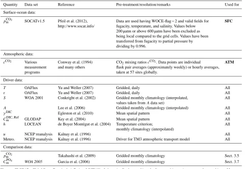
Table 1. Data sets used as constraints or as driver data in the process parameterizations (Sect. A1).

Quantity Data set Reference Pre-treatment/resolution/remarks Used for

Surface-ocean data:

pCO2

m SOCATv1.5 Pfeil et al. (2012), Data are used having WOCE-flag = 2 and valid fields for SFC

http://www.socat.info/ fugacity, temperature, and salinity. Values below 200 µatm or above 600 µatm have been excluded as being local compared to the grid cells. Values have been transferred from fugacity to partial pressure by dividing by 0.996.

Atmospheric data:

cCO2 _Various _{Conway et al. (1994)} _CO

2mixing ratioscCO2. Data points are individual ATM

measurement and many others flask pair averages (approximately weekly) or hourly averages, programs taken at 57 sites globally.

Driver data:

T OAFlux Yu and Weller (2007) Gridded, daily All

ε OAFlux Yu and Weller (2007) Gridded, daily All

S WOA 2001 Conkright et al. (2002) Gridded monthly climatology (interpolated, All values taken fromAdata set)

A Lee et al. (2006) Gridded monthly climatology (interpolated) All

γDIC Egleston et al. (2010) Mean spatial pattern All

CmDIC,Ref GLODAP Key et al. (2004) Mean spatial pattern All

h LOCEAN de Boyer Mont´egut et al. (2004) Temperature criterion; All monthly climatology (interpolated)

u NCEP reanalysis Kalnay et al. (1996) All

Meteo. NCEP reanalysis Kalnay et al. (1996) Driver for TM3 atmospheric transport model All

Comparison data:

pCO2

m Takahashi et al. (2009) Gridded monthly climatology Sect. 3.5

CPO4

m WOA 2005 Garcia et al. (2006) Gridded monthly climatology Sect. 3.7

Glossary: GLODAP = Global Ocean Data Analysis Project; LOCEAN = Laboratoire d’océanographie et du climat: expérimentations et approches numériques; Meteo. = Meteorological variables as listed in Heimann and Körner (2003); NCEP = National Centers for Environmental Prediction; OAFlux = Objectively Analysed air–sea Fluxes; SOCAT = Surface Ocean CO2Atlas; WOCE = World Ocean Circulation Experiment; WOA = World Ocean Atlas; Math symbols see Table 2.

chemistry. In the tropics, more realistic short-term variations could potentially be obtained by parameterization of fast pro-cesses (upwelling events) inf_intDIC.

3.5 Comparison to the Takahashi climatology

The monthly mean seasonal cycle calculated from our spatio-temporal pCO2 _{field has been compared to the widely}

used observation-based climatology by Takahashi et al. (2009), which differs from our method in thepCO2 _{data set}

used (Lamont-Doherty Earth Observatory (LDEO) database, Takahashi et al., 2010) and in the way of spatio-temporal ex-trapolation of the point data into pixels without data: while the diagnostic scheme extrapolates the internal flux field

f_intDICand then inferspCO2 _{from it via the process}

represen-tations (Fig. 5), Takahashi et al. (2009) extrapolates thepCO2

field itself, using a 2-dimensional advection–diffusion

equa-tion1. In data-dense areas, results should not depend much on the extrapolation method.

In most regions, the seasonal cycle estimated from SO-CAT by the diagnostic scheme is similar in phase to the

pCO2 _{climatology by Takahashi et al. (2009) (Fig. 7), though}

the seasonal amplitude is somewhat larger in many regions. Even better agreement is found when only considering the open ocean: the open-ocean seasonalities in the temperate North Pacific and Atlantic almost fully coincide (Supplement Fig. S7.8). Open-ocean agreement is also confirmed at sev-eral of our test locations (Fig. 8).

Differences between our seasonalities and the Takahashi et al. (2009) climatology are somewhat bigger in areas of low data density (e.g. the Southern Ocean), as expected. Com-parison to data at typical test locations tends to confirm the slightly larger seasonal amplitudes in our estimate (Fig. 8 1_{As a further methodological difference, the diagnostic scheme}

(10)

202 C. R¨odenbeck et al.: Global surface-oceanpCO2and sea–air CO

2flux variability

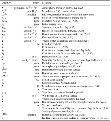
Table 2. Mathematical symbols (also see Table 3). Some quantities are indexed by species or other distinctions explained in the text.

Quantity Unita Meaning

A ppm (µmol m−2s−1)−1 Atmospheric transport matrix, Eq. (A25) CDIC_m µmol kg−1 Mixed-layer DIC concentration

CDIC_a µmol kg−1 DIC concentration in equilibrium with atmosphere cobs ppm Set of observed atmospheric mixing ratios c_mod ppm Modelled mixing ratios, Eq. (A25) c0 ppm Initial mixing ratio

fma µmol m−2s−1 Sea-to-air tracer flux, Eq. (A17) fhist µmol m−2s−1 History (re-entrainment) flux, Eq. (A20) fint µmol m−2s−1 Ocean-internal tracer sources/sinks, Eq. (A18)

F µmol m−2s−1 Flux model matrix, Eq. (A26)

f µmol m−2s−1 Vector of flux discretized at pixels/time steps h m Mixed layer depth

J 1 Cost function, Eq. (A27)

Jc 1 Cost function, atmospheric data part, Eq. (A24)

Jp 1 Cost function, surface-ocean data part, Eq. (A30)

k m s−1 Piston velocity, Eq. (A2)

L mol kg−1atm−1 Solubility (including fugacity correction), Eqs. (A1) and (S1.1) pm µatm Partial pressure in mixed layer, Sect. A1

pa µatm Atmospheric partial pressure, Eq. (A3) pbaro atm Barometric pressure at ocean surface pdry atm Dry-air pressure at ocean surface

pH2O _µatm _{Saturation water vapor pressure above ocean, Eq. (S1.3)}

S ‰ Mixed-layer salinityb

Sc 1 Schmidt number, Appendix S1.1

T ◦C Mixed-layer temperature (sea surface temperature, SST)

t s Time coordinate

ti,te s Start time, end time of inversion period u m s−1 Wind speed at 10 m above surface x 1 Vector of adjustable parameters, Eq. (A26)

X ppm Dry-air molar mixing ratio in the atmosphere above the ocean z m Vertical coordinate

β 1 Temperature factor of CO2partial pressure, Eqs. (A5) and (A6) 0 1 Scaling of piston velocities, Eq. (A2)

γDIC µmol kg−1 Buffer factor (response factor), Eq. (A11)

ε 1 Ice-free fraction of ocean surface (0=ice-covered, 1=ice-free)

a_{ppm = µmol mol}−1_;b_{for the present purposes, salinity in ‰ or on the Practical Salinity Scale are considered interchangeable.}

and Supplement Figs. S7.5 and S7.6). In particular, in the North Pacific where differences between the two methods are biggest, larger seasonalities are confirmed both at the in-dividual pixels (see Fig. 8 for a typical example) and in the larger seasonal bias of about 8.5 µatm in the differences be-tween Takahashi et al. (2009) and SOCAT data points in that area (however, the largest contribution to the difference in the

pCO2 _{average of Fig. 7 comes from the northernmost pixels}

where data are too sparse for a conclusive validation). Data at Station M (Fig. 8) also confirm larger seasonality in the North Atlantic.

Differences between the two estimates are also bigger to-wards the coast. Note that part of these coastal differences come from the fact that, in order to cover the entire ocean surface, we extrapolated the Takahashi et al. (2009)

clima-tology using its open-ocean values. For example, this con-tributes to the differences in the temperate North Atlantic due to the Mediterranean (see Supplement, Fig. S7.5).

Partly, the differences in Fig. 7 can be traced to the fact that the two estimates are based on differentpCO2 _{data sets,}

(11)

C. R¨odenbeck et al.: Global surface-oceanpCO2and sea–air CO

C. R¨odenbeck et al.: Sea-airCO2flux estimated fromCO2partial pressure data 27

BSO (19.5E,72.5N)

2007 year (A.D.) 250

275 300 325 350 375

pCO2 (uatm)

MOSEAN+WHOTS (157.92W,22.77N)

2008 2009

year (A.D.) 325

350 375 400 425

pCO2 (uatm)

TAO170W (170W,2S)

2006 year (A.D.) 375

400 425 450 475 500

pCO2 (uatm)

BSO (19.5E,72.5N)

2007 year (A.D.) 2

4 6 8 10 12

SST (degrC)

MOSEAN+WHOTS (157.92W,22.77N)

2008 2009

year (A.D.) 22

24 26 28

SST (degrC)

TAO170W (170W,2S)

2006 year (A.D.) 24

26 28 30

SST (degrC)

Fig. 10. Top: Time series of surface-oceanpCO2_(µ

atm) at independent mooring sites (not part of SOCATv1.5): Barents Sea Opening (72.5◦_N,19.5◦_{E, Arthun et al. (2012)), combined MOSEAN and WHOTS moorings (22.77}◦_N,157.92◦_{W, Sabine et al. (2010)), and from}

the TAO array (2◦_S,170◦_{W, Sabine et al. (2010)). Comparison between the measurements (black dots) and the}_pCO2_{field estimated by}

fitting to the SOCAT data (blue). The estimated field has been picked at the times where measurements exist; one year as been selected for each site. Bottom: Sea surface temperature measured simultaneously withpCO2_{(black dots) compared to our SST driving field at this pixel}

(light grey).

Fig. 10. Top: time series of surface-oceanpCO2_{(µatm) at independent mooring sites (not part of SOCATv1.5): Barents Sea Opening (72.5}◦_N,

19.5◦E, Arthun et al., 2012), combined MOSEAN and WHOTS moorings (22.77◦N, 157.92◦W, Sabine et al., 2010), and from the TAO array (2◦S, 170◦W, Sabine et al., 2010). Comparison between the measurements (black dots) and thepCO2 _{field estimated by fitting to}

the SOCAT data (blue). The estimated field has been picked at the times where measurements exist; one year has been selected for each site. Bottom: sea surface temperature measured simultaneously withpCO2_{(black dots) compared to our SST driving field at this pixel (light}

grey).

Beyond seasonality, agreement is also found in the im-plied long-term average global sea–air flux. The 1990–2009 average from run SFC is −1.2 PgC yr−1 _{(range between}

−0.95 PgC yr−1and−1.45 PgC yr−1due to sensitivity cases with lower/higher gas exchange rate, Sect. 3.3). Within un-certainties, this agrees well with the value of (−1.36±

0.6)PgC yr−1 recomputed from Takahashi et al. (2009) by Wanninkhof et al. (2012, Table 2, “Net flux” and “Coastal area”) using CCMP winds (Atlas et al., 2011).

In summary, we take the similarity between the seasonali-ties from the two methods based on similar data as an indica-tion that the estimatedpCO2_{field in most regions is informed}

by the data and not primarily method-dependent.

3.6 Comparison ofpCO2-based and atmospheric

results

Figure 11 compares the SOCAT-based fit from Fig. 6 (run

SFC) with the fit of the diagnostic scheme to atmospheric

CO2 data (run ATM). In the Southern Hemisphere, there is broad agreement in the phasing and amplitude of the sea-sonal cycle. In particular, the difference between the two runs is much smaller than their differences from the (common) prior, i.e. than the adjustments due to the respective data con-straints. Less agreement is found in the tropics and the North-ern Hemisphere, in particular in the temperate latitudes.

The ocean fluxes estimated from the atmospheric data are much less robust (more sensitive to changes in uncer-tain model details, not shown) than those estimated from the

pCO2 _{data. As investigated by synthetic data testing}

(Supple-ment Sect. S4), this is largely related to the additional degrees of freedom in adjusting land-to-atmosphere fluxes: signals in the atmospheric data are partially wrongly attributed to land or ocean. Consistently, best agreement between ATM and

SFC occurs in the southern regions away from land

influ-ence, while the large disagreement in the temperate North Pacific is due to the short but strong sink period during sum-mer, more typical for terrestrial boreal ecosystems.

The results establish that oceanic and atmospheric data are consistent in regions away from land influences, but that estimates based on pCO2 _{data provide much stronger}

con-straints on internal ocean processes, in particular in ocean ar-eas closer to land. Combining the oceanic and atmospheric constraints is therefore both possible and beneficial (com-pare Jacobson et al., 2007). It can be implemented by adding together the cost function contributions ofpCO2 _{data (from}

(12)

204 C. R¨odenbeck et al.: Global surface-oceanpCO2_{and sea–air CO}

Pacific 45N-90N -1.5 -1.0 -0.5 0.0 0.5 1.0 1.5 Pacific 15N-45N -1.5 -1.0 -0.5 0.0 0.5 1.0 1.5 Pacific 15S-15N -1.5 -1.0 -0.5 0.0 0.5 1.0 1.5

Sea-air CO2 flux (PgC/yr) Pacific 45S-15S

-1.5 -1.0 -0.5 0.0 0.5 1.0 1.5 Pacific 90S-45S

Jan Jul Jan Jul -1.5 -1.0 -0.5 0.0 0.5 1.0 1.5 Atlantic 45N-90N -1.5 -1.0 -0.5 0.0 0.5 1.0 1.5 Atlantic 15N-45N -1.5 -1.0 -0.5 0.0 0.5 1.0 1.5 Atlantic 15S-15N -1.5 -1.0 -0.5 0.0 0.5 1.0 1.5 Atlantic 45S-15S -1.5 -1.0 -0.5 0.0 0.5 1.0 1.5 Atlantic 90S-45S

Jan Jul Jan Jul -1.5 -1.0 -0.5 0.0 0.5 1.0 1.5 Prior

Fit to SOCAT

Fit to atmospheric CO2

Indian 15S-30N -1.5 -1.0 -0.5 0.0 0.5 1.0 1.5 Indian 45S-15S -1.5 -1.0 -0.5 0.0 0.5 1.0 1.5 Indian 90S-45S

Jan Jul Jan Jul -1.5 -1.0 -0.5 0.0 0.5 1.0 1.5

Fig. 11. Monthly mean seasonal cycle of sea-airCO2fluxes as

Fig-ure 6. Estimates by fitting the diagnostic scheme to SOCAT data (run SFC, blue) are compared to the fit of the scheme to atmospheric CO2mixing ratio data (run ATM, magenta), as well as to the prior

(no data constraint, thin dashed gray).

Pacific 45N-90N -0.5 -0.4 -0.3 -0.2 -0.1 0.0 0.1 0.2 0.3 0.4 0.5 Pacific 15N-45N -0.2 -0.1 0.0 0.1 0.2 Pacific 15S-15N -0.2 -0.1 0.0 0.1 0.2

PO4 concentration (umol/kg) Pacific 45S-15S

-0.2 -0.1 0.0 0.1 0.2 Pacific 90S-45S

Jan Jul Jan Jul -0.2 -0.1 0.0 0.1 0.2 Atlantic 45N-90N -0.2 -0.1 0.0 0.1 0.2 Atlantic 15N-45N -0.2 -0.1 0.0 0.1 0.2 Atlantic 15S-15N -0.2 -0.1 0.0 0.1 0.2 Atlantic 45S-15S -0.2 -0.1 0.0 0.1 0.2 Atlantic 90S-45S

Jan Jul Jan Jul -0.2 -0.1 0.0 0.1 0.2 PO4 climatology

Fit to SOCAT

Indian 15S-30N -0.2 -0.1 0.0 0.1 0.2 Indian 45S-15S -0.2 -0.1 0.0 0.1 0.2 Indian 90S-45S

Jan Jul Jan Jul -0.2

-0.1 0.0 0.1 0.2

Fig. 12. Mixed-layer phosphate concentration (monthly

climatol-ogy, mean subtracted). Seasonality inferred from the SOCAT fit (blue) assumes all ocean-internal carbon sources and sinks are re-lated to phosphate sources and sinks in Redfield proportions. For comparison, the PO4 climatology from the World Ocean Atlas

(WOA, Garcia et al., 2006) is given (green). The grey uncertainty band around the SOCAT-based estimates again gives the range of sensitivity cases as in Figure 7; note however that calculatedPO4is

also sensitive to several further model elements not included in this range.

Fig. 11. Monthly mean seasonal cycle of sea–air CO2 fluxes as Fig. 6. Estimates by fitting the diagnostic scheme to SOCAT data (run SFC, blue) are compared to the fit of the scheme to atmospheric CO2mixing ratio data (run ATM, magenta), as well as to the prior (no data constraint, thin dashed grey)

3.7 Plausibility of the ocean-internal carbon sources and sinks

As the diagnostic scheme (in run SFC) is constructed to match the CO2 partial pressure data, any errors in the pa-rameterizations linking pCO2 _and_fDIC

int (namely carbonate chemistry (including temperature or alkalinity dependence), or mixed-layer carbon budget (including freshwater and his-tory fluxes), see Fig. 1) will be compensated by spurious ad-ditional adjustments to the ocean-internal carbon sources and sinks. On the one hand, this means that the estimatedpCO2

(and sea–air flux) fields will be only little affected by im-perfections in these parameterizations. Even at pixels not di-rectly constrained by apCO2 _{data value but only indirectly}

via extrapolation of thef_intDICfield through its a-priori spatio-temporal correlations (Fig. 5), any such bias will largely can-cel out (to the extent that it is the same at the directly con-strained and the extrapolated pixels). This leads to the robust-ness of thepCO2 _{estimate shown in Sect. 3.3. Therefore, as}

28 C. R¨odenbeck et al.: Sea-airCO₂_{flux estimated from}CO₂_{partial pressure data}

Pacific 45N-90N -1.5 -1.0 -0.5 0.0 0.5 1.0 1.5 Pacific 15N-45N -1.5 -1.0 -0.5 0.0 0.5 1.0 1.5 Pacific 15S-15N -1.5 -1.0 -0.5 0.0 0.5 1.0 1.5

Sea-air CO2 flux (PgC/yr) Pacific 45S-15S

-1.5 -1.0 -0.5 0.0 0.5 1.0 1.5 Pacific 90S-45S

Jan Jul Jan Jul -1.5 -1.0 -0.5 0.0 0.5 1.0 1.5 Atlantic 45N-90N -1.5 -1.0 -0.5 0.0 0.5 1.0 1.5 Atlantic 15N-45N -1.5 -1.0 -0.5 0.0 0.5 1.0 1.5 Atlantic 15S-15N -1.5 -1.0 -0.5 0.0 0.5 1.0 1.5 Atlantic 45S-15S -1.5 -1.0 -0.5 0.0 0.5 1.0 1.5 Atlantic 90S-45S

Jan Jul Jan Jul -1.5 -1.0 -0.5 0.0 0.5 1.0 1.5 Prior

Fit to SOCAT

Fit to atmospheric CO2

Indian 15S-30N -1.5 -1.0 -0.5 0.0 0.5 1.0 1.5 Indian 45S-15S -1.5 -1.0 -0.5 0.0 0.5 1.0 1.5 Indian 90S-45S

Jan Jul Jan Jul -1.5 -1.0 -0.5 0.0 0.5 1.0 1.5

Fig. 11. Monthly mean seasonal cycle of sea-airCO2fluxes as

Fig-ure 6. Estimates by fitting the diagnostic scheme to SOCAT data (run SFC, blue) are compared to the fit of the scheme to atmospheric CO2mixing ratio data (run ATM, magenta), as well as to the prior

(no data constraint, thin dashed gray).

Pacific 45N-90N -0.5 -0.4 -0.3 -0.2 -0.10.0 0.1 0.2 0.3 0.4 0.5 Pacific 15N-45N -0.2 -0.1 0.0 0.1 0.2 Pacific 15S-15N -0.2 -0.1 0.0 0.1 0.2

PO4 concentration (umol/kg) Pacific 45S-15S

-0.2 -0.1 0.0 0.1 0.2 Pacific 90S-45S

Jan Jul Jan Jul -0.2 -0.1 0.0 0.1 0.2 Atlantic 45N-90N -0.2 -0.1 0.0 0.1 0.2 Atlantic 15N-45N -0.2 -0.1 0.0 0.1 0.2 Atlantic 15S-15N -0.2 -0.1 0.0 0.1 0.2 Atlantic 45S-15S -0.2 -0.1 0.0 0.1 0.2 Atlantic 90S-45S

Jan Jul Jan Jul -0.2 -0.1 0.0 0.1 0.2 PO4 climatology

Fit to SOCAT

Indian 15S-30N -0.2 -0.1 0.0 0.1 0.2 Indian 45S-15S -0.2 -0.1 0.0 0.1 0.2 Indian 90S-45S

Jan Jul Jan Jul -0.2

-0.1 0.0 0.1 0.2

Fig. 12. Mixed-layer phosphate concentration (monthly

climatol-ogy, mean subtracted). Seasonality inferred from the SOCAT fit (blue) assumes all ocean-internal carbon sources and sinks are re-lated to phosphate sources and sinks in Redfield proportions. For comparison, the PO4 climatology from the World Ocean Atlas

(WOA, Garcia et al., 2006) is given (green). The grey uncertainty band around the SOCAT-based estimates again gives the range of sensitivity cases as in Figure 7; note however that calculatedPO4is

also sensitive to several further model elements not included in this range.

Fig. 12. Mixed-layer phosphate concentration (monthly

climatol-ogy, mean subtracted). Seasonality inferred from the SOCAT fit (blue) assumes all ocean-internal carbon sources and sinks are re-lated to phosphate sources and sinks in Redfield proportions. For comparison, the PO₄ climatology from the World Ocean Atlas (WOA, Garcia et al., 2006) is given (green). The grey uncertainty band around the SOCAT-based estimates again gives the range of sensitivity cases as in Fig. 7; note however that calculated PO4is also sensitive to several further model elements not included in this range.

long as we are only interested in thepCO2 _{(and sea–air flux)}

fields,f_intDICcould be just considered a mathematical device in the mapping ofpCO2_.

On the other hand, if the ocean-internal fluxes are of inter-est themselves (or in the envisaged extensions of the scheme using further data streams like oxygen coupled to carbon via

(13)

C. R¨odenbeck et al.: Global surface-oceanpCO2and sea–air CO

seasonality is broadly similar in phase and amplitude to the observations (Fig. 12), including characteristic region-to-region differences, though overestimation is seen especially in the temperate latitudes. Given that part of the mismatch arises because the modelled PO4concentration neglects non-Redfieldian sources/sinks (as justified in Appendix C) and because of errors in the observed PO4climatology which are likely significant (and amplified by the Redfield ratio), we take this agreement as broad confirmation of the employed parameterizations.

The carbonate chemistry parameterization (including its driving fields, in particular alkalinity) can specifically be checked using DIC data. This is done in the companion paper (R¨odenbeck et al., 2013).

3.8 The diagnostic mixed-layer scheme in the context of otherpCO2

m mapping methods

The suitability of individualpCO2

m mapping methods (Sect. 1) depends on the intended application. The primary motivation of the diagnostic mixed-layer scheme presented here was to be able to process different data streams (so farpCO2 _and

atmospheric CO2 mixing ratio) in a consistent way, and to combine them. The intention was to achieve this in a data-dominated way, with the least complex model possible.

Statistical methods like the referencepCO2

m climatology by Takahashi et al. (2009) or the interpolation by Jones et al. (2012b) have the advantage of being data-dominated, quite independent of driver data sets and process parameteriza-tions. Regression methods (multi-linear regression, neural networks) use driver data sets to bring in information about modes of variability not resolved by the data, thus addressing the problem of data sparsity; still, they leave flexibility in the way of howpCO2

m and these driving fields are related. Finally, data assimilation into process models then also prescribes this relation analytically, which brings in process knowledge as a further constraint, with the risk of suppressing real vari-ability not captured in the chosen parameterizations.

The diagnostic scheme is similar to the regression meth-ods, thereby also reproducing some of the short-term vari-ability (Sect. 3.4). It is more rigid, like data assimilation, for some processes that may be considered relatively well known (sea–air gas exchange, carbonate chemistry, and mixed-layer mass conservation). It is more free, on the other hand, for the ocean-internal sources and sinks (it is independent of any as-sumptions except for smoothness as needed to regularize the mathematics), i.e. it is purely statistical here. The smoothness assumption represents the mechanism of spatio-temporal in-terpolation2.

2_{This results in different notions of output resolution: Formally,}

the resolution is daily and≈4◦×5◦pixels, but part of this fine-scale variability is only coming from the driving data, while only the larger scales (>monthly and>1500 km areas) are actually in-formed by the SOCAT data.

An advantage of explicit parameterizations, as in the pro-posed mixed-layer scheme, is that the unknowns (here: in-ternal sources/sinks) are physical quantities which are poten-tially open for interpretation (compare Sect. 3.7). They also enable us to use measurements of further quantities of the scheme (such as mixed-layer DIC concentration, nutrients, etc.) as data constraints as well. These further data streams can either be used instead of the present ones (pCO2

m or at-mospheric data) to create alternative estimates for compari-son, or in conjunction with the present ones to potentially in-troduce further unknowns and so distinguish more processes (e.g. carbonate chemistry).

All carbon sources/sinks in the ocean and on land are linked to oxygen sinks/sources, most of them in rather well-defined stoichiometric ratios. The diagnostic scheme can therefore be extended to also make use of atmospheric or oceanic measurements of oxygen (R¨odenbeck et al., 2013).

Beyond the scheme as presented here, multi-linear re-gression could be brought in by expressing the unknown ocean-internal fluxes as a linear combination of (further) driving variables and then match the data by adjusting time-independent weights. This would make the estimation more similar to data assimilation, with the benefits and risks men-tioned above. Further, instead of linear combinations, pa-rameterizations of the ocean-internal processes involving ad-justable parameters could be used if available. This would also open up the way to use even further data streams, such as ocean color from satellite observation.

4 Summary and conclusions

We presented a temporally and spatially resolved estimate of the global surface-ocean CO2 partial pressure field and the sea–air CO2 flux, obtained on the basis of CO2 partial pressure data from the SOCAT database. In order to inter-polate the point data into a spatio-temporal field and to add short-term variations not constrained from the data, a simple model of surface-ocean biogeochemistry, including represen-tations of sea–air gas exchange, solubility, carbonate chem-istry, mixed-layer DIC budget, and seasonal re-entrainment (“history”), was fitted to the observations. The inverse proce-dure was similar to atmospheric inversion calculations, using spatial and temporal a-priori correlations to extrapolate the data information.

Focusing first on seasonal variations, the following con-clusions were drawn:

– The diagnostic scheme can be robustly fit to SOCAT

pCO2 _{data, to estimate the spatio-temp}