Nonlin. Processes Geophys., 20, 1023–1030, 2013 www.nonlin-processes-geophys.net/20/1023/2013/ doi:10.5194/npg-20-1023-2013
© Author(s) 2013. CC Attribution 3.0 License.
Nonlinear Processes
in Geophysics
Open Access
Modelling and simulation of waves in three-layer porous media
S. R. Pudjaprasetya
Mathematics Department, Institut Teknologi Bandung, Jalan Ganesha 10, Bandung, 40132, Indonesia
Correspondence to: S. R. Pudjaprasetya ([email protected])
Received: 28 June 2013 – Revised: 14 October 2013 – Accepted: 15 October 2013 – Published: 25 November 2013
Abstract. The propagation of gravity waves in an emerged three-layer porous medium is considered in this paper. Based on the assumption that the flow can be described by Darcy’s Law, an asymptotic theory is developed for small-amplitude long waves. This leads to a weakly nonlinear Boussinesq-type diffusion equation for the wave height, with coefficients dependent on the conductivities and depths of each layer. In the limit of equal conductivities of all layers, the equation re-duces to the single-layer result recorded in the literature. The model equations are numerically integrated in the case of an incident monochromatic wave hitting the layers. The results exhibit dissipation and also a downstream net height rise at infinity. Wave transmission coefficient in three-layer porous media with conductivity of mangrove is discussed. Numeri-cally, propagation of an initial solitary wave through a porous medium shows the emergence of wave reflection and trans-mission that both evolve as permanent waves. Additionally we examine the impact of a solitary gravity wave on a porous medium breakwater.
1 Introduction
As reported in Dahdouh-Guebas (2006) and Kathiresan and Rajendran (2006), mangrove forests along coastal areas pro-vide shelter against storms and floods, as well as tsunami. Mangrove belts can absorb wave energy and reduce wave amplitude and velocity. The amount of wave amplitude re-duction in mangroves depends on factors such as water depth, coastal profile, and also mangrove species and mangrove thickness. Due to the complexity of the problems, research on mangrove protection mostly relies on field measurement data from certain areas. For instance, Teh et al. (2009) con-ducted a numerical and experimental study of tsunami mit-igation by mangroves (Avicennia officinalis) on the coast of Penang, Malaysia. Liu et al. (2003) studied flow resis-tance of mangrove trees using a depth-averaged
hydrody-namic numerical model. The model and the vegetative pa-rameter were tested using on-site mangrove data (Kandelia sp.) along Keelung River, Taiwan. Masda et al. (1997) re-ported on the experimental study of mangroves (Kandelia sp.) as a coastal protection in the Tong King delta, Vietnam.
Motivated by the protective function of mangrove in miti-gating high waves, here we develop a study of gravity waves in a three-layer porous medium. The three layers here are leaves, trunks, and roots layers of mangrove forest. Wave in-teraction with non-uniform mangrove has been considered in the following literature. Vo-Luong and Massel (2008) study wave energy dissipation in a three-layer mangrove above ar-bitrary depth. They use velocity potential formulations with dissipation to develop a predictive model for random waves in a non-uniform forest in water of changing depth. Massel et al. (1999) study wave attenuation in mangrove forests con-sisting of roots and trunks.
1024 S. R. Pudjaprasetya: Three-layer porous breakwater
assumption, and we develop an asymptotic model for gravity waves in a rigid isotropic three-layer porous structure.
The organization of this paper is as follows. The govern-ing equations are presented in Sect. 2. In Sect. 3 asymptotic methods are used to derive a simpler set of equations; the wave height is shown to satisfy a Boussinesq equation. It is a diffusion equation with higher-order nonlinear and disper-sion terms. In Sect. 4 a predictor–corrector finite-difference scheme is used to simulate the movement of a monochro-matic wave through the medium. Simulation shows ampli-tude reduction of waves in three-layer porous media. Numer-ical simulations clearly display the nonlinear effect: the ris-ing of water levels at the right ends of rather long porous media. In Sect. 5 we use typical hydraulic conductivity of mangrove to calculate the wave transmission coefficient for a porous belt with certain length. In Sect. 6 we show that the newly derived three-layer Boussinesq model can be com-bined with the Boussinesq equation for free water to simulate a solitary wave passing through a porous medium, in which the predictor–corrector scheme follows through. Conclusions are given in Sect. 7.
2 Governing equations for flow in three-layer porous media
In this section, we formulate the governing equations for free-surface flow in a three-layer porous medium over an in-finitely long horizontal axis. Letη(¯ x,¯ t )¯ denote the free
sur-face elevation measured from the undisturbed water level; see Fig. 1. The porous medium consists of three layers: an upper, middle, and lower layer with thicknesses h¯1, h¯2− ¯h1, and
¯
h3− ¯h2, respectively, denoted as ¯
1=(x,¯ z)¯ | − ¯h1≤ ¯z≤ ¯η(x,¯ t ),¯ x¯∈R , (1)
¯
2=
(x,¯ z)¯ | − ¯h2≤ ¯z≤ − ¯h1,x¯∈R , (2)
¯
3=(x,¯ z)¯ | − ¯h3≤ ¯z≤ − ¯h2,x¯∈R . (3) We assume that each layer ¯i for i=1,2,3 is a rigid isotropic porous medium containing an ideal fluid of depth
¯
h3(x).¯
Inside the porous medium we employ Darcy’s law:
ui= −Ki∇ ¯8i, where 8¯i = P
ρg + ¯z, (4) withKihydraulic conductivity for each layeri=1,2,3, with dimension m/sec. In each of the three layers,¯i mass con-servation requires
∇28¯i=0, in ¯i, for i=1,2,3. (5) Along the free surface, the pressureP is constant and can be taken as zero; we then obtain a boundary condition
¯
81= ¯η, on z¯= ¯η. (6)
length. In Section 6 we show the newly derived three layer Boussinesq model can be combined with
Boussinesq equation for free water for simulating solitary wave passing through a porous media, in 60
which the predictor-corrector scheme follows through. Conclusions are given in Section 7.
2 Governing equations for flow in three-layer porous media
In this section, we formulate the governing equations for free-surface flow in a three-layer porous
medium over an infinitely long horizontal axis. Let¯η(¯x,¯t)denotes the free surface elevation
mea-sured from the undisturbed water level, see Figure 1. The porous medium consist of three layers: 65
upper, middle, and lower layer with thicknesses¯h1,¯h2−¯h1,and¯h3−¯h2, respectively, denoted as
¯ Ω1=
{
(¯x,z¯)|−¯h1≤z¯≤¯η(¯x,¯t),x¯∈ ℜ
}
, (1)
¯
Ω2={(¯x,z¯)|−¯h2≤z¯≤ −¯h1,¯x∈ ℜ}, (2)
¯ Ω3=
{
(¯x,z¯)|−¯h3≤z¯≤ −¯h2,¯x∈ ℜ
}
. (3)
We assume that each layerΩ¯i, fori= 1,2,3is a rigid isotropic porous medium containing an ideal
70
fluid of depth¯h3(¯x).
−¯h
3(¯x)
−¯h
2
−¯h
1
¯
z
¯
x
¯
η(¯x,t¯) ¯ Ω1
¯ Ω2
¯ Ω3
Fig. 1.Schematic diagram of the emerged three-layer porous domain.
Inside the porous medium we employ Darcy’s law
ui=−Ki∇Φ¯i, where Φ¯i=
P
ρg+ ¯z, (4)
withKiis hydraulic conductivity, for each layeri= 1,2,3, with dimension m/sec. In each of the
75
three layersΩ¯imass conservation requires
∇2Φ¯i= 0, inΩ¯i, fori= 1,2,3. (5)
3
Fig. 1. Schematic diagram of the emerged three-layer porous do-main.
Along the two interfaces z¯= − ¯hi the following boundary conditions hold:
¯
8i= ¯8i+1 on z¯= − ¯hi for i=1,2, (7) Ki8¯i¯z=Ki+18¯i+1¯z on z¯= − ¯hi for i=1,2. (8) Equation (7) comes from continuity of the pressureP, while Eq. (8) comes from the assumption that fluid influx and out-flux across the interface are the same. The kinematic bound-ary condition along the surface is
¯
ηt¯−K18¯1x¯η¯x¯+K18¯1z¯=0 on z¯= ¯η. (9) Along the impermeable bottomz¯= − ¯h3(x), the normal flux¯
vanishes:
¯
83z¯=0 on z¯= − ¯h3(x).¯ (10)
We summarize: the governing equations for ideal fluid flow in the three-layer porous media are Eqs. (5–10).
3 Asymptotic expansion method leading to Boussinesq equation
Assuming small amplitude long wavelength, we look for asymptotic solutions 8¯i for i=1,2,3 of the governing Eqs. (6–10). LetLbe typical length of the porous medium,
¯
h3 the fluid depth, anda typical free surface displacement.
Introduce the following non-dimensional variables, written without bars as follows:
¯
η=aη, z¯= ¯h3z, x¯=Lx, t¯=
L2
K1h¯3
t,
¯
hi= ¯h3hi, 8¯i=a8i, for i=1,2,3. (11) Note that conductivityK1 is scaled in the non-dimensional
time variable t, and also that h3≡ ¯h3/h¯3=1. Further, we
denote two small parameters
ε= a ¯
h3
, µ2=
h¯ 3
L
2
. (12)
Under the same assumption, Liu and Wen (1997) implement the asymptotic expansion method for the case of a single
S. R. Pudjaprasetya: Three-layer porous breakwater 1025
layer. In this section we extend this approach for the case of three-layer porous media. Compared to this approach, our approach is more direct. Rewriting the governing Eqs. (6–10) in non-dimensional variables, equations for the first layer are µ281xx+81zz=0 in 1 (13)
81=η on z=εη (14)
µ2(ηt−ε81xηx)+81z=0 on z=εη. (15) The equation for the second layer is
µ282xx+82zz=0 in 2. (16)
The equations for the third layer are
µ283xx+83zz=0 in 3 (17)
83z=0 on z= −h3, (18)
The matching conditions along the two interfacesz= −hi are
8i =8i+1 on z= −hifor i=1,2, (19) Ki8i z=Ki+18i+1z on z= −hi for i=1,2. (20) Further, we restrict to Boussinesq approximation, in which
O(ε)=O(µ2), and look for a solution in the form of the series
8i(x, z, t )=8i0+µ28i1+µ28i2+ · · ·, for i=1,2,3.
We implement the asymptotic expansion method in the nor-malized governing Eqs. (13) and (20), by solving the cor-responding equations layer by layer, starting from the first
O(1) terms, to higher order O(µ2) terms, and further to
O(µ4)terms. Hence, an explicit approximate expression of 8i1fori=1,2,3 can then be obtained; see Eqs. (A5), (A7),
and (A10) in Appendix A, respectively. Substituting the ap-proximate potentials into the interface condition (20) along z= −h2yields the following equation of Boussinesq type:
ηt−µ2Aηxxt=(ηx(B+εR31η))x, (21) with coefficientsAandBdependent on the conductivity and thickness of each layer, or explicitly
B=h1+R21(h2−h1)+R31(h3−h2), (22)
withRij=Ki/Kj fori, j=1,2,3. A=1
2(h2−h1)
2+1
2h
2 1−
1 B
1
6h
3 1+
1
2h1(h2−h1)
2
+R21
h1(h2−h1)−
1 B
1
6(h2−h1)
3+1
2h
2
1(h2−h1)
+R31
h1(h3−h2)−
1 B
1
6(h3−h2)
3+1
2
h
(h2−h1)2
−(h3−h2)2+h21
i
(h3−h2)
o
+R32
(h2−h1)2−
1
Bh1(h2−h1)
2
. (23)
The detail derivation of Eq. (21) is given in Appendix A. The Boussinesq equation above, written in normalized vari-ables, is a model for gravity waves in an emerged three-layer porous medium; it is a diffusive equation with higher-order nonlinearity and dispersion.
The horizontal flux of fluid in the three-layer porous media is given by
Q(x, t )≡ − εη
Z
−h1
81xdz−R21 −h1
Z
−h2
82xdz−R31 −h2
Z
−h3
83xdz. (24)
Since the potential8i for each layer was already approxi-mated, substituting(8i)x, fori=1,2,3 yields the following relation:
Q−µ2CQxx= −(B+εη) ηx, (25) with
C= 1
3Bh
3 1−
R21
B
1
6(h2−h1)
3+1
2h
2
1(h2−h1)
+R31
B
1
3(h3−h2)
3−1
2h2(h2−h1)(h3−h2)
. (26) Hence, Eqs. (21) and (25) are Boussinesq models for grav-ity waves in three-layer porous media. It is interesting to note that the flux and surface displacement equations are only weakly coupled; after solving for the displacement us-ing Eq. (21), the flux can be obtained usus-ing Eq. (25). This is different from the fully coupled equations that arise from the corresponding shallow water (free) flow problem. The rea-son for this can be explained as follows. Under Darcy’s as-sumption, we get boundary condition (14) which gives us the first-order term810(x, t )=η(x, t ). From the asymptotic
ex-pansion framework, the first-order terms of Eq. (19) result in 820(x, t )=810(x, t )=η(x, t ), and further 830(x, t )=
820(x, t )=η(x, t ). Since the first-order term of all potential
8i,i=1,2,3 is just η(x, t ), the leading-order term in the continuity equationηt+Qx=0 is just a diffusion equation with a diffusive term proportional toηxx.
Next, we take a zero test where the three layers reduce to one layer. For this purpose we takeh1=h2=h3for which
K3=K2=K1, then the dispersion coefficient and diffusion
coefficients becomeA=1
3h23 andB=h3 respectively, and
furtherC=1 3h
2
3. Hence, Eqs. (21) and (25) reduce to
ηt−µ2 1 3h
2
3ηxxt=(ηx(h3+εη))x (27) Q−1
3 h
2
3Qxx= −(h3+εη)ηx, (28)
1026 S. R. Pudjaprasetya: Three-layer porous breakwater
4 Wave damping in porous media
Comparing Eqs. (21) and (25) for the three-layer model with the corresponding results (27, 28) for the single layer, it can be seen that waves propagating into three layers behave like those propagating into a single layer. Note that the model developed in this paper is based on the assumption that the waves are long compared to depth. For waves of wavelength comparable with the depth (or shorter), the velocity pro-file would vary significantly with depth, and the single- and three-layer models would likely produce different results.
For small amplitude displacementsη, Eq. (27) can be ap-proximated by the linear diffusion equation
ηt−µ2Aηxxt=Bηxx,
with wave-like solutions of the form expi(kx−ωt ). Substi-tuting this yieldsiω+iωµ2Ak2=Bk2or
k=
s
iω
B−iωµ2A=(1+i)
r
ω 2B
1+iωA
B µ
2
−ω
2A2
B2 µ 4+ · · ·
1/2
≈(1+i)
r
ω 2B.
The relation above means that waves of frequencyω propa-gating into the system decay over a distance on the order of a wavelength'1/ k. The penetration length is strongly depen-dent on wave frequencyω, which is approximately√2B/ω. Numerical solutions to Eq. (21) are obtained using the predictor–corrector MacCormack method. The method has second-order accuracy O(4x2,4t2), with 4x and 4t the partition length of spatial and time variables, respectively. Since there is a combine derivative in term ηxxt, we first
rewrite Eq. (21) as
9t= {ηx(B+εR31η)}x, with 9=η−µ2Aηxx.
The first step in the MacCormack method is the predictor 9jn+1=9jn+ 4t
4x2
n
εR31(ηnj+1−η n j)
2
+ B+εR31ηjn
(ηnj+1−2ηnj+ηnj−1)o. (29) Along the left or right boundary, centre difference is replaced with one-sided difference. The overline indicates predicted values. When the predicted values9jn+1 forj=1,· · ·, N x are known, the predicted valuesηnj+1forj=1,· · ·, N xcan be obtained by solving the linear relation Dη=9, with
DN x×N x =IN x×N x−µ2 A
4x2
0 0 0 · · ·0
1−2 1 · · ·0 ..
. . .. . .. . .. ... 0 · · · 1 −2 1 0 · · · 1 −2 1
. (30)
Having
Ψ
nj+1, for
j
= 1
,
···
,N x
we can directly compute
η
jn+1for the new time step, using
η
=
D
−1Ψ
.
200
η
Fig. 2.A periodic tidal wave in a porous medium as the result of (21) with a significant wave reduction.
Fig. 3. Monochromatic waves enter the porous medium with four different scaled frequencies: ωt= 0,ωt=
π/2,ωt=π,ωt= 3π/2, computed usingε=µ2= 0.3. All four cases show the rising of mean water level as
x→ ∞.
The above procedure is then used to simulate wave evolution in a three layer porous medium.
Ini-tially, we have a still water level
η
(
x,
0) = 0
, then we impose a monochromatic wave influx from the
left
η
(0
,t
) = sin(
t
)
or
η
1n= sin(
t
n)
. Along the right boundary, we implement a transparent
bound-ary, simply by
η
N xn+1=
η
N xn −1. For computations we take
ε
=
µ
2= 0
.
3
, and
∆
x
= ∆
t
= 0
.
02
. We
take a three layer porous model of the same thickness, with conductivity
K
1= 0
.
5
,
K
2= 0
.
47
, and
205
K
3= 0
.
5
. The surface profile reduced in the porous media is depicted in Figure 2.
8
Fig. 2. A periodic tidal wave in a porous medium as the result of Eq. (21) with a significant wave reduction.
This matrix is diagonally dominant for small values ofµ2, hence it is invertible. Correction for9jn+1, denoted as9jn+1, is calculated using the average of old values at timetn and predicted values at timetn+1, as follows:
9jn+1=9jn+ 4t
24x2
εR31
ηnj+1−ηnj 2
+εR31
ηnj+1−1−ηnj+1 2
+B+εR31ηnj ηnj+1−2ηjn+ηnj−1
+B+εR31ηnj+1 η n+1 j+1−2η
n+1
j +η
n+1 j−1
o
. (31) Having9jn+1 for j =1,· · ·, N x, we can directly compute ηnj+1for the new time step, usingη=D−19.
The above procedure is then used to simulate wave evo-lution in a three-layer porous medium. Initially, we have a still water level η(x,0)=0, then we impose a monochro-matic wave influx from the left: η(0, t )=sin(t ) or ηn1=
sin(tn). Along the right boundary, we implement a transpar-ent boundary, simply by ηnN x+1=ηnN x−1. For computations we takeε=µ2=0.3, and1x=1t=0.02. We take a three-layer porous model of the same thickness, with conductivity K1=0.5,K2=0.47, andK3=0.5. The surface profile
re-duced in the porous media is depicted in Fig. 2.
From the same computation we plot waves entering the porous medium in four different scaled frequencies:ωt=0, π/2, π, 3π/2; see Fig. 3. Apart from wave reduction, we clearly observe the increase of mean water level in the far right end of the porous medium. This nonlinear phenomenon is derived in Liu and Wen (1997) as the analytical asymptotic solution of the single-layer Boussinesq model (27), in which η→ εR31
4h3 forx→ ∞. This well-known but surprising result was observed by Nielsen (1990) in the field.
S. R. Pudjaprasetya: Three-layer porous breakwater 1027 HavingΨnj+1, forj= 1,···,N xwe can directly computeηjn+1for the new time step, usingη=
D−1Ψ.
200
η
Fig. 2.A periodic tidal wave in a porous medium as the result of (21) with a significant wave reduction.
Fig. 3.Monochromatic waves enter the porous medium with four different scaled frequencies:ωt= 0,ωt=
π/2,ωt=π,ωt= 3π/2, computed usingε=µ2= 0.3
. All four cases show the rising of mean water level as
x→ ∞.
The above procedure is then used to simulate wave evolution in a three layer porous medium.
Ini-tially, we have a still water levelη(x,0) = 0, then we impose a monochromatic wave influx from the
leftη(0,t) = sin(t)orηn
1= sin(tn). Along the right boundary, we implement a transparent
bound-ary, simply byηn+1
N x =η n
N x−1. For computations we takeε=µ2= 0.3, and∆x= ∆t= 0.02. We take a three layer porous model of the same thickness, with conductivityK1= 0.5,K2= 0.47, and
205
K3= 0.5. The surface profile reduced in the porous media is depicted in Figure 2.
8
Fig. 3. Monochromatic waves enter the porous medium with four different scaled frequencies:ωt=0, ωt=π/2,ωt=π, ωt=3π/2, computed usingε=µ2=0.3. All four cases show the rising of mean water level asx→ ∞.
5 Discussion of possible application to a mangrove belt
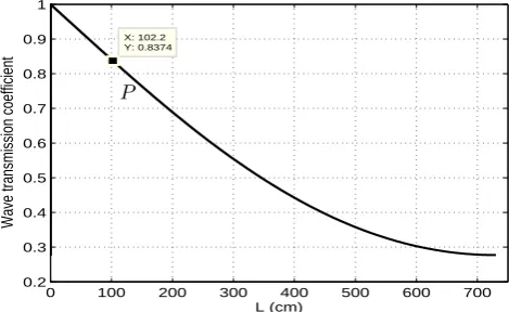
Consider a mangrove belt as a three-layer porous medium with upper, middle and lower layers corresponding to leaves, trunks and roots of mangrove. We propose an approximate model for wave evolution in mangrove as Eq. (21). As a wave breaker, our main concern is the amount of wave energy ab-sorbed by the breakwater. Since wave energy is proportional to the square of wave amplitude, we concern ourselves with the amount of amplitude reduction in a porous belt. Wave transmission coefficientKT is a quantity defined as a ratio between transmitted wave and incident wave amplitudes. If the surface profile in a mangrove belt as a solution of Eq. (21) is known, then theKT curve is just the normalized displace-ment of wave entering the porous medium with zero phase.
An experimental study in Susilo and Ridd (2005) re-ported hydraulic conductivity for mangrove (Rhizophora sp.) as about 10 m day−1 or approximately 0.01 cm s−1. Here, we solve Eq. (21) for three-layer mangrove of equal thickness, with conductivityK1=0.01 cm s−1,K2=
0.03 cm s−1, K3=0.02 cm s−1, and ε=µ2=0.3. We
im-pose a monochromatic wave with period 10 s, or frequency ω=2π/10 rad s−1. The resulting wave transmission coeffi-cient is given in Fig. 4. Note that the curve is plotted with respect to the physical coordinatex¯=Lx=(h¯3/
√
ε)x. In physical dimension, a pointP in Fig. 4 means the follow-ing. For water depthh¯3and the incident wave amplitudea
that satisfiesa/h¯3=ε=0.3, after passing a porous medium
with lengthx¯=102.2 cm, the wave transmission coefficient is 0.8374, which corresponds to an amplitude reduction of
≈16 %.
For a mangrove forest with certain hydraulic conductiv-ity, the wave transmission curveKT clearly depends on the choice of ε(=µ2), and on wave frequencyω. Further, we perform calculations using mangrove conductivity as above, usingε=0.2−0.6 for several wave frequencies, and the re-sults are given in Table 1. For mild wind waves with typical frequency 2π/6 rad s−1, a porous belt length 100 cm gives
0 100 200 300 400 500 600 700
0.2 0.3 0.4 0.5 0.6 0.7 0.8 0.9 1
X: 102.2 Y: 0.8374
L (cm)
Wave transmission coefficient
P
Fig. 4.Wave transmission coefficient curve from numerical computation usingε=µ2= 0.3.
For a mangrove forest with certain hydraulic conductivity, the wave transmission curveKTclearly
depends on the choice ofε(=µ2), and on wave frequencyω. Further, we perform calculations using
235
mangrove conductivity as above, usingε= 0.2−0.6for several wave frequencies and the result are
given in Table 1. For mild wind waves with typical frequency2π/6rad/sec, a porous belt length 100
cm gives wave transmission coefficient0.74to0.82. We note that the recommendation table above
holds for Boussinesq waves, i.e. small amplitude long waves, and the water depth is assumed to be
constant. Moreover, reflection from the beach has been neglected. 240
6 Reflection of a solitary wave
In coastal engineering context it is important to determine how much of the energy of an incoming
‘soliton’ is absorbed by a breakwater, here the three layer porous media. With this in mind we
examine the impact of a soliton propagating across the ocean (depthh3) on a finite length porous
medium of the above type. The soliton is assumed to impact normally on the medium. Of particular 245
interest is the dependence of the transmission coefficientKT on the lengthLof the porous medium
with certain conductivities. The impacting wave is assumed to be long and of small amplitude so
that the standard Boussinesq approximating equations
¯
h3η¯t¯=− (
(¯h3+ ¯η)¯q )
¯
x (32)
¯
q¯t− 1 3 ¯
h23q¯x¯x¯t¯=−
1 ¯
h3
¯
qq¯x¯−g¯h3η¯x¯. (33)
250
are used in the free water zone, see Whitham (1973). These equations are governing equations for
bi-directional gravity waves written in variables surface elevationη¯and horizontal momentumq¯. In
the porous domain, we implement the three-layer Boussinesq equations (21,25) in physical variables,
they read
¯
ηt¯−A¯η¯x¯¯x¯t=K1 (
¯
η¯x( ¯B+R31η¯) )
¯
x (34)
255
Fig. 4. Wave transmission coefficient curve from numerical compu-tation usingε=µ2=0.3.
Table 1. Wave transmission coefficient calculated using conductiv-ity K1=0.01 cm s−1,K2=0.03 cm s−1, and K3=0.02 cm s−1
forε=µ2=0.2−0.6.
Wave freq. Length of mangrove belt
( rad s−1) 100 cm 200 cm 300 cm
2π/16 (swell) 0.86–0.90 0.73–0.81 0.62–0.72 2π/10 0.80–0.86 0.62–0.74 0.46–0.62 2π/6 (mild wind) 0.74–0.82 0.50–0.65 0.32–0.50
wave transmission coefficient 0.74–0.82. We note that the recommendation table above holds for Boussinesq waves, i.e. small-amplitude long waves, and the water depth is assumed to be constant. Moreover, reflection from the beach has been neglected.
6 Reflection of a solitary wave
In a coastal engineering context it is important to determine how much of the energy of an incoming “soliton” is ab-sorbed by a breakwater, here the three-layer porous media.
1028 S. R. Pudjaprasetya: Three-layer porous breakwater
With this in mind, we examine the impact of a soliton prop-agating across the ocean (depthh3) on a finite-length porous
medium of the above type. The soliton is assumed to impact normally on the medium. Of particular interest is the depen-dence of the transmission coefficientKT on the lengthLof the porous medium with certain conductivities. The impact-ing wave is assumed to be long and of small amplitude such that the standard Boussinesq approximating equations
¯
h3η¯t¯= − (h¯3+ ¯η)q¯
¯
x (32)
¯
qt¯− 1 3
¯
h23q¯x¯x¯t¯= − 1
¯
h3 ¯
qq¯x¯−gh¯3η¯x¯. (33) are used in the free-water zone; see Whitham (1973). These equations are governing equations for bi-directional gravity waves written as variables surface elevationη¯and horizontal momentumq. In the porous domain, we implement the three-¯
layer Boussinesq Eqs. (21) and (25) in physical variables; they read
¯
ηt¯− ¯Aη¯x¯x¯t¯=K1 η¯x¯(B¯+R31η)¯
¯
x (34)
¯
Q− ¯CQ¯x¯x¯= −(B¯+ ¯η)η¯x¯, (35) with physical parametersA¯≡ ¯h23A,B¯≡ ¯h3B,C¯≡ ¯h23C. We
simulate a solitary wave initially located upstream of the emerged porous medium. As time progresses, the wave prop-agates through the porous medium and further generates re-flected and transmitted waves. Here we show that the numer-ical predictor–corrector method as explained in Sect. 4 fol-lows through and can be used for solitary wave simulation.
The predictor–corrector method for Boussinesq equations in free areas (32, 33) is described below. We first rewrite Eq. (33) as
ψt¯= − 1
¯
h3 ¯
qq¯x¯−gh3η¯x¯, with ψ= ¯q− 1 3
¯
h23q¯x¯x¯. (36) The new variableψintroduced here is just for computational needs. Its values at grid points relate toq¯ values through a linear correspondence analogous to Eq. (30). The first step implements forward time forward space in Eqs. (32) and (36) for calculating predicted values, indicated by overlines, as follows:
¯
ηnj+1=η¯jn−4t 4x
1
¯
h3
n
(h¯3+ ¯ηjn)(q¯ n j+1− ¯q
n j)+ ¯q
n j(η¯
n j+1− ¯η
n j)
o
9jn+1=9jn+4t 4x
−1
¯
h3
¯
qjn(q¯jn+1− ¯qjn)−gh3η¯jn+1− ¯ηnj
.
The correction step is then
¯
ηnj+1= ¯ηnj
−4t
2h¯3
n
(h¯3+ ¯η)q¯x¯|nj+ ¯qη¯x¯|nj+(h¯3+ ¯η)q¯x¯|jn+1+ ¯qη¯x¯|nj+1 o
9jn+1=9jn
−4t
2
1
¯
h3q¯q¯x¯|
n
j+gh3η¯x¯|nj+
1
¯
h3q¯q¯x¯|
n+1
j +gh3η¯x¯| n+1
j
,
¯
x x¯
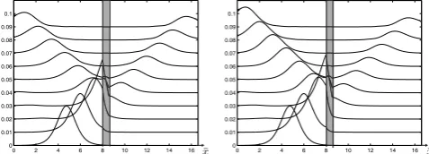
Fig. 5.Surface elevationη¯(¯x,¯t)at subsequent timest0= 0< t1<···< t10= 7sec. Every following curve
is shifted upwards to give 3-dimensional impression. Left:K1= 0.95,K2= 1,K3= 0.95cm/sec, right:
K1= 0.7,K2= 0.75,K3= 0.7cm/sec. All three layers are of the same thicknesses.
LengthLof porous belt
20 cm 30 cm 40 cm 50 cm 60 cm
0.45-0.50 0.40-0.45 0.27-0.33 0.22-0.28 0.20-0.26
Table 2. Wave transmission coefficient for several length of porous medium, calculated using conductivity K1= 0.7,K2= 0.75,K3= 0.7cm/sec fora/h¯3= 0.1−0.4.
Here we show how the solitary wave evolves when it passes an emerged porous medium. The
initial solitary wave profile of Boussinesq with amplitudeais as follows
¯
η(¯x,0) =asech2
{(3a
4¯h3 3
)1/2 (¯x−¯x0)
}
, (43)
¯ q(¯x,0) = g
¯ h33/2 ¯ h3+ ¯η(¯x,0)
¯
η(¯x,0), (44)
290
which travels undisturbed in shape in free water region. Figure 5 presents simulation of an incoming solitary wave with amplitudea= 3cm on a water depth¯h3= 30cm passing through a porous
medium (indicated in grey) with lengthL= 60cm. As the soliton passes through the porous media,
reflected and transmitted waves occur. Amplitude ratio between these two waves depends on the
precise detail of the emerged porous medium, i.e. its lengthLand its hydraulic conductivityKi,i=
295
1,2,3. Smaller conductivity yields smaller amplitude of transmitted wave. For fixed conductivities,
wave transmission coefficient are calculated for several length of porous medium, and the results are
given in Table 2.
12
Fig. 5. Surface elevation η(¯ x,¯ t )¯ at subsequent times t
0=0<
t1< . . . < t10=7 s. Every following curve is shifted upwards
to give a 3-dimensional impression. Left: K1=0.95, K2=1,
K3= 0.95 cm s−1, right:K1=0.7,K2=0.75,K3= 0.7 cm s−1. All
three layers are of the same thicknesses.
Table 2. Wave transmission coefficient for several lengths of porous medium, calculated using conductivity K1=0.7, K2= 0.75 and
K3= 0.7 cm s−1fora/h¯3=0.1−0.4.
LengthLof porous belt
20 cm 30 cm 40 cm 50 cm 60 cm
0.45–0.50 0.40–0.45 0.27–0.33 0.22–0.28 0.20–0.26
where we use forward space to computeq¯x¯|nj,η¯x¯|njand back-ward space to computeq¯x¯|nj+1,η¯x¯|nj+1.
Consider a computational domain with a porous domain in the middle, located on[0, L]. The approximate Eqs. (32) and (33), and the approximate of three-layer model Eqs. (21),(25) are combined. Vertical matching conditions come from the continuity of surface elevation
¯
η|−= ¯η|+, (37)
where−and + denote the left-hand side and the right-hand side of the interface, respectively. In physical variables con-tinuity of horizontal momentum is as follows:
¯
q|0−=K1Q¯|0+, q¯|L+=K1Q¯|L−, (38)
where the termK1Q¯ denotes the reduced horizontal
momen-tum in porous media. These matching conditions are com-monly used for simulations of wave structure interaction, such as in Liu and Wen (1997), Lynett et.al. (2000), Scar-latos and Singh (1987), and Wang and Li (2002).
Here we show how the solitary wave evolves when it passes an emerged porous medium. The initial solitary wave profile of Boussinesq with amplitudeais as follows:
¯
η(x,¯ 0)=asech2 3a 4h¯33
!1/2
(x¯− ¯x0) , (39)
¯
q(x,¯ 0)= g ¯
h33/2
¯
h3+ ¯η(x,¯ 0) ¯
η(x,¯ 0), (40)
which travels undisturbed in shape in free-water regions. Fig-ure 5 presents simulation of an incoming solitary wave with
S. R. Pudjaprasetya: Three-layer porous breakwater 1029
amplitude a=3 cm on a water depth h¯
3=30 cm passing
through a porous medium (indicated in grey) with lengthL=
60 cm. As the soliton passes through the porous medium, reflected and transmitted waves occur. Amplitude ratio be-tween these two waves depends on the precise detail of the emerged porous medium, i.e. its length L and its hy-draulic conductivity Ki, i=1,2,3. Smaller conductivity yields smaller amplitude of transmitted wave. For fixed con-ductivities, wave transmission coefficients are calculated for several lengths of porous medium, and the results are given in Table 2.
7 Conclusions
A non-linear, diffusive and dispersive Boussinesq equation has been derived for surface wave propagation in three-layer porous media. The equation reduces to the Boussinesq equa-tion for one-layer porous media recorded in the literature. The predictor–corrector MacCormack method is a condition-ally stable method for solving the three-layer Boussinesq equations. Numerical simulations of waves propagating into a three-layer system behave like waves propagating into a one-layer system, including the nonlinear effect: the rising of water level at the right end of porous breakwater. The engineering aspect of mangrove in reducing wave energy was considered here from the wave transmission coefficient curve, calculated for a porous belt with typical hydraulic conductivity of mangrove. Further, the MacCormack method was shown to be a stable numerical method for Boussinesq solitary waves. Simulation of reflected and transmitted waves as a result of an initial soliton passing through a three-layer porous medium was performed.
Appendix A
Appendix
Here we give a step-by-step derivation of the Boussinesq Eq. (21) from the full governing equations using the asymp-totic expansion method. We start by solving the normalized Eqs. (13)–(20) layer by layer. Expand each potential8i as a series inµ2:
8i(x, z, t )=8i0+µ28i1+µ48i2+ · · · for i=1,2,3. (A1) The first-order term810is a solution of the order-one term of
the Laplace Eq. (13) with boundary condition (14); it reads 810(x, z, t )=η(x, t ). The first-order terms of interface
con-dition (19) yield8i0(x, z, t )=η(x, t )for i=2,3. Further,
we consider terms ofO(µ2)in equations for the upper-layer (13)–(15); those are
811zz+810xx=0 in 1 (A2)
ηt−εη2x
+811z=0 on z=εη (A3)
811=0 on z=εη. (A4)
Solving Eq. (A2) with810=ηand using the boundary
con-ditions (A3) and (A4) yields
811= −
1
2ηxx(z−εη)
2+εη2 x−ηt
(z−εη). (A5) Next, the orderO(µ2)of (16) is
821zz+820xx=0 in 2. (A6)
Solving the equation above with820=ηand interface con-ditions (19) and (20) with811as given in Eq. (A5) yields
821= −
1 2ηxx
n
(z+h1)2+(h1+εη)2
o
−εη2x−ηt
(h1+εη)
+R12
n
ηxx(h1+εη)+εηx2−ηt
o
(z+h1), (A7)
withRij=Ki/Kj fori, j=1,2,3. Next, theO(µ2)terms in equations for the third-layer (17) and (18) are
831zz+830xx=0 in 3 (A8)
831z=0 on z= −h3 (A9)
Solving Eq. (A8) with830=ηand boundary condition (A9) and interface conditions (19) for z= −h2 with 821 as in
Eq. (A7) yields 831= −
1 2ηxx
n
(z+h3)2−(h3−h2)2+(h2−h1)2+(h1+εη)2 o
+R12
n
ηxx(h1+εη)+εηx2−ηt
o
(h1−h2)
−εη2x−ηt/K1
(h1+εη). (A10)
To get an approximate evolution equation of the orderO(µ2) from the interface condition alongz= −h2, we still need to
calculate the order-one term of822zand832z. Higher-order calculation is made under the assumptionε=µ2, and fol-lowed by collecting theO(µ4)terms. The equations for the first layer are
812zz+811xx=0 in 1 (A11)
−810xηx+812z=0 on z=εη. (A12) Solving Eq. (A11) with the boundary conditions (A12) yields 812z=
1
6η4x(z−εη)
3+ 1
2K1
ηtxx(z−εη)2
+η2x+O(µ2). (A13)
Next,822zcan be obtained from theO(µ4)term in the equa-tion for the second layer
1030 S. R. Pudjaprasetya: Three-layer porous breakwater
with the boundary condition (20) forz= −h1, and we get
822z= 1
6η4x(z+h1)
3+
1
2η4xh
2
1−h1ηtxx
(z+h1)
−R12{η4xh1−ηtxx}
1
2(z+h1)
2
+R12
−1
6η4xh
3 1+
1 2h
2
1ηtxx+η2x
+O(µ2). (A15) Next, collecting theO(µ4)terms in the equations for the third layer, we get
832zz+831xx=0 in 3 (A16)
832z=0 on z= −h3. (A17)
Solving Eq. (A16) with boundary conditions (A17) yields 832z=
1
6η4x(z+h3)
3
+1
2η4x
n
−(h3−h2)2+(h2−h1)2+h21
o
(z+h3)
− {R12(η4xh1−ηtxx) (h1−h2)+h1ηtxx}(z+h3)
+O(µ2). (A18)
Substituting Eqs. (A7), (A10) and (A15), (A18) into the in-terface condition (20) alongz= −h2 yields the following
equation:
ηt−µ2Aηxxt=(ηx(B+εR31η))x, (A19) with A and B given in Eqs. (23) and (22), respectively. Hence, the approximate Boussinesq Eq. (A19) has been de-rived.
Acknowledgements. We thank the reviewers for their thorough
review, which significantly contributed to improving the quality of the manuscript. Some discussions at the early stage of this study with L. H. Wiryanto, A. Y. Gunawan, Lina, Viska, and Antonius are also acknowledged. Financial support from Riset KK ITB, No. 242/I.1.C01/PL/2013 and partly from Riset Desentralisasi ITB 2013 are appreciated.
Edited by: R. Grimshaw
Reviewed by: S. N. Bora, N. Fowkes, and one anonymous referee
References
Chwang, A. T. and Chan, A. T.: Interaction between porous media and wave motion, Annu. Rev. Fluid Mech., 30, 53–84, 1998. Dahdouh-Guebas, F.: Mangrove forests and tsunami
protec-tion, 2006 McGraw-Hill Yearbook of Science & Technology, McGraw-Hill Professional, New York, USA, 187–191, 2006. Fernando, H. J. S., Samarawickrama, S. P., Balasubramanian, S.,
Hettiarachchi, S. S. L., and Voropayev, S.: Effects of porous bar-riers such as coral reefs on coastal wave propagation, Journal of Hydro-environment Research, 1, 187–194, 2008.
Kathiresan, K. and Rajendran, N.: Comments on “Coastal man-grove forests mitigated tsunami”, Estuar Coast. Shelf S., 67, 539– 541, 2006.
Lynett, P. J., Liu, P. L. F., Losada, I. J., and Vidal, C.: Solitary wave interaction with porous breakwaters, J. Waterw. Port C.-ASCE, 314–322, 2000.
Madsen, O. S.: Wave transmission through porous structures, J. Wa-terway Div.-ASCE, 100, 169–188, 1974.
Masda, Y., Magi, M., Kogo, M., and Nguyen Hong, P.: Mangrove as a coastal protection from waves in the Tong King delta, Vietnam, Mangroves and Salt Marshes, 1, 127–135, 1997.
Massel, S. R., Furukawa, K., and Brinkman, R. M.: Surface wave propagation in mangrove forests, Fluid Dyn. Res., 24, 219–249, 1999.
Nielsen, P.: Tidal dynamics of the water table in beaches, Water Resour. Res., 26, 2127–2134, 1990.
Lin, P. and Anuja Karunarathna, S. A. S.: Numerical Study of Solitary Wave Interaction with Porous Breakwaters, J Wa-terw. Port C.-ASCE, 133, 352–363, doi:10.1061/(ASCE)0733-950X(2007)133:5(352), 2007.
Liu, P. L. F. and Jiangang Wen, J.: Nonlinear diffusive surface waves in porous media, J. Fluid Mech., 347, 119–139, 1997.
Liu, P. L. F., Lin, P., Chang, K. A., and Sakakiyama, T.: Numeri-cal modeling of wave interaction with porous structures, J. Wa-terw. Port C.-ASCE, 125, 322–330, doi:10.1061/(ASCE)0733-950X(1999)125:6(322), 1999.
Liu, W. C., Hsu, M.H., and Wang, C.F.: Modeling of Flow Resistance in Mangrove Swamp at Mouth of Tidal Keelung River, Taiwan, J. Waterw. Port C.-ASCE, 129, 86–92, doi:10.1061/(ASCE)0733-950X(2003)129:2(86), 2003. Scarlatos, P. D. and Singh, V. P.: Long wave transmission through
porous breakwaters, Coast. Eng., 11, 141–157, 1987.
Sollitt, C. K. and Cross, R. H.: Long-wave transmission through porous breakwaters, in: Proc. 13th Coastal Eng. Conf., ASCE, New York, USA, 3, 1827–1846, 1972.
Sulisz, W.: Wave reflection and transmission at permeable breakwa-ters of arbitrary cross-section, Coast. Eng., 9, 371–386, 1985. Susilo, A. and Ridd, P. V.: The bulk hydraulic conductivity of
man-grove soil perforated with animal burrows, Wetl. Ecol. Manag., 13, 123–133, 2005.
Teh, S. Y., Koh, H. L., Liu, P. L. F., Ismail, A. I. Md., and Lee, H. L.: Analytical and numerical simulation of tsunami mitigation by mangroves in Penang, Malaysia, J. Asian Earth Sci., 36, 38– 46, 2009.
van Gent, M. R. A.: Wave interaction with permeable coastal struc-ture, Ph.D. thesis, Delft University, Delft, the Netherlands, 1995. Vo-Luong, H. P. and Massel, S.: Energy dissipation in non-uniform mangrove forests of arbitrary depth, J. Marine Syst., 74, 603– 662, 2008.
Wang, K. H. and Li, W.: Modeling propagation of nonlinear shallow-water waves past a porous barrier, in: Proc. 15th Eng. Mech. Div. Conf. of the American Soc. of Civil Engineers, Columbia University, New York, USA, 2–5 June 2002.
Whitham, G. B.: Linear and Nonlinear Waves, John Wiley & Sons, Inc., New York, USA, 1973.