www.clim-past.net/10/269/2014/ doi:10.5194/cp-10-269-2014
© Author(s) 2014. CC Attribution 3.0 License.
Climate
of the Past
Modeling Northern Hemisphere ice-sheet distribution during MIS 5
and MIS 7 glacial inceptions
F. Colleoni1, S. Masina1,2, A. Cherchi1,2, A. Navarra1,2, C. Ritz3, V. Peyaud3, and B. Otto-Bliesner4 1Centro Euro-Mediterraneo sui Cambiamenti Climatici, Bologna, Italy
2Istituto Nazionale di Geofisica e di Vulcanologia, Bologna, Italy
3CNRS/Université Joseph Fourier, Grenoble 1, LGGE, St Martin d’Hères cedex, France
4Climate and Global Dynamics Division, National Center for Atmospheric Research, Boulder, CO, USA Correspondence to: F. Colleoni (flocolleoni@gmail.com)
Received: 14 November 2012 – Published in Clim. Past Discuss.: 18 December 2012 Revised: 12 December 2013 – Accepted: 7 January 2014 – Published: 7 February 2014
Abstract. The present manuscript compares Marine
Iso-tope Stage 5 (MIS 5, 125–115 kyr BP) and MIS 7 (236– 229 kyr BP) with the aim to investigate the origin of the difference in ice-sheet growth over the Northern Hemi-sphere high latitudes between these last two inceptions. Our approach combines a low resolution coupled atmosphere– ocean–sea-ice general circulation model and a 3-D thermo-mechanical ice-sheet model to simulate the state of the ice sheets associated with the inception climate states of MIS 5 and MIS 7. Our results show that external forcing (orbitals and GHG) and sea-ice albedo feedbacks are the main fac-tors responsible for the difference in the land-ice initial state between MIS 5 and MIS 7 and that our cold climate model bias impacts more during a cold inception, such as MIS 7, than during a warm inception, such as MIS 5. In addition, if proper ice-elevation and albedo feedbacks are not taken into consideration, the evolution towards glacial inception is hardly simulated, especially for MIS 7. Finally, results high-light that while simulated ice volumes for MIS 5 glacial in-ception almost fit with paleo-reconstructions, the lack of pre-cipitation over high latitudes, identified as a bias of our cli-mate model, does not allow for a proper simulation of MIS 7 glacial inception.
1 Introduction
Glacial inceptions represent a transition from a warm to a cold mean climate state (Calov et al., 2005b). Indeed, considering the sea-level records during these warm-to-cold
transitions, Northern Hemisphere ice sheets were only lit-tle developed over North America and Eurasia compared to the glacial maxima (Fig. 1d). Concerns about the capabil-ity of climate models to properly simulate future climates have emerged from the large uncertainties and lack of flexi-bility of the same models to simulate past climate transitions from warm to cold conditions (Calov et al., 2005b). There-fore, glacial inceptions are an interesting phenomenon with which to test the capability of models to simulate climates slightly warmer or slightly colder than present-day climate.
It is now accepted that Northern Hemisphere ice sheets started to develop only if both insolation and greenhouse gases (GHGs) dropped significantly (e.g., Berger, 1978; Bonelli et al., 2009). The amplitude of the drop in inso-lation and GHGs, however, differs between each glacial inceptions. During the last two glacial inceptions, namely MIS 5 (≈125–115 kyr BP) and MIS 7 (≈236–229 kyr BP), the concentration of atmospheric CO2 retrieved from East
Antarctica (Luthi et al., 2008) peaked to a rather simi-lar value, but dropped by a simi-larger amount during MIS 7 glacial inception (Fig. 1f). After≈242 kyr BP, CO2dropped
well below 260 ppm, while after 125 kyr BP, CO2remained
above 260 ppm until≈110 kyr BP. Similarly, the largest drop in atmospheric CH4 concentration occurs after 242 kyr BP
0 100 200 300 Time (kyrs BP)
−8 −4 0 4 Antarctic Δ T (°C) 180 200 220 240 260 280 CO2 (ppmv) 400 500 600 700 CH4 (ppbv) −120 −80 −40 0
Sea level (m)
−120 −80 −40 0 −0.50.0 0.5 1.0 −0.50.0 0.5 1.0 Benthic δ 13C (‰) 440 480 520 560 JJA inso.(W.m 2) 440 480 520 560 −0.05 0.00 0.05 e*sin( ω ) 22 23 24 Obl. (°)
0 100 200 TIII 300
TIII TII TII a. b. c. d. e. f. g. MIS5 MIS7 NADW AABW 70°S 65°N
Fig. 1. Overview of the two last glacial cycles illustrated by different forcing and proxies. From top to bottom: (a) obliquity (◦) and precession index (Laskar et al., 2004); (b) summer insolation at 65◦N and 70◦S (W m−2Laskar et al., 2004); (c) benthicδ13C indicative of the changes in sources of the North Atlantic deep waters formation at the Mediterranean latitudes (Martrat et al., 2007); (d) sea-level reconstructions (m) from Waelbroeck et al. (2002); (e) atmospheric CH4(ppbv Loulergue et al., 2008) concentrations from EPICA Dome C, East Antarctica; (f) CO2(ppmv Luthi et al., 2008) concentrations from EPICA Dome C, East Antarctica; (g) temperature anomaly (◦C) relatively to present day (Jouzel et al., 2007), retrieved from deuterium excess, EPICA Dome C, East Antarctica. Vertical grey bars indicate the time of the climate snapshots simulations performed in this work. Termination II (TII) and Termination III (TIII) are indicated as well.
An additional remarkable difference between the last two glacial inceptions is the state of the continental ice volume at the beginning of each glacial inception. While the maxi-mum sea-level fall was similar between the last two glacial cycles, the maximum sea-level rise during the last two in-terglacials varied with estimates above or below present-day sea level (Fig. 1d, Rabineau et al., 2006; Caputo, 2007). In fact, for the last interglacial (≈125 kyr BP), proxies indicate a sea-level rise between 4 to 10 m a.m.s.l. (above mean sea level, Stirling et al., 1995; Kopp et al., 2009; McCulloch and Esat, 2000) implying that part of present-day Antarc-tica and Greenland ice sheets melted out. In contrast, Dutton et al. (2009) suggest that during the penultimate interglacial,
≈245 kyr BP, sea level never rose above present-day mean sea level.
Because of those GHGs particularities (low values during MIS 7) and of the difference in sea level between MIS 5 and MIS 7, we focus our investigations on the Northern Hemi-sphere ice-sheet distribution of MIS 5 (≈125–116 kyr BP) and MIS 7 (≈236–229 kyr BP) glacial inceptions. More specifically we investigate the impact of orbital parame-ters and GHGs on the growth of ice sheets in the Northern
Hemisphere high latitudes. We use an earth system model (in its fully coupled AOGCM version) with appropriate GHGs and orbital forcing to simulate the climate of the inceptions under investigation. The climate simulated by the coupled model is then used to force off-line a 3-D thermo-mechanical ice-sheet model.
simulated a sea-level drop by estimating the amount of peren-nial snow accumulated over the Northern Hemisphere high latitudes using steady-state experiments (e.g., Vettoretti and Peltier, 2003; Jochum et al., 2011) or transient experiments (e.g., Wang and Mysak, 2002). In these studies the mod-els used were able to broadly simulate perennial snow and ice-sheet growth in the Northern Hemisphere high latitudes where geological evidence is indicative of glacial inception areas. Other studies have performed idealized experiments to determine the thresholds of various regional feedbacks in the climate system that could have triggered a glacial incep-tion in the Northern Hemisphere high latitudes (e.g., Calov et al., 2005a, b). Some of the modeling studies have shown the importance of vegetation and dust in amplifying or in-hibiting the growth of the ice sheets during the last two glacial cycles (e.g., de Noblet et al., 1996; Vettoretti and Peltier, 2004; Kageyama et al., 2004; Calov et al., 2005a; Krinner et al., 2006; Colleoni et al., 2009b, a). For exam-ple, Kubatzki et al. (2006), using a fully coupled climate– ice-sheet EMIC, showed that during the last glacial inception (≈113 kyr BP in their study) the growth of the Laurentide ice sheet could have been delayed by modulating the state of ocean and vegetation. In the same line, Born et al. (2010) suggest that, during the last glacial inception (≈115 kyr BP), the growth of the Eurasian ice sheet was delayed by a persis-tent high oceanic heat transport towards the Northern Hemi-sphere high-latitude regions.
The present work differs from the previous studies afore-mentioned for two reasons. The first deals with the treat-ment of the marine margins in the ISM. In the recent work of Herrington and Poulsen (2012) about the last glacial in-ception (≈115 kyr BP) over North America, no explicit ice shelves are simulated, but their ISM allows for floating ice over areas where ocean depth does not exceed 750 m. The limitation of this method resides in the fact that it may partly limit the growth of ice over oceanic regions deeper than 750 meters and as a consequence may induce incorrect ice dis-tribution and volume. It is worth noting that in our ISM, ice shelves are explicitly simulated but a melting rate of 2.45 m yr−1is prescribed below the shelves for ocean depths larger than 450 m. Born et al. (2010) focused on the entire Northern Hemisphere but no ice shelf dynamics was consid-ered. They argued that given the low ice volume observed during the last inception, the treatment of the marine part was of minor importance. Contrary to these this study, Peyaud et al. (2007) showed that the floating part of the Eurasian ice sheet was essential to its rapid multiple advances and retreats during the last glacial cycle. Even if at the time of the last glacial inception, ice volume was low over both North Amer-ica and Eurasia, this might not have been the case during MIS 7 glacial inception. For this reason, in the present study, we account for ice shelf dynamics in our ISM simulations.
The second reason deals with the initial conditions in the ISM. Most of past studies have modeled climate and ice sheets of the last glacial inception towards 115 kyr BP,
or for the entire last glacial cycle but discarding the peak interglacial of MIS 5. At that time, Eurasia and North Amer-ica were ice free and the amount of ice that survived over Greenland is still uncertain. This is why most of the past modeling studies choose to initialize MIS 5 climate either with present-day ice cover or with no ice over Greenland. Contrary to MIS 5, MIS 7 recorded a sea level lower than present day. This implies that some continental ice may have survived from the previous glacial cycle over Eurasia and North America or that the Greenland ice sheet was larger than today, or both. Therefore, we choose to spin up the ini-tial ISM topography to simulated pre-inception climates (i.e., with orbital configuration not favorable to glaciation) in or-der to obtain an initial Northern Hemisphere ice-sheet topog-raphy more in agreement with the time periods considered in our work. Nonetheless, the aim of this study is not to recon-struct a realistic ice evolution over the Northern Hemisphere, but to investigate the main differences resulting from differ-ent external forcing. Therefore, the evolution of Greenland in our study is only indicative.
The manuscript is structured as follows: Sect. 2 describes the coupled model, the ice-sheet model, the experimental setup as well as the forcing method used for the ISM sim-ulations; Sect. 3 shows the results from the climate and the ISM models simulations; Sect. 4 discusses the main results in terms of hypothesis at the base of the work. Section 5 sum-marizes the main conclusions.
2 Methods
We force a 3-D thermo-mechanical ice-sheet model off-line with climate states obtained from atmosphere–ocean coupled simulations. To account for the time evolution of the feed-backs that we want to investigate, we modulate the climate forcing in our ISM experiments by means of a temperature index retrieved from Greenland ice cores. This method has been already used in several studies focusing on specific time slices of the last glacial cycle and has provided realistic re-sults of the ice-sheet evolution over North America and Eura-sia (Peyaud et al., 2007; Charbit et al., 2007), over Greenland (Letréguilly et al., 1991; Greve, 2005; Quiquet et al., 2013) and over the Tibetan Plateau (Kirchner et al., 2011).
2.1 Community Earth System Model (CESM)
Table 1. Climate experiments settings. Greenhouse gas concentrations were retrieved from EPICA Dome C, East Antarctica and come from Luthi et al. (2008) for the CO2, Loulergue et al. (2008) for the CH4and Schilt et al. (2010) for the NO2records. The orbital parameters for the pre-industrial control experiment (CTR1850) were set to 1990 while the greenhouse gas were set at their pre-industrial values. For K115 and K229 experiments, the runs were initialized at the 400th model year of the K125 and K236 experiments, respectively.
ID Epoch Perihelion Obliquity CO2 CH4 NO2 Spin-up Length
date (◦) (ppm) (ppb) (ppb) (model
years)
CTR0K 1990 4 Jan 23.44 367 1760 316 Present day 400
CTR1850 1990 4 Jan 23.44 284 791 275 Pre-ind. 700
K115 115 kyr BP 14 Jan 22.44 262 472 251 K125 branch 300
K125 125 kyr BP 23 Jul 23.86 276 640 263 125 k 700
K229 229 kyr BP 3 Feb 22.22 224 493 256 K236 branch 300
K236 236 kyr BP 2 Oct 22.34 241 481 267 236 k 700
vegetation and dynamical aeolian dust distribution, but we turned off those options, prescribing the pre-industrial veg-etation cover and dust distribution over continents in all our experiments since in this work we want to focus on the im-pact of external forcing.
CESM experiments setup
The two glacial inceptions under investigation have been se-lected using the values of the proxy records displayed in Fig. 1. The four snapshots referring to the inception periods are identified by the vertical blue boxes. For the last glacial cycle, the timing of inception is commonly defined in liter-ature between 116–113 kyr BP. In this study, we set up the inception simulations with 115 kyr BP orbital and GHGs val-ues. Determining the timing of the penultimate inception was harder, as observed on the sea-level records (Fig. 1d), since the penultimate glacial cycle does not exhibit a regular de-creasing trend in sea level as for the last glacial cycle. This period is characterized by three sea-level high-stands (even if below present-day sea level), the first one occurring right after Termination III towards≈231 kyr BP, the second one occurring towards≈206 kyr BP and the last one occurring toward ≈189 kyr BP (Dutton et al., 2009). Considering the sea-level evolution, the penultimate inception occurred af-ter 189 kyr BP. On the other hand, considering GHGs and Antarctica temperature anomaly, the largest peaks occurred right after Termination III, setting the beginning of a new cycle towards 240 kyr BP (Fig. 1e and f). Taking the peak GHGs as a reference state for the beginning of the new cy-cle, we selected the penultimate inception period using the epoch of the nearest orbital state presenting characteristics similar with the inception at 115 kyr BP. The simulation was consequently set up with 229 kyr BP orbitals and GHGs val-ues. Masson-Delmotte et al. (2010) show that in East Antarc-tica ice core records, the climate evolution before those two glacial inceptions was highly different. In their work, the last interglacial (≈130 kyr BP) appears to be the warmest of the last 800 kyr and was preceded by one of the mildest glacial
periods on record, characterized by a moderate sea-level drop similar to that occurred at the Last Glacial Maximum (LGM). In contrast, the penultimate interglacial (≈245 kyr BP) was cool and was preceded by one of the coldest glacial peri-ods on record, characterized by a large drop in sea level. To account for this difference in our ISM experiments, we set up two additional simulations with orbital and GHGs val-ues defined as a compromise between the time of maximum Northern high latitudes summer insolation and the time of the highest sea level preceding each glacial inception (Fig. 1d): one at 125 kyr BP and one at 236 kyr BP.
In summary, six experiments, different in orbital param-eters and atmospheric greenhouse gas concentrations, were carried out to explore the discrepancies between MIS 5 and MIS 7 glacial inceptions: a present-day run (CTR0k) ac-counting for present-day GHGs values, used to show CESM performances; a control run resulting from natural variabil-ity only, set to pre-industrial initial conditions (CTR1850) to be compared with our paleo-simulations; two MIS 5 ex-periments set at 125 kyr BP (K125) and 115 kyr BP (K115) and two MIS 7 experiments set at 236 kyr BP (K236) and 229 kyr BP (K229) (see Table 1). The two inceptions experi-ments, namely K115 and K229, were branched from K125 and K236, respectively, after 400 years of simulation and were then continued for 700 yr. However, to compare the same model years with the branch experiments, CTR1850, K125 and K236 were also continued to 700 model years. A slight drift still persists in the experiments due to the abyssal circulation (not shown). However, we assume that this drift is small enough to not affect our main conclusions.
2.2 GRenoble Ice Shelf and Land Ice model (GRISLI)
approximation (Hutter, 1983, SIA), whereas ice shelves and ice streams are simulated following the shallow shelf approx-imation (MacAyeal, 1989, SSA). For more details about the physics, the reader may refer to Rommelaere and Ritz (1996) and Ritz et al. (2001). The ice shelf formulation in GRISLI allows for a more realistic calculation of the ice-sheet growth, and particularly of the advance of ice onto the shallow con-tinental shelves in both hemispheres high latitudes during glaciations. GRISLI is thus particularly adapted for simu-lating past ice-sheet evolution over time (e.g., Álvarez-Solas et al., 2011; Peyaud et al., 2007).
Ice shelf front positions are determined with a scheme where two thickness criteria must be fulfilled: (1) calving occurs at the ice shelf front when the ice thickness is be-low 150 m. This value was set up according to Peyaud et al. (2007) and it corresponds to the thickness of most observed ice shelf fronts; (2) for each grid point at the front, the ice coming from the upstream points must fail to main-tain a thickness above the threshold. Ice shelves geograph-ical distribution is also controlled by basal melting set ac-cording to a depth criterion. Above 450 m depth basal melt-ing is 0.2 m yr−1 while below this depth basal melting is 2.45 m yr−1.
The experiments have been designed on a 40 km reg-ular rectangreg-ular grid from ≈47◦N to the North Pole. Non-uniform geothermal heat fluxes are prescribed after Shapiro and Ritzwoller (2004). Since we do not have any precise information about dimensions of the Green-land ice sheet for the periods we are modeling, we initial-ize our experiments with present-day Greenland ice-sheet topography adapted from ETOPO2 dataset (NOAA, http: //www.ngdc.noaa.gov/mgg/global/etopo2.html). We assume that the residual glacio-isostatic response from the LGM (≈21 kyr BP) is small enough to consider the present-day to-pography to be in isostatic equilibrium. Greenland ice sheet is spun up to pre-inception climates K125 and K236 (see Sect. 2.2.2).
2.2.1 Temperature index
Reconstructing the time-evolution of past climate to force an ice-sheet model is crucial for the outcomes of the simula-tions. Previous studies using GRISLI, have realistically sim-ulated the last deglaciation (Charbit et al., 2007), or the Early Weischelian Eurasian ice-sheet growth (Peyaud et al., 2007), or more recently Greenland ice sheet over the last 130 kyr BP (Quiquet, 2012; Quiquet et al., 2013), using indices to mod-ulate climate forcing. Bonelli et al. (2009) performed tran-sient experiments over the entire last glacial cycle using the coupled CLIMBER–GRISLI model (only grounded ice) and modulating some of the simulated variables by means of an index (aeolian dust deposition for example).
To construct our temperature index, we used two dif-ferent published temperature anomaly reconstructions. The first temperature index 1TGR is the one reconstructed for
Greenland over the last two glacial cycles by Quiquet (2012). This index combines three different types of records: North GRIP δ18O record (central Greenland, North GRIP mem-bers, 2004), North Atlantic ODP 980 sea surface tempera-tures record (Oppo et al., 2006) and EPICA Dome C, CH4
record (East Antarctica, Loulergue et al., 2008). The recon-struction is shown in Fig. 3a and the temperature index is expressed as a temperature anomaly relative to pre-industrial time period. For more details about the method see Quiquet et al. (2013). Since1TGR corresponds to the evolution of
Greenland temperature over time, we assume that this index is consequently broadly representative of the variations in at-mospheric temperature over Northern Hemisphere high lati-tudes in general.
The temperature index 1TGR is based on various types
of observations and results from the feedbacks of the en-tire earth’s climate system. On the contrary, in our climate simulations, we only account for orbitals and GHGs varia-tions. The only simulated ice albedo feedback is due to the sea-ice cover fluctuations. Therefore, the temperature index reconstructed by Quiquet et al. (2013) in its actual shape is not fully consistent with our simulations. To retrieve a time evolution temperature index given by the combination of insolation, GHGs and sea-ice albedo, we considered the reconstructions by Köhler et al. (2010) who used an ideal-ized radiative model applied to various proxy records from Antarctica. Köhler et al. (2010) managed to calculate the mean annual global temperature anomaly, relative to pre-industrial, resulting from the main climate feedbacks acting at paleo-timescale as
1TtotK=1TorbitK +1TGHGK +1Tland cryoK +1Tsea iceK +1TvegK +1TdustK ,(1) where1TorbitK ,1TGHGK ,1Tland cryoK ,1Tsea iceK ,1TvegK,1TdustK , are the contributions from orbitals, GHGs, land-ice albedo, sea-ice albedo, vegetation and dust, respectively. Köhler et al. (2010) show that1TtotK represents half of the signal from the temperature anomaly retrieved from deuterium excess in East Antarctica (Jouzel et al., 2007). Moreover, the temperature anomaly that they calculated is global, and to apply it to our ice-sheet simulations over the Northern Hemisphere high lat-itudes, we would need to estimate the time evolution of polar amplification over the high latitudes. Since we cannot cal-culate it over the time periods considered here, we simply calculated the proportion of total signal (1TtotK) represented by the combination of orbitals (1TorbitK ), GHGs (1TGHGK ) and sea-ice (1Tsea iceK ). We finally multiplied Quiquet (2012) tem-perature index1TGRby this ratio:
1TGIS =1TGR×
1TorbitK +1TGHGK +1Tsea iceK
1TtotK . (2)
The temperature index is displayed for both periods in Fig. 3b and c. For MIS 5,1TGIS increases of about 6◦C at
40 60 80
Latitudes
0 1 2 3 4 5 6 7 8 9 10 11 12
236k − CTR1850 d.
−100 −80 −60 −40 −20 0 20 40 60 80 100
W/m2 40
60 80
Latitudes
229k − CTR1850 b.
40 60 80
Latitudes
125k − CTR1850 c.
40 60 80
Latitudes
0 1 2 3 4 5 6 7 8 9 10 11 12
Months
115k − CTR1850 a.
Fig. 2. Solar downward radiation anomaly at top of the atmo-sphere (W m−2) over the northern high latitudes (40–90◦N) be-tween CTR1850 and the experiments described in Table 1.
of about 7◦C after 122 kyr BP, in agreement with the
evolu-tion of the Greenland temperature index from Quiquet et al. (2013) (Fig. 3a and b). For MIS 7, the temperature index is always negative and the maximum temperature decrease is of 2.5◦C relative to 236 kyr BP value (Fig. 3c). For this period,
1TGISsuggests that the role of combined orbitals, GHGs and
sea-ice to the total signal is minor (Fig. 3a and c).
The temperature index is then used to define a glacial in-dex function:
I|GIS
(t ) =
1T|GIS
(t ) −1T125k,236kGIS
1T115k,229kGIS −1T125k,236kGIS . (3)
Table 2. Ice-sheet experiments settings. The experiments are split into two groups: steady state and transient. The steady-states SS229 and SS115 have been branch from SS236 and SS125 respectively. For the transient experiments T115-GIS and T229-GIS, the climate evolution between [236–229 k] and [125–115 k] is perturbed by a temperature index accounting for insolation, greenhouse gas and sea-ice albedo (IGIS) feedbacks from Köhler et al. (2010).
ID IGIS Climate Length Spin-up
(◦C) (◦C) (kyr)
SS236 K236 0–150
SS229 K229 150–300 SS236
SS125 K125 0–150
SS115 K115 150–300 SS125
T229-GIS X K236–K229 8 SS236
T115-GIS X K125–K115 10 SS125
I|GIS
(t ) is defined such thatI|
GIS
(t ) = 0 for the initial time step and denotes interglacial conditions while I|GIS
(t ) = 1 for the final time step denotes more glacial inception conditions (Fig. 3d and e). Therefore, the function is calculated such that I|GIS
(t ) <0 corresponds to warmer climate conditions while I|GIS
(t ) >0 corresponds to colder climate conditions. The glacial index function for both periods is displayed in Fig. 3d and e. In the following sections, I|GIS
(t ) will be re-ferred to asIGIS. Note that with this index, we do not aim at
reconstructing the exact conditions during MIS 5 and MIS 7 over the Northern Hemisphere. In fact,IGISis idealized and
probably overestimates the Northern Hemisphere contribu-tion of the feedbacks included in their calculacontribu-tion since orig-inal data1TGIS is based on central Greenland temperature
proxies. Nevertheless,IGIS is indicative of the natural trend
of climate evolution in the Northern high latitudes during both time periods.
2.2.2 Ice-sheet experiments setup
Two series of experiments were performed: (1) steady state and (2) transient. To carry out the steady-state experiments, GRISLI was run for 150 000 model years both for 236 kyr BP (SS236) and 125 kyr BP (SS125) time periods using K236 and K125 climate forcing and starting from present-day to-pography. The steady-state runs for 229 kyr BP (SS229) and 115 kyr BP (SS115) were branched from the last iteration of previous steady-state experiments (SS236 and SS125). They were forced using K115 and K125 climates and ran for a fur-ther 150 000 model years (Table 2).
−8 −6 −4 −2 0 2 4
IGIS(t)
116 120 124
Time (kyrs BP) d.
−2 0 2 4
IGIS(t)
228 232 236
Time (kyrs BP) e.
−15 −10 −5 0 5 10
∆
T(°C)
116 120 124
b.
∆ TGIS
∆ TGR
−15 −10 −5 0 5 10
∆
T(°C)
228 232 236
c. −20
−15 −10 −5 0 5 10
∆
TGR
(°C)
0 20 40 60 80 100 120 140 160 180 200 220 240
Time (kyrs BP)
a.
Fig. 3. Temperature indices considered in this work: (a) temperature index1TGR(anomaly relative to pre-industrial in◦C) after Quiquet (2012). (b) and (c)1TGR(black) as in (a) represented by combined contribution of orbitals, GHGs and sea-ice-cover albedo feedbacks (1TGIS) retrieved from Köhler et al. (2010). See Methods for more details on the calculations. Dark blue squares correspond to the simulated mean annual central Greenland temperature anomaly (relative to CTR1850) for each of the CESM experiments (Table 1). The light blue square corresponds to the central Greenland temperature anomaly between pre-industrial and 115 kyr BP simulated climates at 1◦×1◦ horizontal resolution from Jochum et al. (2011). (d) and (e) glacial index function (Equ. 3) used in the ice-sheet experiments,IGISincluding orbitals, GHGs and sea-ice albedo.
where the initial ice topography is that of the steady states for each period, that is, SS236 and SS125, respectively. Since we have available only two simulated climatologies for each inception period, the time evolution of temperature between K236 and K229 and between K125 and K115 is interpolated during the time integrations.
Temperature is corrected for elevation changes,
1Ttopo|(x,y,t ), using a spatially uniform lapse rate of 5◦C km−1for mean winter temperature (Abe-Ouchi et al., 2007; Bonelli et al., 2009) and 4◦C km−1for mean summer temperature (Bonelli et al., 2009). The annual temperature cycle in GRISLI is approximated by a sinusoidal function
based on mean annual and warmest summer month CESM temperatures. Since a simple linear interpolation might not realistically represent the observed time evolution of climate between each simulated climatology (Fig. 1), a time-dependent perturbation is accounted for, following Greve (2005):
1TS2pert−S1|(x,y,t )=I|GIS
(t ) ×1TS2−S1|(x,y) (4)
Trec|(x,y,t ) =TS1|(x,y)+1TS2pert−S1|(x,y,t )+1Ttopo|(x,y,t ),(5)
where 1TS2−S1|(x,y) is the anomaly between our simu-lated climate snapshots (i.e., K115–K125 and K229–K236), and where I|GIS
precipitation field is achieved similarly to temperature, ac-counting forI|GIS
(t ) . Note that the use of exponential function in the precipitation formulation is motivated by the saturation pressure of water vapor in the atmosphere which increases roughly exponentially with temperature:
Prec|(x,y,t ) = PS1|(x,y)×exp
I|GIS
(t ) ×ln
P
S2|(x,y)
PS1|(x,y)
, (6)
where PPS2|(x,y)
S1|(x,y) is the ratio between our simulated climate
snapshots and calculated as K115/K125 and K229/K236. Precipitation is converted into snowfall when air temperature drops below 2◦C. The ablation is calculated using the
pos-itive degree day method (PDD, Reeh, 1991) for which the melting coefficients have been set toCsnow= 3 mm◦C−1d−1
andCice= 8 mm◦C−1d−1. Finally, 60 % of surface melt is
able to refreeze.
Two sets of transient experiments were performed, namely T115-GIS and T229-GIS based on the temperature index ac-counting for orbitals, GHGs and sea-ice albedo variations (Table 2).
3 Results
3.1 CESM climate simulations
The orbitals for both inceptions are almost similar since per-ihelion occurred in mid-January for K115 and at the be-ginning of February for K229 (Table 1). This leads to a similar solar incoming downward radiation pattern over the Northern Hemisphere high latitudes with colder summers and slightly warmer winters with respect to the pre-industrial control run CTR1850 (Fig. 2). In contrast, pre-inception sim-ulations K125 and K236 differ, with perihelion dates in late July and in early October, respectively (Table 1). This has consequences on permanent snow cover, which is likely to disappear in K125 due to the strong summer insolation.
Compared to CTR1850, mean summer air temperature (JJA) for K125 is warmer by about 3◦C over the North-ern Hemisphere high latitudes, while for all the other peri-ods it remains cooler by at least 2◦C (Fig. 4a–d). It is in-teresting to note that from K125 to K115 the reduction in mean summer temperature is approximately 4◦C, while from K236 to K229 the reduction is only about 1◦C. The mean annual global cooling due to both inceptions is moderate if compared to CTR1850: on the order of 0.5◦C (1◦C) for the
MIS 5 (MIS 7) inception period (Table 3). The contribution of the Northern Hemisphere (0–90◦N) to this global cooling
ranges from 50 % in K125 to 75 % in K115, while it only differs by about 8 % from K236 to K229 (Table 3). This indi-cates that inter-hemisphere heat transport is probably larger during MIS 5 than during MIS 7. Moreover, this also sug-gests that in our MIS 7 experiments and in absence of pre-scribed Northern Hemisphere ice sheets, Antarctica and its associated sea-ice cover contribute almost as much as the
Table 3. Mean annual air temperature anomaly (◦C) for each ex-periment relative to CTR1850 for global (1Tglob) and both hemi-spheres (1TNHand1TSH).1TNH/globcorresponds to the ratio (%) between Northern Hemisphere and global mean annual air temper-ature anomaly relative to CTR1850.
1Tglob 1TNH 1TSH 1TNH/glob
ID (◦C) (◦C) (◦C) (%)
K115 −0.45 −0.68 −0.22 75
K125 −0.43 −0.42 −0.43 50
K229 −0.96 −1.228 −0.70 64
K236 −0.87 −0.97 −0.78 56
Northern Hemisphere snow and sea-ice albedo feedback to the mean annual global cooling, while this is not the case during MIS 5.
The cooling due to the imposed external forcing in K115, K229 and K236 is further strengthened by a substantial thick-ening of the sea-ice cover and of the accumulation of a peren-nial snow layer on the top of sea ice (not shown), causing an increase in the local albedo (not shown, e.g., Jackson and Broccoli, 2003). In K115, K229 and K236, sea ice is thicker by about 2 m in the central Arctic Ocean with a con-centration of 100 % and by about 1 m along the Canadian and Siberian coasts with a concentration of 85 to 90 %. In K125, differently from the other experiments, sea-ice thick-ness is reduced by about 2 m in the central Arctic and up to 2.4 m nearby the Bering Strait (not shown). The concen-tration is 100 % over the entire Arctic ocean, except along the coasts where it ranges between 75 to 85 %. The maxi-mum southward extent of the sea-ice cover (SIC) is fairly similar in all the experiments, with the Norwegian Sea per-manently ice free (not shown). Although the sea-ice cover thickens in K115, K229 and K236, the associated increase in local albedo mainly results from the presence of a thick layer of snow accumulated on the top of the sea ice. In fact, in CESM, snow albedo value is set to 90 %, while ice albedo is set to 60 %. In K125, the top snow layer and part of sea ice melted during the summer months. This consequently causes a decrease in the local albedo which contributes to the re-gional warming (not shown).
The high latitudes cooling simulated in K115, K229 and K236 is mainly responsible for the decrease in precipitation over the Arctic region. Compared to CTR1850, mean an-nual precipitation over the 30–90◦C latitudinal band is
Fig. 4. Simulated air temperatures and precipitation anomalies relatively to pre-industrial control run (CTR1850) in the Northern Hemisphere 45 to 90◦N. Top row (a)–(d) simulated mean summer air temperature anomaly (June-July-August, JJA) in◦C calculated as the difference between each experiment and CTR1850. Bottom row (e)–(h) simulated mean annual precipitation anomaly calculated as the ratio between each experiment and CTR1850 (dimensionless).
because in that simulation sea-ice cover is more extended than in CTR1850 (not shown). As opposed to K115, K229 and K236, and in agreement with temperature increase re-sulting from the external forcing, precipitation is larger by about 20 % over the inception areas and over the Bering Strait in K125 with respect to CTR1850.
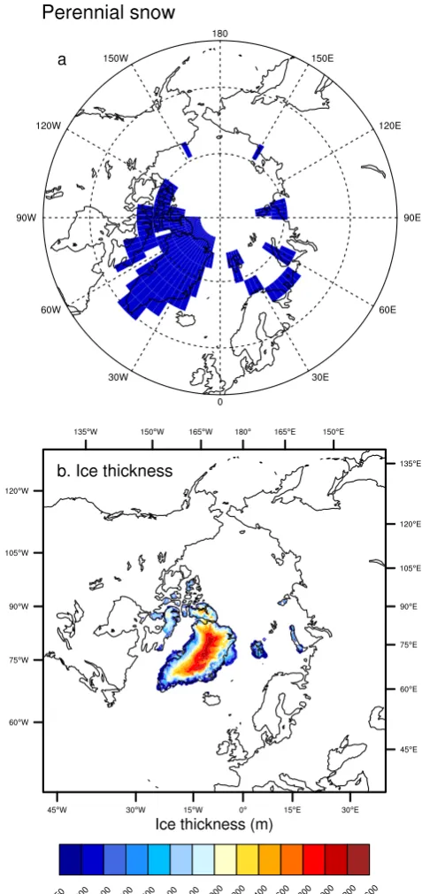
Due to the variations in temperature and precipitation de-scribed above, a perennial snow cover develops in all the experiments but its extent varies according to summer tem-perature and/or precipitation spatial patterns. In K236 and K115, perennial snow is located all along the continental arctic margins, on Svalbard, on the islands of the Barents Sea and Kara Sea and on the Canadian archipelago (Fig. 5b and c). The American Cordilleras are also covered in K115. In contrast, in K125 and K229, the extent of perennial snow is much reduced and is confined exclusively to the eastern part of the Canadian archipelago, Svalbard and the islands of the Barents Sea and Kara Sea (Fig. 5a and d). However, while the extent of perennial snow in K125 is reduced due to the warm summer temperatures, the limited spatial cover in K229 mainly results from a lack of precipitation over the
areas that are covered by perennial snow in K236 (Fig. 4g and h).
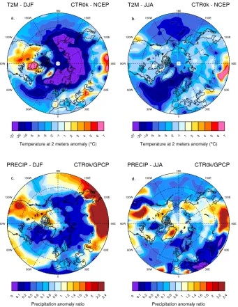
The climatic features described above seem to be realis-tic given the initial conditions (Table 1). However, the low-resolution CESM is affected by some specific biases. The present-day control run CTR0k underestimates temperatures over Northern Eurasia up to 27◦C in winter and by about 3◦C in summer (Fig. 6a and b). This is mainly explained by a weak North Atlantic heat transport towards high latitudes caused by the low spatial resolution (Jochum et al., 2011; Shields et al., 2012). The cold bias over Siberia induces a substantial reduction in precipitation over these regions of at least 90 % during winter and of about 70 % during summer (Fig. 6c and d) if compared to the Global Precipitation Cli-matology Project precipitation data sets (GPCP, Adler et al., 2003). On the contrary, both temperature and precipitation are overestimated over the western part of North America.
Fig. 5. Simulated perennial continental snow cover for each climate experiment, (a) K125, (b) K115, (c) K236 and (d) K229. Snow cover is considered as perennial when residence time is 365 days.
GHGs and SIC albedo feedback (orange curve in Fig. 3b and c). Assuming that the uncertainty on this temperature index is similar to that of our simulated temperatures, this indicates that our two simulations K125 and K115 are able to capture a realistic impact of orbital, GHGs and SIC albedo on temperatures in the Northern Hemisphere. It also suggests that the negative precipitation bias associated with the neg-ative temperature anomaly has a minor impact at that time. However, this might not be the case in K236 and K229 where mean annual temperature anomalies smaller than that of the temperature index. The temperature anomaly is certainly lim-ited by the lack of precipitation inducing a reduction in the snow cover extent in both experiments, which in turn may affect the snow albedo feedback.
3.2 Ice-sheet experiments
In this section we use the simulated air temperature and pre-cipitation previously described to force the GRISLI ISM. In the following the ice volume variations will be expressed in meters sea-level equivalent (m SLE) calculated as
SLE= ρI
ρW
×
N
P
i=1
thki ×1x ×1y 4π R2×A
0
, (7)
whereρI is the ice density (917 g cm−3),ρW is the
seawa-ter density (1018 g cm−3),N is the total number of grid pix-els, thk is the simulated total ice thickness,1x and1y cor-respond to the horizontal grid increment (40 km),R stands for the radius of the earth (3671 km) andA0corresponds to
the present-day surface ratio between oceans and continents (≈0.72).
3.2.1 Steady-state ice-sheets experiments
Fig. 6. Bias in temperature and precipitation in the Northern Hemisphere in the low resolution present-day anthropogenic run CTR0k (Table 1) compared to NCEP reanalysis air temperature (Kalnay et al., 1996) and GPCP precipitation data set (Adler et al., 2003). (a) and (b) simulated winter (DJF) and summer (JJA) air temperature anomaly (◦C) between CTR0k and NCEP reanalysis. (c) and (d) precipitation anomaly ratio (dimensionless) between CTR0k and GPCP precipitation data set.
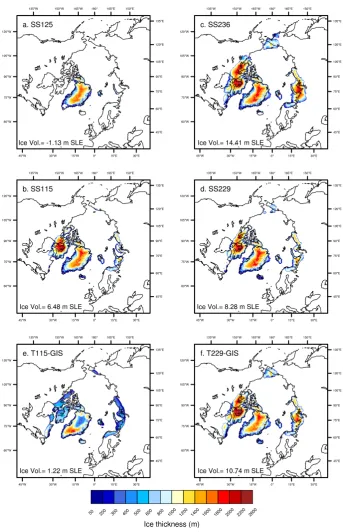
grow correspond to a residence snow time of 365 days per year. In SS236, SS229 and SS115, the main common in-ception areas are covered by ice sheets except in the Cas-cades mountains (Fig. 8b–d). Over this particular region, the CESM underestimates precipitation (Fig. 6), thus limiting the growth of ice in GRISLI. Some mismatch between the peren-nial snow and the ice-sheet distribution in SS236 and SS115 is visible over eastern Siberia as well. This is because the amount of precipitation in K115 and K236 over this region is too low to permit ice-sheet growth in GRISLI. The evolution of ice distribution from SS236 to SS229 and from SS125 to
SS115 is also in agreement with the evolution of simulated perennial snow from K125 to K115 and from K236 to K229. From SS125 to SS115, the ice sheets expand over North America and Eurasia because of temperature drop in K115 relatively to K125. On the contrary, from SS236 to SS229 both North American and Eurasian ice sheets retreat north-ward. This is because precipitation strongly decreases from K236 to K229 over the areas where ice sheets grow, which induces a smaller mass balance in SS229 than in SS236.
SS236 (Fig. 9). In SS125, the simulated final ice volume (i.e., removing about 7.1 m SLE for the present-day Greenland ice sheet) amounts to 1.13 m SLE above present-day mean sea level. In fact, the southernmost part of Greenland melted dur-ing the simulation (Fig. 8a). This result is induced by the orbital configuration at 125 kyr BP (Fig. 2) causing warmer summers than today in K125 by about 1 to 2◦C over Green-land (Fig. 4b). The final ice volume SLE value is in line with the various relative sea-level reconstructions displayed in Fig. 9a (red dot) and is also in agreement with the recent work by Stone et al. (2013) who estimate the contribution of the Greenland ice sheet during the last interglacial to be in the range 0.6 m–3.5 m SLE. The simulated final ice volume in SS236 is about−14.41 m SLE, which also fits the range of the various sea-level reconstructions [−35;−10] m SLE (Fig. 9b).
On the contrary, neither SS229 nor SS115 simulated fi-nal ice volumes match the range of observations. In SS229, the ice volume reaches−8.28 m SLE while observations in-dicate a global sea level of at least−50 m at that time. Sim-ilarly, in SS115, the simulated ice volume is−6.48 m SLE and the sea-level reconstructions indicate a sea level of at least −15 m SLE during that period. The discrepancies be-tween our results and the sea-level reconstructions are, on one hand, due to the fact that in our climate simulations the only feedbacks acting at paleo-timescale are orbitals, green-house gases and the albedo of the sea-ice cover and, on the other hand, due to the uncertainties of the sea-level recon-structions themselves. Moreover, as explained in the previous section, the CESM shows a significant negative temperature bias in the high latitudes, which causes a substantial reduc-tion in precipitareduc-tion.
Since it is difficult to assess the direct impact of such bias in our paleo-ice-sheet simulations, we tested its importance on pre-industrial perennial snow and ice-sheet distribution. Simulated perennial snow cover in CTR1850 is limited to the Canadian archipelago, Svalbard and the islands of Bar-ents Sea and Kara Sea (Fig. 7a). The high latitudes cold bias observed in CTR0k seems to not affect significantly pre-industrial perennial snow cover. What matters most is how the snow cover lasts during the summer. In the case of CTR1850, summer high latitudes insolation is larger by about 40 W m−2 relatively to K115 (Fig. 2a). In addition GHGs are larger in CTR1850 than in K115 (Table 1). Those differences causes a mean summer temperature warming of 3◦C in CTR1850 relatively to K115 over the northern high
latitudes (Fig. 4a). This is enough to melt most of the winter snow over Eurasia and North America and prevent the accu-mulation of an extensive perennial snow cover.
To further investigate the impact in GRISLI, a 150 000 model-years steady-state experiment was per-formed using CTR1850 climatology and using the same parameters as for the paleo-experiments (Sect. 2.2.2). The ice-sheet distribution is in perfect agreement with the simulated perennial snow in CTR1850 (Fig. 7b). The final
Fig. 7. (a) Simulated perennial snow cover as in Fig. 5 from CTR1850 (Table 1). (b) Ice thickness (m) obtained after a 150 000 model year steady-state ice-sheet simulation using a mean annual lapse rate value of 5◦C km−1and a summer lapse rate value of 4◦C km−1.
Fig. 8. Simulated ice thickness (m) for each of the steady-state experiments SS125 (a), SS115 (b), SS236 (c) and SS229 (d). Simulated final ice thickness in meters for the transient experiments T115-GIS (e) and T229-GIS (f). See Table 2 for details. Simulated total ice volume values for each experiment are expressed in meters sea-level equivalent (SLE) and are reported in each frame.
ice-sheet distribution over North America and Eurasia in GRISLI.
Since our climate simulations only account for orbitals, GHGs, and sea-ice albedo, how is it possible that SS125 and SS236 match the relative sea-level observations resulting
−70 −60 −50 −40 −30 −20 −10 0
225 230 235 240
Time (kyrs BP)
f. GIS − +40% precip. −70 −60 −50 −40 −30 −20 −10 0
225 230 235 240
e. GIS
−20 −15 −10 −5 0 5 10
RSL (m.a.s.l.)
110 115 120 125 130
Time (kyrs BP) d. GIS − +40% precip −20
−15 −10 −5 0 5 10
RSL (m.a.s.l.)
110 115 120 125 130
c. GIS
8°C/km 5°C/km no elev. −20
−15 −10 −5 0 5 10
Relative Sea Level (m.a.s.l.)
110 115 120 125 130
Time (kyrs BP) a.
−40 −35 −30 −25 −20 −15 −10 −5 0 5 10
Relative Sea Level (m.a.s.l.)
225 230 235 240
Time (kyrs BP) b.
Fig. 9. Ice volume of steady-state experiments (blue and orange dots) and of transient experiments (thick red line) expressed in relative sea-level (m a.s.l.) for MIS 5 glacial inception period (a) and MIS 7 inception period (b). Red thick line corresponds to transient experiments T115-GIS and T229-GIS ice volume evolution, forced usingIGISindex. Simulated values are compared to various paleo-sea-level observa-tions: Waelbroeck et al. (2002) (black); Siddall et al. (2003) (blue); Shackleton (2000) (brown); Bintanja et al. (2005) (red) and Lea et al. (2002) (orange). Note that sea-level calculation does not account for ice volume developing over the Bering Strait and over the Himalaya areas as observed in our transient experiments (Fig. 8). Time evolution of ice volume of steady-state (empty circles) and transient (continuous and dotted line) experiments expressed in relative sea-level (m a.s.l.) for MIS 5 glacial inception period (c and d) and MIS 7 inception period (e and f). Each steady-state and transient experiment T115-GIS and T229-GIS was repeated three times according to different lapse rate values:λ0= 0◦C km−1(orange) is the case not accounting for elevation changes,λ5◦C= 5◦C km−1for annual temperature and 4◦C km−1
for summer temperatures (red) andλ8◦C= 8◦C km−1and 6.5◦C km−1(magenta). In frames (d) and (f), precipitation was increased by
40 %. Simulated values are compared to various sea-level reconstructions (black empty squares) from Waelbroeck et al. (2002), Shackleton (2000), Bintanja et al. (2005) and Lea et al. (2002). No distinctions have been made between the reconstructions and error bars have been added when available.
that the land-ice albedo feedbacks are not significant com-pared to the other regional feedbacks and suggests that when we simulate climate at times where sea level is equal or higher than present day, the contributions of orbitals and
GHGs to atmospheric temperature are enough to get a rea-sonable continental ice volume that fits with observations.
and the spatial extent of the perennial snow cover would be limited to the region where summer temperature is particu-larly cold (Figs. 4d and 5c). On the contrary, the perennial snow cover is as extensive as in K115 (Fig. 5d) and results from the particularly low level of GHGs which helps main-taining a negative air temperature in K236 (Table 1). Com-pared to K115, precipitation is larger over the inception areas than in K236, which is favorable to a more extended ice-sheet growth in SS236 than in SS115. This is why SS236 final ice volume reaches the upper bound of sea-level obser-vations (Fig. 9b).
3.2.2 Transient ice-sheets experiments
The recent work of Köhler et al. (2010) aimed at calculating the individual contribution of the most important feedbacks acting on paleo-timescale to the mean annual global temper-ature signal: orbitals, GHGs, land-ice, sea-ice, vegetation and aeolian dust. They show that, during interglacials, the land-ice elevation and albedo feedbacks had a minor impact on the mean annual global temperature signal. On the contrary, they point out their increasing importance while climate cools un-til they become the most important contributions to the mean annual temperature signal approaching the glacial maxima. Similarly, with the steady-state experiments, we have shown that depending on the time period simulated, the lack of some of the regional feedbacks induces large discrepancies between simulated and observed/reconstructed past sea-level variations.
To further investigate this issue at those time periods, we performed two transient experiments. The temperature evo-lution between [K236; K229] and [K125; K115] is modu-lated by the index constructed after the works of Köhler et al. (2010) and Quiquet et al. (2013) (see Sect. 2.2.1). TheIGIS
index (Eq. 3) is based on1TGIS which corresponds to the
combined impact of orbitals, GHGs and sea-ice-albedo backs on air temperature (Eq. 2, Fig. 3d and e). These feed-backs are also included in our climate experiments K236, K229, K125 and K115 . . . Details are reported in Sect. 2 and in Table 2.
Ice-sheet distribution
The spatial distribution of the simulated final ice sheets for each of the transient experiments is shown in Fig. 8e and f. In T115-GIS, the final ice-sheet distribution is coherent with that obtained with the steady-state experiment SS115 (Fig. 8e). Ice sheets develop over the Canadian archipelago and south of the Baffin bay as well as over the Norwegian mountain range and the Eurasian Arctic islands (Fig. 8e). The ice over those areas is in general thinner than in SS115, because theIGISindex substantially warms temperatures
be-tween 125 and 121 kyr BP (Fig. 10a and b) preventing ice sheets from accumulating over the inception areas and the accumulation over North America and Eurasia starts only
towards 120 kyr BP. The total accumulation time is then of about 5000 model years against 150 000 model years in the steady-state experiments. Consequently, the ice does not have time to thicken in T115-GIS as much as in SS115.
Similarly to T115-GIS, T229-GIS exhibits an ice-sheet distribution coherent with that obtained with the steady-state experiment SS229 (Fig. 8d and f). At odds with SS115 and T115-GIS, ice domes are thicker over Eurasia and North America in T229-GIS than in SS229. This happens because accumulation in SS229 is lower than in T229-GIS which benefits from the accumulation history since 236 kyr BP (Fig. 10f). Compared to T115-GIS, in T229-GIS ice-sheet dimensions do not vary much from their spin-up geome-try because the climate contrast between K236 and K229 is smaller than between K125 and K115 (Fig. 4). Moreover, the use ofIGIS, whose values fluctuates around 1 (Fig. 3e), does
not induce large additional climatic anomaly in T229-GIS (Fig. 10d and e).
The comparison between T115 and T229 experiments shows that the glacial inception at 229 kyr BP is more de-veloped than at 115 kyr BP, since both North American and Eurasian ice sheets are thicker at 229 kyr BP, while it ap-pears less obvious from the comparison between SS229 and SS115. The only unrealistic feature is the ice accumulation that occurs over the Bering Strait [. . . ] in all the transient experiments (Fig. 8e and f). It has been shown that the exis-tence of an ice sheet large enough over Eurasia could signifi-cantly affect the regional circulation by reducing the mois-ture advection that usually reaches eastern Siberian topo-graphic highs, therefore stopping an ice cap from developing in this area (Krinner et al., 2011). However, the CESM sim-ulations do not account for changes in topography caused by ice-sheet growth and the circulation patterns remain similar in eastern Siberia for all the simulations regardless of the pe-riod. Therefore, since there is no temperature or precipitation effect induced by a deviation in atmospheric circulation in our climate forcing, some ice develops over eastern Siberia in the transient ice experiments.
Comparison with sea-level reconstructions
The time evolution of the ice volume for each transient ex-periment is displayed in Fig. 9a and b. As expected, the ice volume evolution follows the main trends of the tem-perature index. In T115-GIS the ice volume first decreases until 121 kyr BP and then increases with cooling temper-ature (Fig. 9a). For T229-GIS, ice volume is stable until 231 kyr BP and slightly decreases until the end of the simu-lation becauseIGISinduces a slight warming in temperature
from this time (Fig. 10b and e).
−28 −24 −20 −16 −12 −8
Tann (°C)
116 118 120 122 124
Eurasia
8°C/km 5°C/km no elev.
North Am.
a.
−8 −4 0 4 8 12
Tjja (°C)
116 118 120 122 124
b.
0.2 0.3 0.4
Accum. (m/yr)
116 118 120 122 124
Time kyrs BP c.
−40 −36 −32 −28 −24 −20 −16
230 232 234 236
d.
−24 −20 −16 −12 −8 −4 0 4
230 232 234 236
e.
0.2 0.3 0.4
230 232 234 236
Time kyrs BP
f.
Fig. 10. Mean annual temperatures, July temperatures and mean annual precipitations time series resulting from Eqs. (5) and (6). Time series account for different lapse rates values:λ0= 0◦C km−1is the case not accounting for elevation changes,λ5◦C= 5◦C km−1for annual
temperature and 4◦C km−1for summer temperatures andλ8◦C= 8 and 6.5◦C km−1. Time series are displayed for MIS 5 (a, b and c) and
for MIS 7 (d, e and f) time periods and show the climate evolution for Eurasia (red/orange colors) and North America (blue/cyan colors). Note that precipitation does not depend on the lapse rate, this is why there is only one time serie displayed for Eurasia (red), averaged over the Barents and Kara Seas, and North America (blue), averaged over the Hudson Bay and the Canadian archipelago.
enough to cause an increase in accumulation which com-pensates for the 150 000 model-year accumulation time of SS115 (blue dot). T229-GIS highly underestimates obser-vations by more than 20 m SLE (Fig. 9b). The steady-state experiment SS236, together with sea-level reconstructions, suggests that some ice sheets probably already existed at this time period. In our climate simulation K236 we did not pre-scribe ice sheets over the inception areas. For that reason, simulated temperatures in K236 might be overestimated (i.e., too warm) compared to a climate simulation accounting for SS236 ice-sheet distribution as an initial condition. In addi-tion, sea-level reconstructions suggest that ice sheets further developed until 229 kyr BP. The lack of prescribed ice sheets in climate simulation K229 also contributes to overestimate temperatures at this time, which is also supported by Quiquet et al. (2013) temperature index (Fig. 3c). The mismatch with paleo-observations is probably caused by a low accumulation resulting from the negative precipitation bias occurring over the inception areas in K229 climate forcing. This bias is fur-ther amplified by the precipitation scheme used in GRISLI (Eq. 6). The precipitation scheme follows the formulation of Greve (2005) which approximates the saturation vapor pres-sure in the atmosphere. In other words, this means that pre-cipitation in GRISLI decreases with deceasing temperature,
and if temperatures are particularly cold, precipitation will be particularly low. The impact of precipitation bias, strength-ened by the precipitation scheme of GRISLI, might strongly limit the ice accumulation in MIS 7 experiments.
3.2.3 Lapse rate and precipitation impact on ice-sheet distribution
The steady-state and transient experiments described in the previous sections account for a mean annual lapse rate of 5◦C km−1and a summer lapse rate of 4◦C km−1(hereafter,
λ5◦C). To test the sensitivity of our simulations to lapse rate
values, we performed two series of new steady-state and transient experiments similar to those described in Table 2 but (1) using a winter and summer lapse rates of 8 and 6.5◦C km−1(hereafter,λ
8◦C) and (2) not accounting for
ele-vation changes (both lapse rates set to 0,λ0). Finally, all the
transient experiments accounting for the three sets of lapse rate,λ8◦C,λ5◦C,λ0, were run again increasing precipitation
0 1 2 3 4 5 6 7
Ice sheet area (10
6 km 2)
116 118 120 122 124
e. +40% precipitation
0 1 2 3 4 5 6 7
Ice sheet area (10
6 km 2)
230 232 234 236
f. +40% precipitation −8
−6 −4 −2 0 2 4
I(t)
116 118 120 122 124
c.
−2 0 2 4
I(t)
230 232 234 236
d. 0
1 2 3 4 5 6 7
Ice sheet area (10
6 km 2)
116 118 120 122 124
Time (kyrs BP)
Eurasia GIS 8°C/km 5°C/km no elev.
North Am. GIS 8°C/km 5°C/km no elev.
a.
0 1 2 3 4 5 6 7
Ice sheet area (10
6 km 2)
230 232 234 236
Time (kyrs BP)
b.
Fig. 11. Impact of lapse rate and precipitation formulation on ice-covered area of individual North American (blue colors) and Eurasian (red colors). Each transient experiment T115-GIS and T229-GIS was repeated three times according to different lapse rate values:λ0= 0◦C km−1 is the case not accounting for elevation changes,λ5◦C= 5◦C km−1for annual temperature and 4◦C km−1for summer temperatures and λ8◦C= 8 and 6.5◦C km−1. Results corresponding to Fig. 8c–d are plotted using red curves and in top frames. In frames (a) and (b),
precip-itation formulation from Greve (2005) was used while in frames (e) and (f), precipprecip-itation was increased by 40 %. In addition, in frames (c) and (d)IGISfor both MIS 5 and MIS 7 time periods is displayed as in Fig. 3e and f.
of lapse rate and precipitation on the time evolution of ice volume (Fig. 9c–f) and ice area (Fig. 11).
For MIS 5 time period, the use of different lapse rates does not impact on the expansion rate of both ice sheets (Fig. 11a and e). The general shape of the curves is also well correlated to the shape ofIGIS(Fig. 11c). Note that ice starts expanding
over North America and Eurasia only after 121 kyr BP be-cause summer temperature is highly positive until this time causing a larger amount of ice melting (Fig. 10b). In addi-tion, the North American ice sheet final area is larger than the Eurasian one (Fig. 11a) which suggests that in order to expand the Eurasian ice sheet, temperatures colder than those obtained usingIGIS are needed. In fact, mean annual
and summer temperatures over North America are lower than over Eurasia starting at 120–119 kyr BP (Fig. 10a and b).
When considering an overall increase of precipitation, fi-nal area over Eurasia has increased by 75 % and by about 45 % over North America (Fig. 11e). The Eurasian ice sheet is thus more sensitive to the lack of precipitation than the North American one, which might be related to the precip-itation bias detected in CESM which is particularly strong over the Eurasian inception areas (Fig. 6c and d). However, increasing precipitation does not increase ice-sheet sensitiv-ity to the various lapse rates (Fig. 11b).
discrepancies in the ice areas over both North America and Eurasia: the largest ice area corresponds to the largest lapse rate valueλ8◦C(Fig. 11b and f). Both ice sheets are
retreat-ing (Fig. 11b) and the lower theλ, the larger the retreat. This behavior has a two fold explanation. First there is a reduction in precipitation caused byIGIS along with a slight cooling
of temperatures. Second, this cooling does not increase the area of possible ice accumulation contrary to what happens in T115-GIS (Fig. 10d–f). In contrast with T115-GIS experi-ments, increasing precipitation induces larger ice-sheet areas for both North America and Eurasia and enhances the dif-ferences obtained using the different lapse rates (Fig. 11f). Consequently, both ice sheets expand instead of retreating (Fig. 11f).
The impact of lapse rates is more important on MIS 5 ice volume than on MIS 5 ice area (Fig. 9c and d). First, steady-state experiments differ by about 5 m SLE between the largest lapse rateλ8◦C and the case with no elevation
changes accounted forλ0 (Fig. 9c, circles). In addition, the
various sets of transient experiments differ from 125 kyr BP to≈119 kyr BP and the twoλ8◦Candλ5◦Clapse rates
con-tribute to the melting of more than half of the initial ice volume in SS125, while λ0 only produces limited
melt-ing (Fig. 9c and d). After 119 kyr BP, no substantial differ-ence is observed between the various lapse rates. This hap-pens because temperature does not favor accumulation be-fore 121 kyr BP (1Ttopo in Eq. 5 equals 0). Nevertheless, in
the T115-GIS experiments, increasing precipitation leads to a larger final ice volume, reaching the values of the steady-state experiments (Fig. 9d). This suggests that the larger precipita-tion compensates for the long accumulaprecipita-tion time of SS115. However, while T115-GIS almost reaches the upper bound of paleo-observations, increasing precipitation together with prescribing a larger lapse rate value is not enough to gener-ate a cooling which would allow ice volume to better match paleo-observations.
For MIS 7 experiments, the impact of the various lapse rates induces larger differences between the various steady-state simulations than in MIS 5 experiments (Fig. 9e). In fact, transient ice volume differs by 10 m SLE between the cases using λ0 and the largest lapse rate value. This is twice as
large as the difference generated by the different lapse rates in the transient experiments of MIS 5 time period. Contrary to what is obtained in T115-GIS, the lower bound of ice vol-ume is given by the simulation discarding the elevation effect while the upper bound is given byλ8◦C(Fig. 9e and f). This
is due to the fact that temperature anomaly between 236 and 229 kyr BP always remains negative over inception areas and especially during summer while this is not the case between 125 and 115 kyr BP (Fig. 10). As a consequence, ice volume in T229-GIS simulations is always larger than present-day Northern Hemisphere ice volume. Similarly to T115-GIS, T229-GIS ice volumes do not fit with paleo-observations in-dicating that in this case, cooling alone is not enough to foster accumulation.
With larger precipitations, T229-GIS ice volumes still un-derestimate the observations by about 20 m SLE (Fig. 9e and f). The precipitation during MIS 7 is similar to MIS 5 over Eurasia but temperatures are much lower (Fig. 10). However, the final areas are almost the same for both time periods (Fig. 11e and f). which indicates that despite the cold temperatures, an increase of 40 % in precipitation is not enough to generate a larger ice volume and a larger ice area in the MIS 7 experiments that fit with paleo-observations. This suggests that for MIS 7 the lack of precipitation caused by the high-latitude temperature bias in CESM is mainly re-sponsible for this discrepancy in ice volume.
4 Discussion
With two types of ice-sheet experiments, steady state and transient, we wanted to test the impact of external forcing (orbitals and GHGs) on the growth of ice sheets during the last two glacial inceptions. What we have shown in this work is that the steady-state ice distribution at both inception times differs from the transient one. The steady-state exper-iments (i.e., forced by steady-state simulated climates) un-derestimate the ice volume at both inceptions times (229 and 115 kyr BP), while the pre-inception simulated ice volumes (236 and 125 kyr BP) are in good agreement with observa-tions. While increasing precipitations allows MIS 5 experi-ments to almost reach the upper bound of paleo-observations, for MIS 7, on the contrary, ice volume is underestimated, independently from the lapse rate value and the amount of precipitation. This suggests that the lack of precipitation de-tected in our CESM climate simulations, combined with the already cold MIS 7 climate induced by the external forcing over the inception areas stops the ice sheets from expanding and thickening at that time. Our conclusion is that cold biases are more effective during a cold inception, such as during MIS 7, than during a warm inception, such as MIS 5.
albedo feedback, CO2, insolation feedback and a residual
term (Köhler et al., 2010, followed a similar approach). In their dynamical ice-sheet model, accumulation is based on present-day observations which are modulated, through a power law, by the simulated surface temperature anomaly be-tween two time periods. As in Charbit et al. (2002), the fact that this method is based on present-day climatology allows removal of climate model potential biases. As a result, Abe-Ouchi et al. (2007) were able to broadly reproduce a sea-level drop of about 130 m for the LGM (21 ky BP), using a lapse rate of 5◦C km−1, in agreement with observations.
On the contrary, in our case, we deliberately use the sim-ulated temperature and precipitation as reference climate to evaluate the capability of CESM with GRISLI to properly simulate different glacial inceptions. Furthermore, the fact that we use both steady-state and transient experiments al-lows us to highlight several important issues for both climate modeling and ice modeling. First of all, the steady-state ice experiments are very useful to understand the limits of cli-mate forcing input in terms of temperature and precipitation. In all numerical models, a spin-up of the simulated variables is necessary, especially when thermodynamics is an active part of the simulated processes. However, in nature, the state of the earth’s system at a given time depends on its evolution. This is particularly important for the components of the sys-tem that have long-term memory of climate changes, such as the deep ocean, the ice sheets and ice caps. Our results show that ISM steady-state experiments are efficient when the feedbacks accounted for into the climate simulations are likely to be the dominant feedbacks active during the epoch considered. In the case of our “interglacial” simulations at 125 and 236 kyr BP, orbitals, GHGs and the sea-ice albedo feedbacks are enough to simulate a reasonable steady-state ice distribution. On the other hand, both steady-state and transient experiments show that for the inception simulations at 115 and 229 kyr BP, those three feedbacks are not enough to give an ice volume which fits with the observations. The combination of steady-state and transient ice experiments is highly powerful in our case to evidence the limits and biases of our models combination.
As we showed, our present-day anthropogenic climate simulation (CTR0k) presents strong winter negative temper-ature bias over the Eurasian inception areas causing a re-duction in precipitation. If we assume that the cold bias was likely propagated into our past climate simulations, it could have affected the inception process in GRISLI (i) by enhanc-ing the glacial inception, as previously shown in Vettoretti and Peltier (2003), and/or (ii) by resulting in a significant reduction in precipitation over the Eurasian Arctic regions. However, our transient simulations show that those biases do not have the same importance during MIS 5 and MIS 7 and that their contribution depends on the mean background cli-mate state of the epoch considered. Indeed, in our “warm” glacial inception (MIS 5), the high summer temperature at 125 kyr BP inhibits the growth of ice sheets despite the
negative temperature bias in the high latitudes, because at that time it is the impact of precession on high latitude cli-mate that mostly matters. On the other hand, in our “cold” glacial inception (MIS 7) the summer temperature is partic-ularly low, due to the low level of GHGs, and causes the cli-mate to be particularly dry. In this case, the dryness strength-ens the negative precipitation bias by limiting the amount of ice accumulating over the high latitudes.
To improve those results, an alternative approach could be to apply a correction on precipitation and/or tempera-tures over the regions affected by the biases. Some previ-ous studies using coupled ice-sheet–climate models tested the implementation of “patches” for precipitation over the ar-eas of inceptions to counteract the climate model bias (e.g., Bonelli et al., 2009; Ganopolski et al., 2010). However, ap-plying patches over some particular areas greatly limits the validation of the capability of coupled systems to reproduce glacial inceptions where the geological evidence indicate the presence of past ice sheets. It unnaturally forces the response of the climate and ice-sheet models. Moreover, it also lim-its investigations of whether coupled systems are able to re-produce different spatial ice-sheet distributions during older glacial cycles. This solution might be applied only if the aim of the numerical experiments is beyond the scope of validat-ing and calibratvalidat-ing the models to improve the simulation of climate processes.
A last caveat concerns the resolution of the CESM sim-ulations. Compared to Jochum et al. (2011), we simulated the same glacial inception (≈115 kyr BP) starting from a colder mean ocean state spin-up (here 125 kyr BP) and with a coarser horizontal resolution (T31). As a result, the simu-lated perennial snow cover seems to be slightly less extensive at lower resolution, implying that resolution is important for the simulation of polar processes as suggested in the previ-ous work of Vavrus et al. (2011). Simulating the climate at a higher spatial resolution would likely improve the glacial in-ception in the climate models, especially over high topogra-phies where numerous GCMs usually fail to calculate cor-rect precipitation patterns (Bonelli et al., 2009). It would also contribute to resolve the melting processes along the margins of the ice sheets, which are critical for the advance and/or re-treat of the ice sheets over continental areas laying below a certain latitude (e.g., Colleoni et al., 2009b).