in Multivariate Stratified Sampling
Ummatul Fatima
Department of Statistics and Operations Research Aligarh Muslim University, Aligarh 202002, India [email protected]
M. J. Ahsan
Department of Statistics and Operations Research Aligarh Muslim University, Aligarh 202002, India
Abstract
Consider a multivariate stratified population with L strata and p1 characteristics. Let the estimation of the population means be of interest. In such cases the traditional individual optimum allocations may differ widely from characteristic to characteristic and there will be no obvious compromise between them unless they are highly correlated. As a result there does not exist a single set of allocations (n1,n2,...,nL) that can be practically implemented on all characteristics. Assuming the characteristics independent many authors worked out allocations based on different compromise criterion such allocations are called compromise allocation. These allocations are optimum for all characteristics in some sense. Ahsan et al. (2005) introduced the concept of ‘Mixed allocation’ in univariate stratified sampling. Later on Varshney et al. (2011) extended it for multivariate case and called it a ‘Compromise Mixed Allocation’. Ahsan et al. (2013) worked on mixed allocation in stratified sampling by using the ‘Chance Constrained Programming Technique’, that allows the cost constraint to be violated by a specified small probability. This paper presents a more realistic approach to the compromise mixed allocation by formulating the problem as a Chance Constrained Nonlinear Programming Problem in which the per unit measurement costs in various strata are random variables. The application of this approach is exhibited through a numerical example assuming normal distributions of the random parameters.
Keywords: Multivariate stratified surveys, Compromise mixed allocation, Chance constrained programming.
Mathematics Subject Classifications 62D05 62H12
1. Introduction
In stratified sampling, the use of any particular type of allocation depends on the nature of the population, objectives of survey, the available budget, etc. Practically, there are situations where all strata of a stratified population do not allow the use of a single type of allocation. For example, in the absence of the strata weight Wh, strata variance Sh2 and per unit measurement cost ch;h1,2,...,L, optimum allocation can not be used. Similarly, if strata sizes Nh;h1,2,...,L are unknown proportional allocation can not be used. Thus, when no information about some strata of the population is available, ‘equal’ allocation may be used for a given total sample size for that strata. If the only information available for some strata is Nh, ‘proportional’ allocation may be used, that is, nhNh. If
2 h
sample unit does not vary considerably over some strata, an allocation nhWhYh may be used. As the range Rh of a stratum provides an approximation to the standard deviation in the absence of the knowledge of the stratum standard deviations Sh, the allocation may be taken as nhWhRh (See Murthy (1967)). When full information about the population is available, the obvious choice is the ‘optimum allocation’. Ahsan et al. (2005) divided the strata into disjoint groups and used different allocations for different groups. They called their allocation as ‘Mixed Allocation’. Later on Varshney and Ahsan (2011) extended the work of Ahsan et al. (2005) for multivariate stratified sampling. Ahsan et al. (2013) worked out mixed allocation using chance constraint that allows the cost constraint to be violated by a specified small probability.
In this paper the work of Ahsan and Naz (2013) is extended for multivariate stratified sampling, where in cost constraint, a small probability of violation is allowed. Because per unit cost of measurement ch;h1,2,...,L may vary during the course of the survey due to random causes in practice it becomes a random variable. Thus the problem of compromise mixed allocation can be viewed as a Chance Constrained Nonlinear Programming Problem (CCNLPP).
In section 2 and 3 the work of Varshney et al. (2011) and Ahsan et al. (2013) are summarized for the sake of continuity.
2. Compromise mixed allocation
Let the Lstrata of a multivariate stratified population be divided into k groups
k G G
G1, 2,..., , where the group Gj;j1,2,...,k consists of Lj strata with
k j
j L L 1
. The
strata are grouped according to the information available for them, that is, full information partial information or zero information (See Kozak (2006(a), 2006(b))). Or according to some other measure of information as desired in the ‘Introduction’ of this manuscript.
Without loss of generality we can assume that the first L1strata constitute the group G1, the next L2strata constitute the group G2, and so on. The last Lk strata will constitute the groupGk. In order to use different types of allocations in different groups define
k j
I h
nhjh; j; 1,2,..., (2.1)
where Ij;j 1,2,...,k is the set of indices of the strata constituting the group Gj, k
j I h j
h; ; 1,2,...,
are known constants depending upon the type of allocation to be
used in the group Gj and j;j 1,2,...,k are the decision variables to be determined. For example if in any particular group, say Gp, equal allocation is to be used then
I h
1;
q h h W ;hI
, for optimum allocation in the rth group Gr, hmay be taken as r
h h h
h W S / c ;hI
and so on.
It is to be noted that under the above scheme
k j L L L I j i i j i i j i i
j 1, 2,..., ; 1,2,..., 1 1 1 1 1
(2.2) where
I r sIr s ; and {1,2,..., } 1 L I k j j
Using compromise criterion of Yates (1960), Varshney and Ahsan (2011) formulated the problem of finding a compromise mixed allocation as the following Nonlinear Programming Problem (NLPP) for multivariate stratified sampling as
k
j h I j h lh h p l l j S W a 1 2 2 1 M inimize (2.3) 0 1 to
subject c C
k j h I
h h j j
(2.4)and N h Ij j k
h h j h ,..., 2 , 1 ; ; 2 (2.5)
where al 0;l 1,2,...,p are weights associated to the lth characteristics according to its relative importance, ch is the cost of measuring all the p characteristics on a selected unit of the hth stratum, that is, lh
p l
lh
h c h L c
c ; 1,2,..., ,
1
denote the per unit cost of
measuring the lth characteristic in the hth stratum. Without loss of generality we can assume that
p l l a 1 1.
Using Lagrange multipliers technique Varshney and Ahsan (2011) obtained the values of
j
as
k j c A c A C k
j h I
h h I h h h I h h h I h h h j j j j j ,..., 2 , 1 ; 1 0
(2.6)where ; 1,2,..., .
1 2 2
p l lh l hh W a S h L
3. Chance constrained mixed allocation
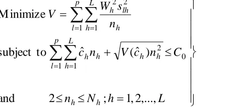
Ahsan and Naz (2013) formulated the mixed allocation that minimizes the variance of the stratified sample mean for a fixed cost as the following CCNLPP
k
j h I j h lh h j
j S W F
1
2 2 )
( M inimize
(3.1)
0 0 1
to
subject P c C p
k j h I
h h j j
(3.2)
and j 0;j 1,2,...,k
(3.3)
Where ~ ( , 2 )
h
h c
c h N
c because in a survey if the costs for enumerating a characteristic in various strata are not known exactly and these are being estimated from sample costs that may be subjected to random variations. They may increase to a level where the cost constraint is violated.
The chance constraint (3.2) may be expressed as
0 0 1
p C q
P k j h I
j h j
(3.4)
where ~ ( , 2 2 )
h
h h c
c h h
h
h c N
q
Define d0as
k
j h I j h j
q d
1
0 (3.5)
Since qh are normally distributed and j are unknown constants, d0 will also be normally distributed with a mean
k
j h I j h j
q d
1
0 (3.6)
and variance
k
j h I
h j k
j h I j h
j j
q V q
V d V
1 2
1
0) ( )
(
(3.7)
Using (3.5), (3.6) and (3.7) the constraint (3.4) can now be expressed as
0 0 0 ]
[d C p
P
0
0 0 0
0 0 0
) ( )
( V d p
d C d V
d d
P
0
0 0 0
)
(d p
V d C Z
P
(3.8)
where Z ~ N(0,1).
Thus the probability of realizing d0 smaller than or equal to C0 can be written as
) ( 0
0 0 0
0
d V
d C C
d
P (3.9)
where (x) represents the cumulative distribution function of the standard normal variate evaluated at x.
If 0 denotes the value of the standard normal variable at which (0) p0 then the constraint (3.8) implies that
) ( )
( 0 0
0
0
d V
d C
(3.10)
Inequality (3.10) will be satisfied if and only if
0 0
0 0
) (
d V
d C
d00 V(d0)C0 0
(See Rao S. S. (2010)).
Using (3.6) and (3.7), we get
0 )
( 0 0
0 1
C d V q
k j h I
j h j
or ( ) 0 0
1 2 0
1
C q V q
k j h I
h j k
j h I j h
j j
(3.11)
Inequality (3.11) gives the deterministic equivalent to the linear chance constraint (3.4).
Thus the solution of the stochastic nonlinear programming problem (3.1)-(3.3) can be obtained by solving the equivalent deterministic programming problem
k
j h I j h h h j
j S W F
1
2 2 )
( M inimize
0 )
( to
subject 0
1 2 0
1
C q V q
k j h I
h j k
j h I j h
j j
(3.13)
and j 0;j 1,2,...,k
(3.14)
Problem (3.12)-(3.14) is a nonlinear programming problem and could be solved by a suitable nonlinear programming technique. Ahsan and Naz (2013) used the optimization software LINGO (2001) to obtain a solution.
4. Chance constrained compromise mixed allocation
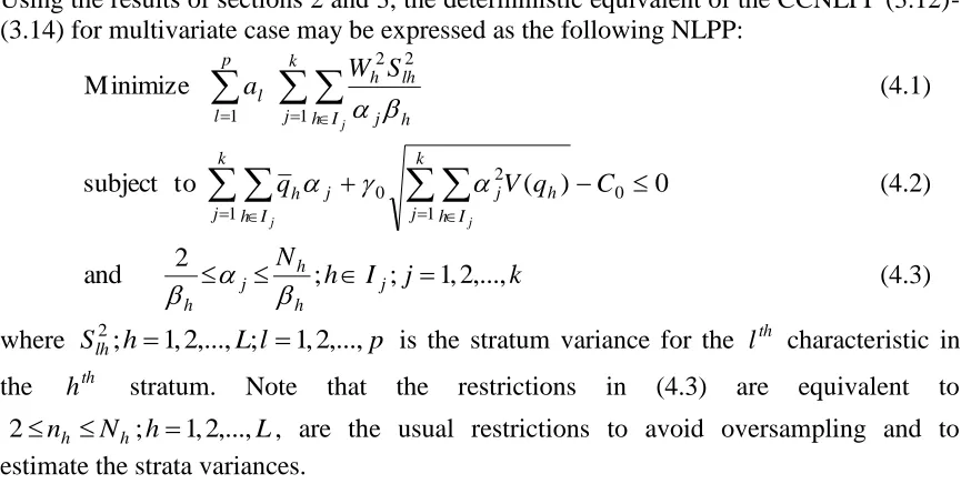
Using the results of sections 2 and 3, the deterministic equivalent of the CCNLPP (3.12)-(3.14) for multivariate case may be expressed as the following NLPP:
k
j h I j h lh h p
l l
j S W a
1
2 2
1 M inimize
(4.1)
0 )
( to
subject 0
1 2 0
1
C q V q
k j h I
h j k
j h I j h
j j
(4.2)
and N h Ij j k
h h j h
,..., 2 , 1 ; ;
2
(4.3)
where Slh2;h1,2,...,L;l 1,2,...,p is the stratum variance for the lth characteristic in the hth stratum. Note that the restrictions in (4.3) are equivalent to
L h
N
nh h; 1,2,...,
2 , are the usual restrictions to avoid oversampling and to estimate the strata variances.
When the numerical data are available the NLPP (4.1)-(4.3) may be solved using a suitable Nonlinear Programming Technique. In the next section an application of the proposed formulation is given for an artificial data. The solution to the NLPP (4.1)-(4.3) is obtained by the optimization software LINGO (2001).
5. A numerical illustration
Varshney et al. (2011) gave a numerical illustration using an artificial data given in Table 1.
The values of ˆ2
h
c
areassumed by authors. The available amount C0 for measurements is
2000 units. This amount is bifurcated in proportion to
4
1 1 h
h
c and
4
1 2 h
h
c approximately
as C011160 and C02840 for the first and second characteristics respectively.
The grouping scheme and values of h,hIj;j1,2,...,k are same as given in Varshney et al. (2011).
Table 2 Expected cost with their estimated variances for the two characteristics
The authors assumed that the probability of violation of the cost constraint is 0.01, that is, the cost of constraint should be satisfied with probability 0.99. This gives the value of 0 as 2.33 from standard normal area table.
The strata are so numbered that:
(i) Strata 1, 2 and 3 constitute group G1 in which equal allocation is to be used, that is }
3 , 2 , 1 { ;
1 1
h I
h
(5.1)
(ii) Strata 4 and 5 constitute group G2 in which proportional allocation is to be used, that is
} 5 , 4 { ; 2
Wh h I
h
(5.2)
(iii) Strata 6 and 7constitute group G3 in which optimum allocation is to be used, that is
2 , 1 }; 7 , 6 { ;
/ 3
1 2
2
l I
h c S a W
p l
lh lh l h h
(5.3)
(See Varshney et al. (2011)).
It can be seen that Ij;j 1,2,3 are mutually exclusive and exhaustive.
It is also assumed that both the characteristics are equally important, that is, 5
. 0 2 1 a
a .
Using (5.1), (5.2) and (5.3) the values of h;h1,2,...,7 are obtained as 1
3 2
1
, 4 0.0872, 5 0.0932, 6 1.0301 and
7121 . 1 7
(5.4)
Using the values given in the Table 1 and Table 2 and the values of h given in (5.4) the NLPP (4.1)-(4.3) may be expressed as
Minimize ()
3 2
1
79198771 .
16 4232983 .
139 5.26270853
(5.5)
subject to
2112.07162 35.98253
+2.33 58 12 0.55710992 2 216.7032762 32 2000
2
(5.6)
0 1
0 2
(5.7)
0 3
Using optimization software LINGO the solution to the NLPP (5.5)-(5.7) is obtained as:
60410 . 13 1
, 2 211.1268 and 315.97107.
Expression (2.1) give the rounded off compromise mixed allocation for the computed values of j; j1,2,3 as
14 60410 . 13 1 3 2
1n n n
18 41025 . 18 08720 . 0 1268 . 211 4
2
4
n
20 67701 . 19 09320 . 0 1268 . 211 5
2
5
n
16 45179 . 16 0301 . 1 97107 . 15 6 3
6
n
27 34406 . 27 7121 . 1 97107 . 15 7 3
7
n .
The total sample size 123 7
1
h
h n
n (5.4)
Under the above (rounded off) compromise mixed allocation the estimated variances )
(ylst
v (ignoring fpc) for the two characteristics are v(y1st)1.653680948 and 561467036
. 2 ) (y2st
v with a trace value 4.215147984.
6. A Comparative study
The allocations compared are
1. Proportional allocation
2. Cochran’s compromise allocation
3. Chatterjee’s compromise allocation
4. Sukhatme’s compromise allocation
5. Proposed compromise mixed allocation
6.1 Proportional allocation
With total sample size n123 as given in (5.4), the rounded off proportional allocation will be
, 16 ,
11 ,
11 ,
21 ,
28 ,
23 2( ) 3( ) 4( ) 5( ) 6( )
) (
1 prop n prop n prop n prop n prop n prop
n
13 ) ( 7 prop
n
with variances ignoring fpc as Vprop(y1st)2.619337334, Vprop(y2st)3.881857529. The trace value is 6.501194863.
6.2 Cochran’s average allocation
p l L h N n C n c V n c n s W V h lh l lh lh lh L h lh L h lh lh h l ,..., 2 , 1 ; ,..., 2 , 1 ; 2 ) ˆ ( ˆ to subject M inimize 0 2 0 1 1 2 2
(6.1)where C0l denote the amount assigned for measuring the lth characteristics; l 1,2,...,p. Let n*l (nl*1,nl*2,...,nlL* ) denote the solution to the lth NLPP in (6.1) with Vl* as the value of the objective function.
Cochran’s compromise allocation is then given by
p l lh a h n p n 1 * ) ( 1; h1,2,,L (6.2)
where the suffix ‘a’ stands for ‘Average allocation’.
With the available data (6.2) give the rounding off average allocation as
) 24 , 15 , 17 , 16 , 10 , 13 , 12 ( ) (a
n .
With variances (ignoring fpc) as Va*(y1st)1.869742767 and Va*(y2st) 2.913005764. The ‘Trace’ is 1.869742767 2.913005764 4.782748531.
6.3 Chatterjee’s compromise allocation
Chatterjee (1967) obtained the compromise allocation by minimizing the sum of the relative increase El in the variances of the estimates ylst of the population means
p l
Yl; 1,2,..., .
Chatterjee formulated the problem as
,..., 2 , 1 ; 2 and ) ˆ ( ˆ to subject ) ( ˆ 1 M inimize 0 2 1 1 1 2 * 0 1 L h N n C n c V n c n n n c C E E h h h h L h h h p l L h h h lh h p l l (6.3)With available data the Chatterjee’s compromise allocation (rounded off) are obtained as: 24
, 15 ,
17 ,
17 ,
09 ,
13 ,
12 2 3 4 5 6 7
1 n n n n n n
n . With variances (ignoring fpc)
as VC(y1st)1.860335122, VC(y2st) 2.906798467 and a trace value of 4.767133589, where ‘C’ stands for Chatterjee.
6.4 Sukhatme’s compromise allocation
Sukhatme et al. (1984) obtained the compromise allocation by minimizing the sum of the variances for the p characteristics under linear cost constraints. The NLPP for this allocation is given as:
,..., 2 , 1 ; 2
and
) ˆ ( ˆ
to subject M inimize
0 2
1 1 1 1
2 2
L h
N n
C n c V n c
n s W V
h h
h h h
p l
L h
h p l
L
h h
lh h
(6.4)
Using the values given in Table 1 and 2 the rounded off solution to NLPP (6.4) is given as
27 ,
17 ,
19 ,
18 ,
11 ,
15 ,
14 2 3 4 5 6 7
1 n n n n n n
n with the objective value as
4.240085924 which is also the trace value.
7. Summary of the Results
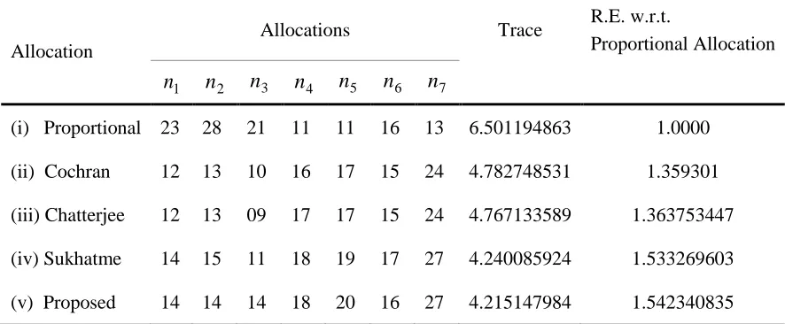
Table 3 gives the summary of the results of the numerical illustration.
Table 3 Summary of the results
The last column of Table 3 provides the Relative Efficiencies (R.E.) of the four compromise allocations as compared to the proportional allocation. It can be seen that the proposed allocation is the most efficient among the considered allocations.
Acknowledgement
The author Mohammad Jameel Ahsan is grateful to the UGC for its financial support in the form of Emeritus Fellowship in the preparation of this manuscript.
References
1. Ahsan, M.J., Najmussehar, Khan, M.G.M. (2005). Mixed allocation in stratified sampling. Aligarh J. Statist. 25, 87-97.
2. Ahsan, M.J., Naz, F. (2013). Chance constrained mixed allocation. International J. Innovative Tech. Res. Volume No. 1, Issue No. 5, 398-401.
4. Cochran, W.G. (1977). Sampling Techniques. John Wiley, New York.
5. Kozak, M. (2006a). On sample allocation in multivariate surveys. Comm. Statist. Simulation Comput. 35, 901-910.
6. Kozak, M. (2006b). Multivariate sample allocation: application of random search method. Statistics in Transition 7(4), 889-900.
7. LINGO: LINGO-User’s Guide. (2001). Published by LINDO SYSTEM INC., 1415, North Dayton Street, Chicago, Illinois, 60622, USA.
8. Murthy, M.N. (1967). Sampling Theory and Methods. Statistical Publishing Society, Calcutta.
9. Rao, S.S. (2010). Engineering Optimization: Theory and Practice. (3rd Edition) New Age International Publishers, New Delhi.
10. Sukhatme, P.V., Sukhatme, B.V., Sukhatme, S., Asok, C. (1984). Sampling Theory of Surveys with Applications. Iowa State University Press, Iowa, U.S.A. and Indian Society of Agricultural Statistics, New Delhi, India.
11. Varshney, R., Ahsan, M.J. (2011). Compromise mixed allocation in multivariate stratified sampling. J. Indian Soc. Agr. Stat. 65(3), 291-296.
Table 1: Data for seven strata and two characteristics
h Nh Wh s1h s2h
1 2 3 4 5 6 7
472 559 425 218 233 328 265
0.1888 0.2236 0.1700 0.0872 0.0932 0.1312 0.1060
05.237 05.821 05.238 25.528 22.232 15.129 40.125
07.815 07.949 07.725 30.125 32.231 18.455 45.358
Table 2: Expected cost with their estimated variances for the two characteristics
h cˆ 1h cˆ 2h cˆh cˆ1h cˆ2h 2
1
ˆ
h
c
2
2
ˆ
h
c
2 2 2
2 1 ˆ
ˆ ˆ
h h
h c c
c
1 2 3 4 5 6 7
3 5 4 7 6 6 9
3 3 3 5 5 4 6
6 8 7 12 11 10 15
6 7 8 11 15 17 20
10 12 15 20 22 27 38
16 19 23 31 37 44 58
Table 3: Summary of the results
Allocation
Allocations Trace R.E. w.r.t.
Proportional Allocation
1
n n2 n3 n4 n5 n6 n7
(i) Proportional 23 28 21 11 11 16 13 6.501194863 1.0000
(ii) Cochran 12 13 10 16 17 15 24 4.782748531 1.359301
(iii) Chatterjee 12 13 09 17 17 15 24 4.767133589 1.363753447
(iv) Sukhatme 14 15 11 18 19 17 27 4.240085924 1.533269603