Climate of the Greenland ice sheet using a high-resolution climate model – Part 1: Evaluation

(1)

www.the-cryosphere.net/4/511/2010/ doi:10.5194/tc-4-511-2010

The Cryosphere

Climate of the Greenland ice sheet using a high-resolution

climate model – Part 1: Evaluation

J. Ettema1,2, M. R. van den Broeke1, E. van Meijgaard3, W. J. van de Berg1, J. E. Box4, and K. Steffen5 1_{Institute for Marine and Atmospheric research Utrecht, Utrecht University, Utrecht, The Netherlands}

2_{Faculty of Geo-Information Science and Earth Observation (ITC), University of Twente, Enschede, The Netherlands} 3_{Royal Netherlands Meteorological Institute, De Bilt, The Netherlands}

4_{Department of Geography, Byrd Polar Research Center, Ohio State University, Columbia, Ohio, USA}

5_{Cooperative Institute for Research in Environmental Sciences, University of Colorado, Boulder, Colorado, USA} Received: 29 March 2010 – Published in The Cryosphere Discuss.: 21 April 2010

Revised: 15 September 2010 – Accepted: 27 September 2010 – Published: 1 December 2010

Abstract. A simulation of 51 years (1957–2008) has been performed over Greenland using the regional atmospheric climate model (RACMO2/GR) at a horizontal grid spacing of 11 km and forced by ECMWF re-analysis products. To better represent processes affecting ice sheet surface mass balance, such as meltwater refreezing and penetration, an ad-ditional snow/ice surface module has been developed and im-plemented into the surface part of the climate model. The temporal evolution and climatology of the model is eval-uated with in situ coastal and ice sheet atmospheric mea-surements of near-surface variables and surface energy bal-ance components. The bias for the near-surface air temper-ature (−0.8◦C), specific humidity (0.1 g kg−1), wind speed (0.3 m s−1) as well as for radiative (2.5 W m−2for net radi-ation) and turbulent heat fluxes shows that the model is in good accordance with available observations on and around the ice sheet. The modelled surface energy budget underesti-mates the downward longwave radiation and overestiunderesti-mates the sensible heat flux. Due to their compensating effect, the averaged 2 m temperature bias is small and the katabatic wind circulation well captured by the model.

1 Introduction

The Greenland ice sheet (GrIS) plays a pivotal role in global climate, not only because of its high reflectivity, high eleva-tion and large area but also because of the volume of fresh

Correspondence to: M. R. van den Broeke ([email protected])

water stored in the ice mass, which is equivalent with 7 m global sea level rise. Variations in the surface mass balance (SMB) of the GrIS are determined by the balance between incoming (mass gain) and outgoing (mass loss) terms at the surface. The underlying processes are strongly controlled by atmospheric factors. Therefore, understanding the present-day climate of Greenland is important for the interpretation of the current state and prediction of the future state of the ice sheet.

Via multiple feedback mechanisms, changes in ice/snow cover can potentially influence the overlying atmosphere and, therefore, modify the local climate on the ice sheet. To quantify these strong nonlinear interactions, extensive ob-servation campaigns were carried out on and around the GrIS (Heinemann, 1999; Oerlemans and Vugts, 1993). In 1996, the climate network GC-net was established with au-tomatic weather stations (AWSs) to measure the near-surface atmospheric and surface conditions continuously at locations across the ice sheet (Steffen and Box, 2001).

Whereas these meteorological measurements are limited in space and time, regional climate models have the poten-tial to be used as smart interpolators, yielding useful data for a wide range of times and locations not covered by in situ observations. Further, numerical models provide an ideal en-vironment for testing the importance of critical processes in a controlled fashion.

(2)

RACMO2/GR showed that considerably more mass accumu-lates (up to 63% for the period 1958–2007) than previously thought, due to the higher horizontal resolution (11 km) and the ice sheet mask that was used (Ettema et al., 2009). The modelled SMB agrees very well with the 265 in situ observa-tions that match the modelled period (R=0.95). Neither the SMB nor the annual precipitation bias show a spatially co-herent pattern, making post-calibration unnecessary (Ettema et al., 2009).

Here, we present a detailed description of the performance of RACMO2/GR in the lower atmosphere and at the surface. As we want to assess the quality of our model, a comparison with in situ observations is made rather than a comparison with other models, coarser re-analysis datasets or existing parameterizations. The modelled 51-year climatology of the surface and near-surface parameters is presented in Part 2 Et-tema et al. (2010). First we describe the model modifications, followed by a description of the model setup and initializa-tion. In Sect. 3, we present the in situ observations used for model evaluation. In Sect. 4, we assess and discuss the per-formance of the model, primarily in relation to near-surface and surface conditions using available in situ observations. Concluding remarks are made in Sect. 5.

2 Model description

In this study, the Regional Atmospheric Climate Model ver-sion 2.1 (RACMO2) of the Royal Netherlands Meteorologi-cal Institute (KNMI) is used to simulate the present-day cli-mate of Greenland. RACMO2 is a combination of two nu-merical weather prediction models: the atmospheric dynam-ics originate from the High Resolution Limited Area Model (HIRLAM, version 5.0.6, Und´en et al., 2002), while the de-scription of the physical processes is adopted from the global model of the European Centre for Medium-Range Weather Forecasts (ECMWF, updated cycle 23r4, White, 2004).

At the lateral boundaries, ECMWF Re-Analysis (ERA-40) prognostic atmospheric fields force the model every 6 h. The underlying ECMWF model for ERA-40 has the same phys-ical parameterizations as RACMO2/GR, except for the ad-justments described below. The interior of the domain is al-lowed to evolve freely. In the pre-satellite era, the analyses for the Northern Hemisphere benefit from the wide extent of data available from land-based meteorological stations and ocean weather ships. Therefore, the atmospheric forcing for the Arctic area should be sufficiently well-constrained to start the model simulation in September 1957 (Sterl, 2004; Up-pala et al., 2005). After August 2002, operational analyses of the ECMWF have been used to complete the model sim-ulation up to January 2009. In the absence of an integrated ocean or sea ice model, the open sea surface temperature and sea ice fraction are prescribed from ERA-40. In the sea ice data field no distinction is made between one-year sea ice or multi-year sea ice. The minimum/maximum model time step

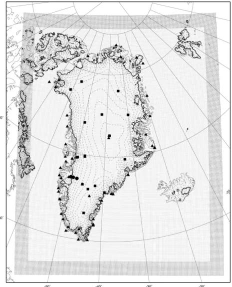
Fig. 1. Map of Greenland featuring the model domain, relaxation

borders (the outer 16 grid points represented as dark gray dots), lo-cation of model grid points (light gray dots) and lolo-cation of observa-tional sites. The 51 DMI climate stations are indicated by triangles, the 15 GC-net automatic weather stations by squares and the three K-transect AWSs by circles. Thin dashed lines are 250 m elevation contours from Bamber et al. (2001). The thick black line represents the ice sheet contour as used in RACMO2/GR.

is 240/360 s depending on the maximum wind speed in the domain, to ensure numerical stability. The 51-year simula-tion took approximately 100 days to run on 60 processors of the ECMWF supercomputer.

RACMO2 has 40 atmospheric hybrid-levels in the vertical, of which the lowest is about 10 m above the surface. Hybrid levels follow the topography close to the surface and pressure levels at higher altitudes. The air temperature and humidity at a standard observational height (2 m above the surface) are computed using an interpolation technique based on the sim-ilarity theory applied to the lowest atmospheric model layers (e.g. Dyer, 1974).

(3)

and ice mask from the digital elevation model of Bamber et al. (2001) are used, which are kept constant during the model simulation. The model surface area of the ice sheet is 1.711×106km2, excluding peripheral ice caps (Fig. 1). This is 1% more than previous studies (Box et al., 2006; Fettweis, 2007; Hanna et al., 2008). Sources of uncertainty include the treatment of changing shelf ice and compacted multi-year sea ice area. The underlying vegetation map is based on the ECOCLIMAP dataset (Masson et al., 2003) and has been manually corrected; the original dataset showed too little tun-dra and too much bare soil along the east coast of Greenland. 2.1 Atmospheric model adjustments

General adjustments to the original dynamical and physical schemes in RACMO2 are described in detail by Van Meij-gaard et al. (2008). Here we only describe the adjustments to the original model formulation that have been made to better represent the melting snow conditions in the Arctic region (RACMO2/GR).

RACMO2/GR calculates the surface turbulent heat fluxes from Monin-Obukhov similarity theory using transfer coef-ficients based on the Louis (1979) expressions. An effective surface roughness length is used to account for the effect of small scale surface elements on turbulent transport. Orig-inally, the roughness lengths for momentum, heat and hu-midity (z0m,z0h,z0q) included the effect of enclosing

veg-etation, urbanization and orography. This approach gave too large values over the Antarctic ice sheet (Reijmer et al., 2004). Therefore, we limitedz0mto 100 mm for tundra

with-out snow and to 1 mm for snow-covered tundra. The value forz0m at the snow covered ice sheet is set to 1 mm, while

z0m is set to 5 mm if bare glacier ice is at the surface. The

roughness lengths for heat and humidity over snow surfaces are computed according to Andreas (1987). Based on his theory, ln(z0h/z0m)or ln(z0q/z0m)are calculated as a

func-tion of the roughness Reynolds number,R∗=u∗z0/υ, where

u∗is the friction velocity,z0the roughness length andυ the kinematic viscosity of air.

Simulations with RACMO2 for the Antarctic region have shown that the original model configuration overestimates liquid precipitation at the expense of solid precipitation (Van de Berg et al., 2006). We imposed that clouds with temper-atures below−7◦C form snow only, so that the solid pre-cipitation flux increases, leaving the total prepre-cipitation sum unchanged. Due to the much lower air temperatures at the higher elevations, this correction only affects the lowest ar-eas of the ice sheet.

2.2 Snow model

The original ECMWF surface scheme (TESSEL; Tiled ECMWF Surface Scheme for Exchanges over Land) does not make a distinction between the snow cover on an ice sheet and seasonal snow cover on the tundra. In TESSEL, snow

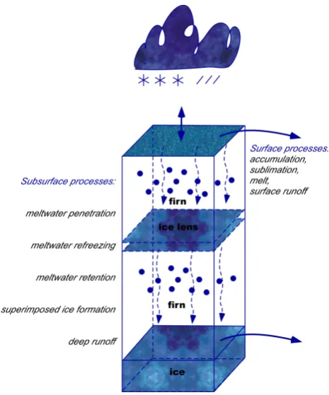
Fig. 2. Schematic representation of modelled processes that

de-termine the surface mass balance. Upper and lower blue surfaces denotes snow-air and snow-ice interfaces, respectively.

cover is treated as a single layer on top of the soil or vege-tation, which is in thermal contact with the underlying soil. This is acceptable for a transient snow layer over the tundra, but not for the semi-permanent ice sheet firn layer. Snow/firn processes such as meltwater percolation, retention and re-freezing are not included, while these are especially impor-tant to realistically simulate the SMB of an ice sheet with ex-tensive summertime melting and refreezing (Genthon, 2001). For a better representation of the processes affecting the SMB in RACMO2/GR, we introduced an additional sur-face tile “ice sheet” in the land sursur-face scheme TESSEL to describe the interaction at the snow/firn/ice-atmosphere in-terface (Fig. 2). As the ice temperature at the bottom of the ice/firn/snow pack is kept constant, no heat flux is as-sumed through the lower boundary. The subsurface pro-cesses are parameterized for at least the upper 30 m with a multi-layer snow/firn/ice model (1-D) composed of a maxi-mum of 100 layers, but of 40 layers on average. The melt-water formed at the surface is allowed to penetrate to deeper layers, where it may refreeze (internal accumulation) or runs off as described by Bougamont et al. (2005).

(4)

vertical grid is adjusted by layer splitting when the layer thickness becomes more than 1.3 times its optimal thickness, or layer fusion when a layer is less than half of its optimal thickness, except for layers consisting of ice lenses in the firn.

Snow/firn densityρcontinually changes in time due to re-freezing of capillary water (rain and meltwater) and the set-tling and packing of dry snow according to the empirical for-mulation by Herron and Langway (1980):

forρ < 550 kg m−3: dρ

dt =k0a (ρi−ρ) (1)

withk0=11exp

−10 160

RT

for 550 kg m−3 ≤ρ < 800 kg m−3: (2) dρ

dt =k1a

0.5_(ρ

i−ρ)

withk1=575exp

−21 400

RT

whereais the annual mean accumulation rate,Rthe univer-sal gas constant andT the firn/snow temperature in K. The annual accumulation rate used in this formula is the spatially distributed accumulation averaged over the period 1989– 2005 based on a 16-year integration with RACMO2/GR.

The snow/firn/ice column is thermally coupled to the at-mospheric part of RACMO2/GR through a surface skin layer formulation of the surface energy balance (SEB) and the sur-face albedo,α, which is also applicable to the other surface tiles, such as tundra, sea-ice and open ocean. The skin tem-perature is introduced for modelling purposes and is defined as the temperature of the skin layer at the surface-atmosphere interface that is infinitely thin, has no heat capacity and re-sponds instantaneously to SEB changes. The skin tempera-tureTsis solved by SEB closure (e.g. Brutsaert, 1982):

M =SWnet+LWnet+LHF+SHF+Gs

=SW↓(1−α)+LW↓−σ T_s4+LHF+SHF+Gs (3) where M is the melt energy, SWnet, SW↓, SW↑, LWnet, LW↓, LW↑ the net, downward and upward directed fluxes

of shortwave and longwave radiation,αthe broadband sur-face albedo,the surface emissivity for longwave radiation (=0.98 in RACMO2/GR for the ice sheet),σ the Stefan-Boltzmann’s constant, LHF and SHF the turbulent fluxes for latent and sensible heat and Gs the subsurface conductive heat flux evaluated at the surface. All terms are defined as positive when directed towards the surface-atmosphere inter-face.

The skin temperature serves as a boundary condition to the englacial module, which treats the vertical conduction of heat as follows:

ρ cp

∂T

∂t = −

∂ ∂z

k∂T

∂z

+Q= +∂G

∂z +Q (4)

whereρis the density of the snow/firn/ice layer,cpthe spe-cific heat capacity of ice (2009 J kg−1_K−1_),_∂T_/_∂t_{the rate of} temperature change within one model time step,kthe effec-tive conductivity,zthe vertical coordinate andQthe heat re-leased by refreezing of meltwater. The term∂G/∂zaccounts for the heat diffusion driven by the vertical temperature gra-dient. The snow/firn/ice conductivity follows the density-dependent approach of Van Dusen (1929), which ensures the correct value for k if ice density is attained. Temperature dependence ofkis neglected:

k=2.1×10−2+4.2×10−4ρ+2.2×10−9ρ3 (5) Knowing the conductivity of the snow/firn/ice layers, the ver-tical snow/ice temperature profiles can be computed. IfTsis larger than 0◦_{C, it is reset to the melting point of ice and the}

excess of energy is used for melting. Meltwater and rain are allowed to percolate into the firn until they refreeze or run off. The maximum retention capacity due to capillary forces is set to a low value of 2% of available pore space, to obtain a realistic densification rate by refreezing of capillary water (Greuell and Konzelman, 1994). If an ice surface is encoun-tered, the remaining water runs off at the surface, or deep in the firn pack at the snow/ice transition, without delay.

The snow/firn/ice albedo α follows the snow density (ρ) and cloudiness (n) dependent linear formulation of Greuell and Konzelman (1994) for the uppermost 5 cm of the snow/firn/ice pack.

α=αi+(ρ1−ρi)

(αs−αi)

(ρs−ρi)

+0.05(n−0.5) (6) where the subscript i denotes ice and subscript s denotes snow. This parameterization is based on the notion that den-sity reflects the metamorphosis state of the snow, i.e., it rep-resents mostly the effects of grain size on albedo. Fresh snow is characterised by a surfaceαof 0.825 and a density of 300 kg m−3. Glacier ice has an albedo of 0.5 and a den-sity of 900 kg m−3_{. Refrozen meltwater or rain may increase} the density of the firn pack to the ice density, but the sur-face albedo is limited to a minimum value of 0.7 for refrozen water (Stroeve et al., 2005). This limitation will mainly af-fect areas south of 70◦N, where daytime melt and nighttime refreezing occur regularly throughout the melt season. 2.3 Model initialization

(5)

In the dry-snow zone, where melting is rare, the mean air temperature is a reasonable approximation (within 2◦_{C) for}

the climatological deep snow and ice temperature. For this reason, the snow/firn/ice temperature is initialized vertically uniform with the climatological surface temperature as de-scribed by the empiral function of Reeh (1991), who pre-sented a snow/ice temperature parameterization as a func-tion of elevafunc-tion and latitude based on air temperature data from Danish meteorological stations at the periphery of the ice sheet for the 1951–1961 period:

T = T2 m +δT (7)

with T2 m = 48.83 −0.007924z−0.7512φ

δT = 0.86+26.6(SIF− 0.038)

whereT is the climatological ice temperature in ◦C, T2 m the 2 m air temperature in ◦C that depends on elevation z

in m and latitudeφin◦N, andδ T a perturbation due to the amount of superimposed ice formed, SIF. For SIF, the melt rate is averaged over the period 1989–2005 based on a 16-year integration of RACMO2. For the percolation and ab-lation zones, a temperature correctionδ T due to refreezing energy is included in line with Reeh (1991), and the ice tem-perature is limited to 0◦C. The resulting deep ice temperature serves as a boundary condition for the lowest firn/ice layer, so no heat flux is allowed in the underlying ice or soil.

For the 51-year model simulation, the initial temperature and density profiles of the snow/firn/ice column were ob-tained by rerunning the first model year (1 September 1957 to 31 August 1958) three times to reduce spin-off effects. Analysis of the three spin-up years and the first years of the simulations shows that the initial snow pack is in a state of near-balance before the present-day climate run is started.

3 Observational data

A proper assessment of RACMO2/GR output is essential be-fore its data can be used as a tool for studying the climate of Greenland and the recent changes. Moreover, identification of model deficiencies may help to improve the model formu-lation for future climate simuformu-lations. To verify the model results for the surface conditions, we use: (i) near-surface air temperature and wind speed data from automatic weather stations (AWSs) on the ice sheet (GC-net; Steffen and Box, 2001 and K-transect; Oerlemans and Vugts, 1993) and from climate stations of the Danish Meteorological In-stitute (DMI) on the surrounding tundra, (ii) data of surface radiation and heat exchange processes from three K-transect AWSs (Van den Broeke et al., 2008a,b).

Statistical procedures were applied to all observational datasets to remove occasional spurious data values. For model evaluation of monthly means, we require that at least

80% of the observations are available during one month. The length of an observational record does not influence the evaluation, since every separate month is compared indepen-dently with the same month from the model output. The el-evation of model grid points closest to all observational sites is within 100 m of the observed elevation, suggesting that no height correction is needed for temperature.

3.1 GC-net

The Greenland Climate Network (GC-net) was started in 1995 and consisted of 15 AWSs until 2001 (indicated as squares in Fig. 1) near or above the 2000 m elevation contour. Station coordinates and detailed information on the measure-ments are given in Steffen and Box (2001). We obtained a complete and quality controlled dataset for the period 1998– 2001. For this period, the biases were removed and neces-sary corrections were applied. As the quality of the observa-tions for the more recent years could not be guaranteed, this dataset nor the dataset from the DMI stations, are extended.

Four parameters derived from direct observations are com-pared with the RACMO2/GR output: 2 m air temperature, 10 m wind speed, net shortwave radiation and net radiation, as they are described by Box and Rinke (2003). The air tem-perature at 2 m is calculated by using the observed tempera-tures at 2 levels, heights of the instruments (median heights are 1.4 and 2.6 m) and linear interpolation. A logarithmic wind profile with a roughness length of 0.5 mm is assumed to estimate the 10 m wind speed. Due to riming of the sensors, net shortwave radiation data are omitted for the springtime months March and April. Most of the available net radiation observations are excluded in this study, because these unven-tilated measurements often suffer from large errors due to riming inside and outside the polyethylene domes. Only the net radiation records of the sites Swiss Camp and JAR1 are believed to be reliable throughout the year.

3.1.1 K-transect

As part of GC-net, UU/IMAU installed three AWSs along the Kangerlussuaq transect (K-transect) in southwest Green-land in August 2003 (Van den Broeke et al., 2008b,c) (indi-cated as circles in Fig. 1). Measurements have been com-pared to model output for the period August 2003 to August 2007. The AWSs at S5 (490 m a.s.l.), S6 (1020 m a.s.l.) and S9 (1520 m a.s.l.) are located in the ablation and percola-tion zone (Fig. 3). The surface at S5 is very irregular with 2–3 m high ice hummocks usually covered with a thin layer of drift snow during wintertime, while at S9 the surface is much smoother, covered by a layer of wet snow for most or all of the summer. The changing surface conditions through-out the year make this dataset valuable for a thorough model evaluation on a daily basis.

(6)

Fig. 3. Images of the AWSs along the K-transect and their

sur-roundings at S5, S6 and S9. Images taken at the end of the ablation season (end of August). Photos by Paul Smeets (UU/IMAU).

assess the model performance for the seasonal cycle. The comparison of daily values is focused on the year 2004, an average year within the 51-year simulation.

The accuracy of the measured temperature and wind speed at approximately 2 and 6 m is 0.3◦C and 0.3 m s−1, respec-tively, as stated by Van den Broeke et al. (2008c). As the transformation to the 2 m temperature is only done when both measurements were available and by applying the bulk method, errors in the transformation are small. Further in-formation on the sensor specifications and data quality is de-scribed in Van den Broeke et al. (2008a).

The observed surface radiation balance, surface charac-teristics, cloud properties and surface energy fluxes are de-rived from the AWS data with a melt model as described by Van den Broeke et al. (2008a,b). The observed (corrected) net shortwave radiation and the incoming longwave radiation fluxes serve as direct input for this melt model. The measure-ments of wind speed, temperature and humidity at two levels (approx. 2 and 6 m) serve as input for the bulk method to cal-culate the sensible and latent turbulent heat fluxes (Deardorff, 1968; Van den Broeke, 1996).

3.2 DMI climate stations

DMI climate stations are operated around the Greenland pe-riphery (indicated as triangles in Fig. 1) and provide daily records of wind speed, air temperature and precipitation (Cappelen et al., 2001). For the model evaluation we used the dataset as described by Yang et al. (2005), which com-prises of measurements during the period 1 January 1973 to 1 February 2005. Data from 51 stations is compared with model output for the nearest grid point that is considered as land in RACMO2/GR. As a result, some stations on small islands or narrow peninsulas are excluded from the analyses. Model evaluation is limited to annual and climatological means because of the inability of the 11 km model grid to resolve local complex terrain surrounding the land stations. We computed monthly means of the wind speed and temper-ature, and averaged them over a year or over the measuring period to obtain an annual mean or climatological value for each site for comparison with RACMO2/GR output.

4 Model evaluation

The comparison of model values that represent averages for a model grid cell with a typical area of 121 km2, with local point observations must be done carefully. The model grid box closest to the observational site does not necessarily have the same surface type, elevation, surface roughness or surface albedo. In the interior of the ice sheet, these discrepancies are smaller since the surface is more homogeneous and the climate gradients less steep.

(7)

4.1 Temperature at 2 m

The near-surface or 2 m temperature (T2 m) is an important climate variable, and one of the primary variables used in climate change reports as it is measured at many sites across the globe. Moreover, the near-surface saturation specific hu-midity, and consequently also sublimation/deposition at the surface, all strongly depend on the near-surface temperature. Typical for the interior of the ice sheet is a surface tempera-ture inversion, driven by surface radiative cooling and in part compensated by the downward (air-to-surface) transport of sensible heat (SHF). This temperature deficit drives a persis-tent katabatic wind circulation over the ice sheet (Steffen and Box, 2001).

Figure 4a shows that for the entire ice sheet (green and red dots) and the surrounding tundra (black dots), the simulated climatological values ofT2 mare in close agreement with the observations(R=0.97)with an averaged bias of−0.8◦C. The model tends to slightly underestimate/overestimate the near-surface temperature on the tundra/ice sheet. The aver-aged land bias is−1.5◦C (R=0.96), whereas the ice sheet bias is +0.9◦C (R=0.99). Only at some of the locations along the coastline of Greenland, does RACMO2/GR devi-ate more than 4◦C from the observations. The largest model bias (−9.8◦C) is found for DMI station 43800, located along the southeast coast near Tingmiarmiut. Disregarding this sta-tion reduces the root mean square error (RMSE) of 2.3◦_{C to}

2.0◦_{C when taking all locations into account, and from 2.1}

to 1.7◦_{C for only the land sites.}

The temperature bias is uncorrelated to the elevation bias and does not show coherent regional patterns because of the irregular distribution of the stations over Greenland, but seems to be correlated to the land surface type. In RACMO2/GR, tundra and ice sheet are considered as differ-ent surface tiles with specific characteristics, such as albedo, thermal skin conductivity and vegetation type. The calcula-tion of the surface fluxes is done separately for these different surfaces, leading to different solutions for the SEB equation and skin temperature even if the overlying atmosphere would be identical. A similar inland warm bias has been identified in ERA-40 data (Hanna et al., 2005), in part ascribed to posi-tive bias in downward longwave radiation from the Rapid Ra-diative Transfer Model (RRTM) scheme, which is also used in RACMO2/GR.

Figure 5 shows the observed and modelled 2 m tempera-ture deviations from their annual mean value (1973–2004) for 4 long-term DMI stations at various locations around the ice sheet. The model closely follows the observed tempera-ture over the measurement period, also over the most recent years when warming has been reported Hanna et al. (2008); Box et al. (2009). Comparison of the long-term measure-ments at all climate stations with the model output indicates that the land bias (ranging from−4.4 to 0.8◦C) is stable in time, so that the interannual variability is well captured by RACMO2/GR. The standard deviation of the observations is

-35 -30 -25 -20 -15 -10 -5 0 5

GC net DMI

K-transect

Modelled 2 m temperature [

o C]

Observed 2 m temperature [oC]

(a)

-6 -5 -4 -3 -2 -1 0 1 2 3

1 2 3 4 5 6 7 8 9 10 11 12

S5

S6 S9

2 m temperature [

o C]

month

(b)

Fig. 4. Model performance for 2 m temperature [◦C]. (a) model versus observations for GC-net (black), DMI coastal stations (red), and K-transect (green), averaged over the available measuring pe-riod, (b) monthly model bias (2003–2007) along the K-transect for S5 (black), S6 (red) and S9 (blue).

for 3 out of 4 shown stations larger than the modelled stan-dard deviation, which is valid for the whole climate stations dataset. This points towards a systematic underestimation of the interannual variability by RACMO2/GR for the land sta-tions, rather than an increasing model drift due to incorrect initializations.

(8)

-3 -2 -1 0 1 2 3

1975 1980 1985 1990 1995 2000 2005

Observed Modeled T2m a n o ma ly [K] Year (a) -3 -2 -1 0 1 2 3

1975 1980 1985 1990 1995 2000 2005

Observed Modeled T 2m a n o ma ly [K] Year (b) -4 -3 -2 -1 0 1 2 3

1975 1980 1985 1990 1995 2000 2005

Observed Modeled T2m a n o ma ly [K] Year (c) -3 -2 -1 0 1 2 3

1975 1980 1985 1990 1995 2000 2005

Observed Modeled T 2m a n o ma ly [K] Year (d)

Fig. 5. Comparison of simulated (dashed lines) and observed (solid

lines) annual mean 2 m temperature anomaly [K] with respect to their mean value (1973–2004) for 4 DMI climate stations at (a) Thule, (b) Tasiilaq, (c) Sondre Stromfjord, and (d) Julianehavn.

Table 1. Comparison between seasonal and annual modelled and

observed 2 m temperature [◦C] for the stations S5, S6 and S9 along the K-transect. The bias is calculated between the modelled and ob-served data, the standard deviation (Std) is based on daily obob-served data over the period August 2003–August 2007.

S5 S6 S9

Bias Std Bias Std Bias Std

DJF −4.1 7.8 0.8 8.3 −0.2 8.4

MAM −2.3 8.2 0.9 8.5 0.9 8.4

JJA −1.2 1.7 0.7 1.8 0.7 2.6

SON −2.8 6.6 0.9 7.3 0.5 7.7

Annual −2.6 9.3 1.1 9.8 0.5 10.2

For two sites along the K-transect, S6 and S9, the mean monthly bias is 1.1 and 0.5◦C and the RMSE 0.5 and 0.7◦C, respectively. These biases and RMSE are consider-able smaller than one standard deviation, which indicates that RACMO2/GR is capable of simulating the temporal variabil-ity. The warm bias is stable through the year (Table 1), except

-40 -30 -20 -10 0 10

Jan/1 Feb/1 Mar/1 Apr/1 May/1 Jun/1 Jul/1 Aug/1 Sep/1 Oct/1 Nov/1 Dec/1 Jan/1

2 m temperature [

oC] Date (a) 0 5 10 15 20

Wind speed [m s

-1] Date (b) 0.65 0.7 0.75 0.8 0.85 0.9 0.95 1

2004/1 2004/7 2005/1 2005/7 2006/1 2006/7 2007/1 2007/7

Directional constancy [-]

Date (c)

Fig. 6. Comparison of simulated (gray lines) and observed (black

lines) daily averaged (a) 2 m temperature [◦C], (b) 10 m wind speed [m s−1] at S6 for the year 2004, and (c) comparison of simulated (gray lines) and observed (black lines) monthly averaged directional constancy [−] of 10 m wind at S6 for the period January 2004– August 2007.

for winter (DJF) at S9 (−0.2◦C), indicating that the seasonal cycle is well captured. A similar realistic seasonal cycle in

T2 m is found for the low-elevation sites of GC-net, Swiss Camp and JAR1 (not shown).

On a daily basis, Fig. 6a shows that for site S6 the differ-ence between the observed values and RACMO2/GR is gen-erally low for the year 2004 (RMSE=1.9◦C). The model follows the observed temporal evolution closely throughout the year. The large day-to-day fluctuations of over 10◦C dur-ing the winter are well represented in the model output, indi-cating that RACMO2/GR is capable of simulating the vari-ability in weather and the related changing atmospheric con-ditions over the ice sheet. The largest model biases are found in the transition months April and September, which is asso-ciated with an underestimation of the surface albedo leading to more net shortwave radiation absorption (see Sect. 4.4.1). Similar results are found for the other years.

(9)

is located at only 6 km from the ice sheet margin on an ice tongue (Russell Glacier) that protrudes from the ice sheet onto the tundra. Its closest model grid point is classified as ice sheet, while some of its neighbouring grid points are clas-sified as tundra. The 1◦C summer cold bias at S5 may be caused by too much nocturnal cooling of the surface in the model, whereas the ice surface is observed to be at melting point day and night. In winter, it is well known that temper-atures over flat tundra are considerably lower than over the adjacent ice sheet, where katabatic winds prevent the forma-tion of a strong temperature inversion (e.g. Van den Broeke et al., 1994). Therefore, winter temperature biases at S5 are thought to result from insufficient downward longwave radi-ation and/or overestimradi-ation of cold air pooling over the tun-dra.

4.2 Wind speed and direction at 10 m

To assess the model performance for wind over the whole ice sheet, we compare RACMO2/GR with in situ observa-tions averaged over matching time periods (Fig. 7a). Both low and high wind speeds are well represented with a mean difference of only 0.3 m s−1(RMSE=1.9 m s−1). This sug-gests that the surface friction is adequately accounted for in the model and that the vertical resolution of the model with its lowest layer at about 10 m above the surface is sufficient for simulating the near-surface katabatic wind profile, as found by Reijmer et al. (2005) for Antarctica. The monthly mean observed standard deviation (2.9 m s−1) is consider-ably larger than the mean bias and RSME, which implies that RACMO2/GR is capable of simulating the near-surface wind speed variability.

The correlation between the model output and the observa-tions is high (R=0.74), considering that the measured wind speed may be affected by local topography. Furthermore, a considerable uncertainty exists in both the in situ and model wind speed at 10 m owing to poorly defined stability correc-tions in very stable surface layers, which regularly occur over the interior of the ice sheet. In situ sensors also occasion-ally accumulate rime, which could be expected to introduce a negative wind bias. Because the AWSs are un-attended, it is impossible to quantify how large this error is.

The seasonal cycle of wind speed is largely controlled by the strength of the katabatic forcing, which is largest in win-ter (Van de Wal et al., 2005). Along the K-transect, the surface is considerably smoother at S9 than at S5 and S6 (Fig. 3). As a result the strongest seasonal cycle is found at S9 with monthly averaged summer wind speeds of 6 m s−1 and 11 m s−1during February. Averaged over the K-transect, the modelled 10 m monthly wind speed deviates less than 1 m s−1 from the observations (Fig. 7b). Similar results are found for the different seasons. At S5 and S9 the av-eraged seasonal bias is uniform over the year and slightly negative (−0.4 and−0.3 m s−1, respectively), but consider-ably smaller than the observed standard deviation (2.5 and

0 2 4 6 8 10

GC net DMI K-transect

Modelled 10 m wind speed [m s

-1 ]

Observed 10 m wind speed [m s-1]

(a)

-3 -2 -1 0 1 2

1 2 3 4 5 6 7 8 9 10 11 12

S5 S6 S9

10 meter wind speed [m s

-1 ]

month (b)

Fig. 7. Model performance for 10 m wind speed [m s−1]. (a) model versus observations for GC-net (black), DMI coastal stations (red), and K-transect (green), averaged over the available measuring pe-riod, (b) monthly model bias for S5 (black), S6 (red) and S9 (blue) over the period August 2003–August 2007.

3.1 m s−1). At S6 the seasonal biases are close to zero, except for summer (bias=0.7 m s−1), probably due to an inaccurate transition of snow to bare ice (see Sect. 4.4.1). At these lower elevations, the estimates of 10 m wind speed based on sim-ilarity theory may be more reliable, because enhanced tur-bulent mixing due to increasing wind speeds minimizes the stability effects.

(10)

wind speed events, possibly due to a too low modelled sur-face roughness. A remarkable feature is the daily averaged wind speed, which is always above 1 m s−1_{apart from a short} period during which the sensor was frozen. This is because a continuous surface temperature inversion develops owing to negative net surface radiation in winter and a surface tem-perature restricted to the melting point in summer, causing a persistent katabatic wind throughout the year over the slop-ing surface of the ice sheet.

The wind regime on the ice sheet is dominated by semi-permanent katabatic winds (Steffen and Box, 2001). Kata-batic winds are characterised by (a) a maximum in wind speed close to the surface and (b) a constant wind direction. The directional constancy dc is a useful tool to detect lo-cal persistent circulations and is defined as the ratio of the vector-averaged wind speed to the mean wind speed usually taken at 10 m (Bromwich, 1989):

dc = u

2 ₊_v21₂

u2 +v2

1 2

(8)

whereu and v are the horizontal components of the 10 m wind. A dc of zero implies that the near-surface wind di-rection is random. When dc approaches 1, the wind blows increasingly from the same direction. Close to the ice mar-gin, the directional constancy and wind speed peak twice a year. In winter, the katabatic wind forcing is maintained by the radiation deficit at the surface, whereas in summer, the snow/ice at the surface melts and prevents the surface tem-perature from rising above melting point, so that katabatic winds persist. For S6, RACMO2/GR underestimates the per-sistence of the katabatic flow by∼5% on average (Fig. 6c), but the double annual maximum is well (R=0.9) repre-sented.

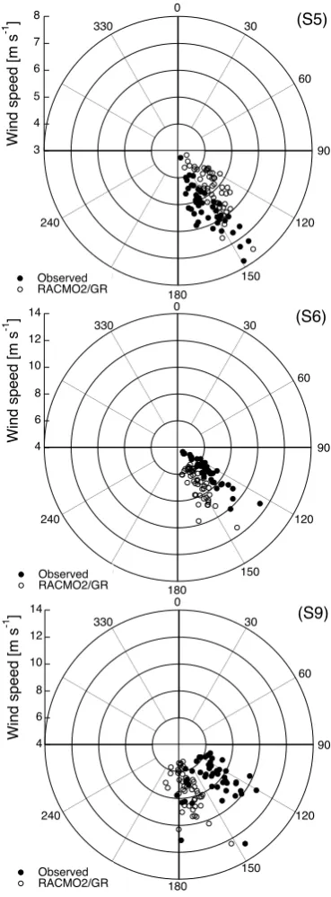
The mean wind direction along the K-transect is south-southeasterly (Fig. 8). This dominant wind direction is de-termined by storms and the persistent katabatic flow that is deflected to the right of the downslope direction due to the Coriolis force. A downslope (cross-isobar) component is maintained by friction. The wind direction is well simulated by RACMO2/GR, although it is too strongly (26 degrees on monthly basis) deflected at S9, possibly due to an underesti-mated surface roughness length.

4.3 Humidity at 2 m

The near-surface specific humidity is strongly controlled by air temperature. Along the K-transect, higher elevated sites have lower average specific humidity, modelled and ob-served. When specific humidity is high, temperatures are also high and visa versa, which follows the essential Clau-sius Clapeyron function.

Figure 9a, shows that at S6, the agreement between the daily RACMO2/GR values and observations of spe-cific humidity is good (R =0.98), both for the very

3 4 5 6 7

8 0

30

60

90

120

150 180

210 240

330

Observed RACMO2/GR

Wind speed [m s

-1 ] (S5)

4 6 8 10 12

14 0

30

60

90

120

150 180

210 240

330

Observed RACMO2/GR

Wind speed [m s

-1 ] (S6)

4 6 8 10 12

14 0

30

60

90

120

150 180

210 240

330

Observed RACMO2/GR

Wind speed [m s

-1 ] (S9)

Fig. 8. Comparison of simulated (open circles) and observed (solid

circles) monthly averaged 10 m wind direction and speed at S5, S6 and S9 for the measurement period August 2004–August 2007.

(11)

0 1 2 3 4 5

Specific humidity [g kg

-1 ]

Date

(a)

40 50 60 70 80 90 100

Relative humidity [%]

Date (b)

Fig. 9. Comparison of simulated (gray lines) and observed (black lines) 2 m daily averages of (a) specific humidity [g kg−1] and (b) relative humidity [%] at S6 for the year 2004.

observations closely (Fig. 9a). The observed and modelled standard deviations are identical (1.42 g kg−1_{), and} consider-ably larger than the above-mentioned bias and RMSE. At S9, the bias and RMSE are even smaller (bias= −0.005 g kg−1; RMSE=0.27 g kg−1). For S5, RACMO2/GR performs slightly worse (bias= −0.25 g kg−1; RMSE=0.35 g kg−1). This bias is also persistent throughout the year.

When analysing the 2 m relative humidity RH2 m, it ap-peared that in the standard post-processing of RACMO2 data, the latent heat of vapourization is used for the compu-tation of the saturated vapour pressure as prescribed by the WMO (World Meteorological Organization), whereas sub-limation/deposition takes place at freezing winter tempera-tures. Since the observed RH2 m is derived using the latent heat of sublimation, RACMO2/GR would significantly un-derestimate RH2 m by−14.4%. Therefore, we recomputed modelled RH2 m using the daily specific humidity model values and the latent heat of sublimation, which reduced the mean daily bias to −7.2%. The observed RH2 m at S6 remains close to saturation throughout the year, while RACMO2/GR shows an unexpected decrease in wintertime (Fig. 9b). This discrepancy is also found for the observa-tional years 2005 and 2006. In summer, both observed and modelled RH2 m decrease towards the lower elevations (not shown). A possible explanation is that the katabatic wind transports colder, dry air downwards and that adiabatic com-pression and the associated heating results in a lower relative humidity downslope in summer. Measurement uncertainties at low temperatures are also a possible explanation.

4.4 Surface energy balance

The air temperature near the surface is strongly coupled to the surface temperatureTs, which is determined by the sur-face energy balance (SEB). The SEB (Eq. 3) voor the GrIS is largely controlled by the radiative fluxes and the surface albedo, and to a lesser extent by the turbulent fluxes and the subsurface heat flux (Van den Broeke et al., 2008b,a). The performance of RACMO2/GR for different terms in the SEB will be discussed in this order. Few reliable measurements of SEB components on the ice sheet are available. We rely on SEB observations along the K-transect, where the AWSs are equipped with K&Z CNR1 radiation sensors that measure all four radiation components individually.

4.4.1 Net shortwave radiation and surface albedo

The SEB is strongly influenced by net shortwave radiation that is absorbed at the surface and which drives a clear seasonal and diurnal cycle unless the energy is used for melting. Along the K-transect, the model bias in SW↓ is

time-dependent. While RACMO2/GR estimates SW↓to be

(12)

each of these processes separately cannot be clarified without detailed cloud-radiation observations and modelling.

The reflected shortwave radiation depends on the amount of incident shortwave radiation at the surface and the sur-face albedo. The latter is observed to be asymmetric through the year in the ablation zone (Van den Broeke et al., 2008a). Comparing daily model output with the K-transect obser-vations reveals a too early decrease and a too late increase in modelledα, ranging from only a few days up to weeks (Fig. 10) for all evaluated years. In early summer, the winter snow pack melts, leading to a transition from a dry snow pack (modelledαof 0.825) to a wet snow pack with modelledαof

≈0.7, followed by the appearance of the underlying glacier ice with modelledαof≈0.5. The rate of this transition pro-cess is hard for RACMO2/GR to capture, since the modelled surface albedo is determined based on the density of the up-per 5 cm of dry snow, unaffected by the presence of water in the snow pack. Furthermore, in reality, some redistribution of falling snow by the wind occurs (Van den Broeke et al., 2008a). The radiation sensor is mounted on the AWSs that stands on top of an ice hummock (Fig. 3) and, thus, there is a likely sampling bias toward lower albedo, especially in the early melt season.

The observed daily variations inαassociated with snow-fall events are underestimated by the model (Fig. 10). In the observations,αrises more abruptly during a snowfall event, even if only a very thin layer of fresh snow covers the sur-face. In the model, αresponds only to significant changes in the density of the upper 5 cm of the snow/firn/ice pack, which requires a more substantial snowfall event. The same discrepancy between model and observations is responsible for the late increase in modelαduring autumn, as fresh snow starts to cover the glacier ice. Similar systematic biases are found for the other years of the measurement period. The timing of the spring melt and of the fresh snowfall in autumn does change for the different years, but the time lag between the model and observations is similar (not shown). Over-all, the surface albedo evolution through all four summers (2004–2007) is captured reasonably well (quantified below) by RACMO2/GR (R=0.73), taking into account that the ab-lation zone is characterised by a very inhomogeneous sur-face.

The underestimation of the albedo in early summer and autumn leads, on average, to a positive model bias in the re-flected shortwave radiation of +9 W m−2averaged over the K-transect (not shown). In the ablation zone, the positive bi-ases in the reflected shortwave radiation lead to an overesti-mation in the net shortwave radiation, with the largest biases in the spring and summer months (Fig. 11b and Table 2). Figure 12a shows that RACMO2/GR significantly overesti-mates SWnetat S6 by 31% in summer compared to the obser-vations. As expected, the bias in SWnet is smaller for most of the dry snow zone (GC-net stations in Fig. 11a), where the surface albedo remains relatively high and constant through-out the year. Only a significant deviation from the assumed

0.4 0.5 0.6 0.7 0.8 0.9 1

Apr/1 May/1 Jun/1 Jul/1 Aug/1 Sep/1 Oct/1

Albedo [-]

Date (S5)

0.4 0.5 0.6 0.7 0.8 0.9 1

Albedo [-]

Date (S6)

0.4 0.5 0.6 0.7 0.8 0.9 1

Albedo [-]

Date (S9)

Fig. 10. Time evolution of the daily surface albedo [−] in the ob-servations (black lines) and model output (gray lines) for the three AWSs (S5, S6 and S9) along the K-transect for the period April– October 2004.

fresh snowαof 0.85 may result in an overestimation at the accumulation zone sites.

4.4.2 Net longwave radiation

At S6, the daily variation in net longwave radiation LWnet is well captured by RACMO2/GR (Fig. 12b). The model tends to underestimate the lower range of values during the winter months (Table 2). This negative bias is caused by an underestimation of LW↓, with as largest bias −30 W m−2.

Van de Berg et al. (2007) encountered a similar problem over the Antarctic ice sheet using an earlier version of RACMO2, which they related to an underestimation of the clear-sky ra-diance, winter cloud cover and humidity. Similarly to biases in SW↓, detailed cloud observations are needed to quantify

the effect of a potential bias in cloud properties on LW↓.

At S6, the resulting winter negative bias in LWnet is 16 W m−2 _{(Table 2), whereas the monthly average bias in} LW↑is only±5 W m−2(Fig. 13a). In summer, the LW↑bias

diminishes as the melting surface limits the surface tempera-ture. For S9, the performance of RACMO2/GR is similar to S6. For S5 however, the cold bias (see Fig. 4b) results in an underestimation of LW↑in winter of 25 W m−2,

(13)

10 15 20 25 30 35 40 45 50

K-transect GC net

Mo

d

e

lle

d

n

e

t

sh

o

rt

w

a

ve

ra

d

ia

tio

n

[

W

m

-2 ]

Observed net shortwave radiation [W m-2] (a)

-20 -10 0 10 20 30 40 50 60

1 2 3 4 5 6 7 8 9 10 11 12

S5 S6 S9

N

e

t

sh

o

rt

w

a

ve

ra

d

ia

ti

o

n

[

W

m

-2 ]

month

(b)

Fig. 11. Model performance for surface net shortwave radiation [W m−2] (a) model versus observations for GC-net (black) and K-transect (green) averaged over the available measuring period, (b) monthly model bias for S5 (black), S6 (red) and S9 (blue) over the period August 2003–August 2007.

Table 2. Seasonal and annual bias between the modelled and observed surface energy fluxes [W m−2] for the stations S5, S6 and S9 over the period August 2003–August 2007.

S5 S6 S9

DJF JJA Ann DJF JJA Ann DJF JJA Ann

SWnet −0.2 25.9 8.8 0.6 23.6 10.7 0.6 27.3 9.3

LWin −25.6 −13.6 −18.5 −19.0 −3.1 −9.0 −30.5 −5.6 −14.6

LWnet −2.8 −11.4 −5.0 −15.9 −3.6 −8.7 −23.1 −7.2 −12.9

NetR −2.5 14.5 3.7 −15.3 19.9 2.1 −22.5 20.1 −3.6

SHF 10.3 −4.5 2.6 22.7 20.1 15.9 21.8 4.9 10.5

LHF 3.3 −3.9 1.9 −3.8 −4.3 −4.7 −3.0 −4.0 −3.6

4.4.3 Net radiation

In Fig. 12c, the net result of the daily shortwave and long-wave radiation fluxes is presented for S6. In wintertime, shortwave radiation is reduced to near zero and LWnetdrives the surface radiation budget. The negative bias in LW↓leads

to an underestimation of net radiation and is thought to be the result of underestimated clear sky longwave radiance and/or of cloudiness (see Sect. 4.4.2). In summer, the positive bias in SWnetis the dominant contribution to an overestimation of the net radiation absorbed at the surface. Figure 13b shows that for S6 the largest disagreement is found in spring, when the negative bias in albedo is largest. At S5 and S9, the bias in net radiation is smaller due to a better representation of the surface albedo variability in the summer half year. A similar bias is found for the GC-net sites JAR1 and Swiss Camp that are located in environments comparable to S9 (not shown). The correlation between net radiation observed at 20 ice sheet locations and modelled is 0.79 with climatological mean bias of 2.5 W m−2and RMSE of 3.3 W m−2.

4.4.4 Turbulent heat fluxes

(14)

0 50 100 150 200

SW

net

[W m

-2]

Date (a)

-100 -80 -60 -40 -20 0 20

LW

net

[W m

-2]

Date (b)

-100 -50 0 50 100 150

Net radiation [W m

-2]

Date (c)

Fig. 12. Comparison of simulated (gray lines) and observed (black

lines) daily averaged values of (a) net shortwave radiation flux SWnet, (b) net longwave radiation flux LWnet, and (c) net

radia-tion flux in [W m−2] at S6 for the year 2004. Note the different vertical scales used in the panels.

During the summer, the largest positive bias is found at S6 (about +20 W m−2), while at S5 and S9 the biases (−4.9 and +4.1 W m−2, respectively) are much smaller.

The annual cycle of latent heat flux LHF is of importance to the SEB. Surface temperatures continuously below freez-ing lead to deposition (rime formation) in winter and subli-mation in spring and summer (Fig. 14b). To obtain a realistic sublimation, it is important that at least the surface temper-ature is correctly represented. Differences in LHF between RACMO2/GR and observational sites along the K-transect are less than±5 W m−2in winter months and about 5 W m−2 during summer (Fig. 15b and Table 2). The annual bias is

−2.0 W m−2averaged over these 3 sites. The largest monthly biases are found at S5, coinciding with a largeT2 m bias. It should be noted here that “observed” turbulent fluxes are ap-proximated by the bulk fluxes, which are also somewhat un-certain (Box and Steffen, 2001).

5 Summary and conclusions

An assessment of the performance of RACMO2/GR, a regional climate model with physical parameterizations optimized for use over the extensive ice sheets, is

pre--40 -30 -20 -10 0 10 20

1 2 3 4 5 6 7 8 9 10 11 12

S5 S6 S9

LW

net

[W m

-2 ]

month

(a)

-40 -20 0 20 40 60

1 2 3 4 5 6 7 8 9 10 11 12

S5 S6 S9

Net radiation [W m

-2 ]

month (b)

Fig. 13. Model performance for (a) the net longwave radiation and (b) the net radiation for S5 (black), S6 (red) and S9 (blue) along the

K-transect in [W m−2] over the period August 2003–August 2007.

sented using in situ observations on and around the Green-land ice sheet. This analysis has primarily focused on the near-surface atmospheric state (temperature, humidity, wind speed and direction), and the surface energy balance compo-nents including the radiative fluxes.

We found a good correlation (bias= −0.8◦C,R=0.97, RMSE=2.3◦C) between modelled and measured climato-logical value ofT2 mat 70 stations across the ice sheet. The temperature climatological bias seems correlated with land surface type, as a persistent warm/cold bias is found over the ice sheet/tundra of +0.9 and−1.5◦C, respectively. The largest monthly bias (−5◦C) occurs for winter near the ice margin, whereas in the higher ablation zone and in the per-colation zone, the temperature is well captured.

(15)

-20 0 20 40 60 80 100 120

SHF [W m

-2 ]

Date (a)

-60 -40 -20 0 20 40

LHF [W m

-2 ]

Date (b)

Fig. 14. Comparison of simulated (gray lines) and observational based (black lines) daily averaged surface (a) sensible heat flux SHF, and (b) latent heat flux LHF in [W m−2] at S6 for the year 2004.

-40 -30 -20 -10 0 10 20 30 40

1 2 3 4 5 6 7 8 9 10 11 12

S5 S6 S9

SHF [W m

-2 ]

month (a)

-15 -10 -5 0 5 10 15

1 2 3 4 5 6 7 8 9 10 11 12

S5 S6 S9

LHF [W m

-2 ]

month (b)

Fig. 15. Monthly model bias for (a) sensible heat flux SHF, and (b) latent heat flux LHF for S5 (black), S6 (red) and S9 (blue) along the

(16)

(bias=0.3 m s−1_,_R₌₀_._{74, RMSE}₌_{1.9 m s}−1_{). At about} 60 out of the 70 stations, the difference in climatological mean 10 m wind speed is smaller than 2 m s−1_{. Local} topo-graphical conditions at the stations and smoothing of steep terrain in the model make it difficult to directly compare the near-surface winds with model values, especially for the land sites. The force and persistency of the katabatic wind circu-lation is well captured by the model. The small deviations in wind direction in the ablation zone are probably caused by differences in surface roughness lengths in RACMO2/GR.

The surface energy balance is evaluated using observations from three AWSs along the K-transect and AWSs of GC-net for which high-quality measurements were made available. The modelled net shortwave radiation flux matches the ob-servations reasonably well (R=0.79) in the dry snow zone, whereas it is overestimated in the ablation and percolation zone. The snow model has difficulties in simulating the in-stant decrease in surface albedo due to wetting and melting of snow and the sudden increase when a thin layer of fresh snow covers the bare glacier ice. Determining the albedo based on the microphysical properties of the upper snow/firn/ice layer would be preferable to the empirical correlation be-tween snow density of the upper 5 cm and the albedo used here. Keeping in mind that the surface in the ablation zone is very inhomogeneous, which reduces the representation of the single point observations for the model grid box at 11 km res-olution, the snow model captures the changing surface con-ditions under melting concon-ditions reasonably well.

It is known that RACMO2 underestimates the down-welling longwave radiation at low atmospheric temperatures, which is related to an underestimation of the clear-sky com-ponent and/or of humidity and cloud cover. This is confirmed by the measurements at the higher elevated K-transect sites, where the model bias reaches 20 W m−2 in winter. Radia-tion budget errors suggest that the largest source of uncer-tainty next to the surface albedo is cloud-radiation interac-tions. During winter, an excess SHF of 15 W m−2balances most of the excess LW cooling, except for the lower abla-tion zone, where S5 is located. Under very stable condiabla-tions, the vertical mixing scheme is too active, which introduces a compensating error. As a result, only a small bias is found in the surface and 2 m temperature.

The model evaluation described here demonstrates that RACMO2/GR is capable of realistically simulating present-day near-surface characteristics of the Greenland atmosphere on daily and monthly timescales, without post-calibration or reinitialization during the 51-year simulation. This makes RACMO2/GR a suitable and valid tool to study recent cli-mate changes over the Greenland ice sheet.

Acknowledgements. This work is funded by the RAPID

interna-tional programme (Netherlands, UK, Norway), Utrecht University, the Netherlands Polar Programme. The ECMWF and KNMI are thanked for providing computing and data archiving support.

Edited by: J. L. Bamber

References

Andreas, E. L.: A theory for the scalar roughness and the scalar transfer coefficients over snow and sea ice, Bound.-Lay. Meteo-rol., 38, 159–184, 1987.

Bamber, J. L., Ekholm, S., and Krabill, W. B.: A new, high reso-lution digital elevation model of Greenland fully validated with airborne laser data, J. Geophys. Res., 106, 33773–33780, 2001. Bougamont, M., Bamber, J. L., and Greuell, W.: A surface mass

balance model for the Greenland ice sheet, J. Geophys. Res., 110, F04018, doi:10.1029/2005JF000348, 2005.

Box, J. E. and Rinke, A.: Evaluation of Greenland ice sheet surface climate in the HIRHAM regional climate model us-ing automatic weather station data, J. Climate, 16, 1302–1319, doi:10.1175/1520-0442(2003)16, 2003.

Box, J. E. and Steffen, K.: Sublimation on the Greenland ice sheet from automated weather station observations, J. Geophys. Res., 106, 33965–33981, 2001.

Box, J. E., Bromwich, D. H., Veenhuis, B. A., Bai, L.-S., Stroeve, J. C., Rogers, J. C., Steffen, K., Haran, T., and Wang, S.-H.: Greenland ice sheet surface mass balance variability (1988– 2004) from calibrated Polar MM5 output, J. Climate, 19, 2783– 2800, 2006.

Box, J. E., Yang, L., Bromwich, D. H., and Bai, L.-S.: Greenland ice sheet surface air temperature variability: 1840–2007, J. Cli-mate, 22, 4029–4049, doi:10.1175/2009JCLI2816.1, 2009. Bromwich, D. H.: An extraordinary katabatic wind regime at Terra

Nova Bay, Antarctica, Mon. Weather Rev., 117, 688–695, 1989. Brutsaert, W.: Evapouration into the atmosphere, D. Reidel, 299

pp., 1982.

Cappelen, J., Jørgensen, B. V., Laursen, E. V., Stannius, L. S., and Thomsen, R. S.: The observed climate of Greenland, 1958–1999 – with climatological standard normals 1961–1990, technical re-port 00-18, Danish Meteorological Institute, Ministery of Trans-port, Copenhagen, Denmark, 152 pp., 2001.

Deardorff, J. W.: Dependence of air-sea transfer coefficients on bulk stability, J. Geophys. Res., 73, 2549–2557, 1968.

Dyer, A. J.: A review of flux-profile relationships, Bound.-Lay. Me-teorol., 7, 363–372, 1974.

Ettema, J., van den Broeke, M. R., van Meijgaard, E., van de Berg, W. J., Bamber, J. L., Box, J. E., and Bales, R. C.: Higher sur-face mass balance of the Greenland ice sheet revealed by high-resolution climate modelling, Geophys. Res. Lett., 36, L12501, doi:10.1029/2009GL038110, 2009.

Ettema, J., van den Broeke, M. R., van Meijgaard, E., and van de Berg, W. J.: Climate of the Greenland ice sheet using a high-resolution climate model – Part 2: Near-surface climate and energy balance, The Cryosphere, 4, 529–544, doi:10.5194/tc-4-529-2010, 2010.

Fettweis, X.: Reconstruction of the 1979–2006 Greenland ice sheet surface mass balance using the regional climate model MAR, The Cryosphere, 1, 21–40, doi:10.5194/tc-1-21-2007, 2007. Genthon, C.: Climate and surface mass balance of polar ice sheets

in ERA-40/ERA-15, ERA-40 Project Report Series, 2001. Greuell, W. and Konzelman, T.: Numerical modelling of the

energy balance and the englacial temperature of the Green-land ice sheet. Calculations for the ETH-camp location (West Greenland, 1155 m a.s.l.), Global Planet. Change, 9, 91–114, doi:10.1016/0921-8181(94)90010-8, 1994.

(17)

K., and Stephens, A.: Runoff and mass balance of the Green-land ice sheet: 1958–2003, J. Geophys. Res., 110, D13108, doi:10.1029/2004JD005641, 2005.

Hanna, E., Huybrechts, P., Steffen, K., Cappelen, J., Huff, R., Shuman, C., Irvine-Fynn, T., Wise, S., and Griffiths, M.: In-creased runoff from melting from the Greenland ice sheet: a re-sponse to global warming, J. Climate, 21, 331–341, doi:10.1175/ 2007JCLI1964.1, 2008.

Heinemann, G.: The KABEG’97 field experiment: an aircraft-based study of katabatic wind dynamics over the Greenland ice sheet, Bound.-Lay. Meteorol., 93, 75–116, doi:10.1023/A: 1002009530877, 1999.

Herron, M. M. and Langway, C. C.: Firn densification: an empirical model, J. Glaciol., 25, 373–385, 1980.

Louis, J.-F.: A parametric model of vertical eddy fluxes in the at-mosphere, Bound.-Lay. Meteorol., 17, 187–202, 1979.

Masson, V., Champeaux, J.-L., Chauvin, F., Meriguet, C., and La-caze, R.: A global database of land surface parameters at 1-km resolution in meteorological and climate models, J. Climate, 16, 1261–1282, 2003.

Oerlemans, J. and Vugts, H. F.: A meteorological experiment in the melting zone of the Greenland ice sheet, B. Am. Meteorol. Soc., 74, 3–26, 1993.

Reeh, N.: Parameterization of melt rate and surface temperature on the Greenland ice sheet, Polarforschung, 59(3), 113–128, 1991. Reijmer, C. H., van Meijgaard, E., and van den Broeke, M. R.:

Nu-merical studies with a regional atmospheric climate model based on changes in the roughness length for momentum and heat over Antarctica, Bound.-Lay. Meteorol., 111, 313–337, 2004. Reijmer, C. H., van Meijgaard, E., and van den Broeke, M. R.:

Eval-uation of temperature and wind over Antarctica in a regional at-mospheric climate model using one year of automatic weather station data and upper air observations, J. Geophys. Res., 110, D04103, doi:10.1029/2004JD005234, 2005.

Steffen, K. and Box, J. E.: Surface climatology of the Greenland ice sheet: Greenland Climate Network 1995–1999, J. Geophys. Res., 106, 33951–33964, 2001.

Sterl, A.: On the (in)homogeneity of reanalysis products, J. Cli-mate, 17, 3866–3873, 2004.

Stroeve, J., Box, J. E., Gao, F., Liang, S., Nolin, A., and Schaaf, C.: Accuracy assessment of MODIS 16-day albedo product for snow: Comparison with Greenland in situ measurements, Re-mote Sens. Environ., 94, 46–60, 2005.

Undén, P., Rontu, L., Järvinen, H., Lynch, P., Calvo, J., Cats, G., Cuxart, J., Eerola, K., Fortelius, C., Garcia-Moya, J. A., Jones, C., Lenderink, G., McDonald, A., McGrath, R., Navas-cues, B., Woetman Nielsen, N., Ødegaard, V., Rodriguez, E., Rummukainen, M., Rõõm, R., Sattler, K., Sass, B. H., Savijärvi, H., Schreur, B. W., Sigg, R., The, H., and Tijm, A.: High Resolu-tion Limited Area Model, HIRLAM-5 scientific documentaResolu-tion, Tech. rep., Swed. Meteorol. and Hydrol. Inst, Norrköping, Swe-den, 144 pp., 2002.

Uppala, S. M., Kallberg, P. W., Simmons, A. J., Andea, U., Da Vosta Bechtold, V., Fiorino, M., Gibson, J. K., Haseler, J., Hernandez, A., Kelly, G. A., Li, X., Onogi, K., Saarinen, S., Sokka, N., Al-lan, R. P., Anderssen, E., Arpe, K., Balmaseda, M. A., Beljaars, A. C. M., van de Berg, L., Bidlot, J., Bormann, N., Caires, S., Chevallier, F., Detlof, A., Dragosavac, M., Fisher, M., Fuentes, M., Hagemann, S., Holm, E., Hoskins, B. J., Isaksen, L., Janssen,

P. A. E. M., Jenne, R., McNally, A. P., Mahfouf, J.-F., Morcette, J.-J., Rayner, N. A., Saunders, R. W., Simon, P., Sterl, A., Tren-berth, K. E., Untch, A., Vasiljevic, D., Viterbo, P., and Woollen, J.: The ERA-40 re-analysis, Q. J. Roy. Meteor. Soc., 131, 2961– 3012, doi:10.1256/qj.04.176, 2005.

Van de Berg, W. J., van den Broeke, M. R., Reijmer, C. H., and van Meijgaard, E.: Reassessment of the Antarctic sur-face mass balance using calibrated output of a regional at-mospheric climate model, J. Geophys. Res., 111, D11104, doi:10.1029/2005JD006495, 2006.

Van de Berg, W. J., van den Broeke, M. R., and van Meijgaard, E.: Heat budget of the East Antarctic lower atmosphere derived from a regional atmospheric climate model, J. Geophys. Res., 112, D23101, doi:10.1029/2007JD008613, 2007.

Van de Wal, R. S. W., Greuell, W., van den Broeke, M. R., Reijmer, C. H., and Oerlemans, J.: Surface mass-balance observations and automatic weather station data along a transect near kangerlus-suaq, west Greenland, Ann. Glaciol., 42, 311–316, 2005. Van den Broeke, M., Smeets, P., Ettema, J., and Kuipers Munnike,

P.: Surface radiation balance in the ablation zone of the west Greenland ice sheet, J. Geophys. Res., 113, D13105, doi:10. 1029/2007JD009283, 2008a.

van den Broeke, M., Smeets, P., Ettema, J., van der Veen, C., van de Wal, R., and Oerlemans, J.: Partitioning of melt energy and meltwater fluxes in the ablation zone of the west Greenland ice sheet, The Cryosphere, 2, 179–189, doi:10.5194/tc-2-179-2008, 2008b.

Van den Broeke, M. R.: Characteristics of the lower ablation zone of the West Greenland ice sheet for energy-balance modelling, Ann. Glaciol., 23, 160–166, 1996.

Van den Broeke, M. R., Duynkerke, P. G., and Oerlemans, J.: The observed katabatic flow at the edge of the Greenland ice sheet during GIMEX-91, Global Planet. Change, 9, 3–15, 1994. Van den Broeke, M. R., Smeets, P., and Ettema, J.: Surface layer

climate and turbulent exchange in the ablation zone of the west Greenland ice sheet, Int. J. Climatol., 29, 2309–2323, doi:10. 1002/joc.1815, 2008c.

Van Dusen, M. S.: International critical tables of numerical data: Physics, Chemistry and Technology, chap. Thermal conductivity of non-metallic solids, McGraw Hill, New York, 216–217, 1929. Van Lipzig, N. P. M., van Meijgaard, E., and Oerlemans, J.: Eval-uation of a regional atmospheric model using measurements of surface heat exchange processes from a site in Antarctica, Mon. Weather Rev., 127, 1994–2011, 1999.

Van Meijgaard, E., van Ulft, L. H., van de Berg, W. J., Bosveld, F. C., van den Hurk, B. J. J. M., Lenderink, G., and Siebesma, A. P.: The KNMI regional atmospheric climate model RACMO version 2.1, Tech. Rep. 302, KNMI, De Bilt, the Netherlands, 2008.

White, P. W. (Ed.): IFS documentation CY23r4: Part IV physical processes, available at: http://www.ecmwf.int/research/ifsdocs/, 2004.