Research
Lossless filter for multiple repeats with bounded edit distance
Pierre Peterlongo*
1, Gustavo Akio Tominaga Sacomoto
2, Alair Pereira do
Lago
3, Nadia Pisanti
4and Marie-France Sagot
5,6Address:1Équipe-projet Symbiose, IRISA/CNRS, Campus de Beaulieu, Rennes, France,2Curso Experimental de Ciências Moleculares da Universidade de São Paulo, Brazil,3Instituto de Matemática e Estatística da Universidade de São Paulo, Brazil,4Dipartimento di Informatica, Università di Pisa, Italy,5Équipe BAOBAB, Laboratoire de Biométrie et Biologie Evolutive (UMR 5558); CNRS; Univ. Lyon 1, Villeurbanne Cedex, France and Équipe-Projet BAMBOO, INRIA Rhône-Alpes, France and6King's College, London, UK
E-mail: Pierre Peterlongo* - [email protected]; Gustavo Akio Tominaga Sacomoto - [email protected];
Alair Pereira do Lago - [email protected]; Nadia Pisanti - [email protected]; Marie-France Sagot - [email protected] *Corresponding author
Published: 30 January 2009 Received: 14 September 2008
Algorithms for Molecular Biology2009,4:3 doi: 10.1186/1748-7188-4-3 Accepted: 30 January 2009 This article is available from: http://www.almob.org/content/4/1/3
©2009 Peterlongo et al; licensee BioMed Central Ltd.
This is an Open Access article distributed under the terms of the Creative Commons Attribution License (http://creativecommons.org/licenses/by/2.0), which permits unrestricted use, distribution, and reproduction in any medium, provided the original work is properly cited.
Abstract
Background: Identifying local similarity between two or more sequences, or identifying repeats occurring at least twice in a sequence, is an essential part in the analysis of biological sequences and of their phylogenetic relationship. Finding such fragments while allowing for a certain number of insertions, deletions, and substitutions, is however known to be a computationally expensive task, and consequently exact methods can usually not be applied in practice.
Results: The filter TUIUIU that we introduce in this paper provides a possible solution to this
problem. It can be used as a preprocessing step to any multiple alignment or repeats inference method, eliminating a possibly large fraction of the input that is guaranteed not to contain any approximate repeat. It consists in the verification of several strong necessary conditions that can be checked in a fast way. We implemented three versions of the filter. The first is simply a straightforward extension to the case of multiple sequences of an application of conditions already existing in the literature. The second uses a stronger condition which, as our results show, enable to filter sensibly more with negligible (if any) additional time. The third version uses an additional condition and pushes the sensibility of the filter even further with a non negligible additional time in many circumstances; our experiments show that it is particularly useful with large error rates. The latter version was applied as a preprocessing of a multiple alignment tool, obtaining an overall time (filter plus alignment) on average 63 and at best 530 times smaller than before (direct alignment), with in most cases a better quality alignment.
Conclusion: To the best of our knowledge,TUIUIUis the first filter designed for multiple repeats
and for dealing with error rates greater than 10% of the repeats length.
Background
Repeats in genomes come under many forms, such as satellites that are approximate repeats of a pattern of up to a few hundred base pairs appearing in tandem (consecutively) along a genome, segmental duplications
that are defined as the duplications of a DNA segment longer than 1 kb, and transposable elements that are sequences of DNA that can move to different positions within a genome in a process known as transposition, or retrotransposition if the element was first copied and the
copy then moved. The last two are repeats dispersed along a genome. Most such repeats appear in intergenic regions and were for long believed to be "junk" DNA, that is DNA that has no specific function although the proportion of repeated segments in a genome can be huge. Transposable elements alone cover up to, for example, 45% of the human and 80% of the maize genomes. This view of repeats as "junk" is changing though.
It is believed that transposable elements for instance may have been co-opted by the vertebrate immune system as a means of producing antibody diversity. Transposable elements are also thought to participate in gene regulation. This role had been suggested in the early 1950s by the discoverer of transposable elements herself, Barbara McClintock (she called such elements "mobile"), but she gave up publishing data supporting this idea in view of the strong opposition she was meeting from the academic world. The idea however stubbornly resisted denial or indifference and was resurrected much later. The paper of Lowe et al. [1] is just one of the last arguments in favour of a possible role for transposable elements in gene regulation. Indeed, by doing a genome-wide survey of 10402 characterised transposable elements, the authors found that these are most often located in regions of the human genome that contain very few genes, and show a strong preference for residing closest to genes involved in development and transcription regulation.
The relation between satellites and recombination, and therefore between satellites and certain types of rearrangements, seems also clear. Less clear is the relation, direct or indirect, that satellites may have with gene regulation although it is increasingly more sus-pected that such exists, for instance mediated by the chromatin [2]. Indeed, satellites represent one of a number of features characterising the chromatin whose different levels of packaging help define whether genes are available for expression (in regions called the euchromatin), or generally silenced (in regions called the heterochromatin). Other types of repeats continue also to be discovered. Among the more recent ones are the so-called "pyknons" [3]. These are apparently non random patterns of repeated elements that have been found more frequently in the 3' UTR region of genes than in other parts of the human genome. Cross-genome comparisons have revealed that many of the pyknons identified in human have instances in the 3' UTRs of genes from other vertebrates and invertebrates where they also appear over-represented. Although it is unclear how pyknons might have arisen, it is thus possible that they are involved in a new form of gene regulation.
The quantity of DNA in repeated sequences, the frequency of the repeat (that is, the number of times a given sequence is present per genome), and its conserva-tion, show great variability across species. Frequencies from 100 to 1,000,000 have been observed, and the quantities of DNA involved range from 15 to 80 percent of a whole genome. Families of repeated sequences exhibit a degree of similarity among their members varying from perfect matching to matching of only two-thirds of the nucleotides. All these characteristics, plus the fact that in order to identify such repeats, it is necessary to work with whole genomes, that is with very long "texts", makes the identification of repeated elements a very hard computational problem.
In this paper, we focus on the problem of finding long multiple repeats that may appear dispersed along one whole genome or chromosome, or are common to different genomes/chromosomes. More precisely, since we are working with very long texts, we focus on the problem of filtering one or more sequences prior to a full identification of the multiple repeats that it may contain. Informally put, the idea is to eliminate from the input sequence(s) as many regions as possible that are sure not to contain any repeats of the type and characteristics specified. In some cases, the filter may be efficient enough that it eliminates all regions except those precisely corresponding to the repeats.
In the last few years, there has been an increasing number of papers on the topic of filtering sequences prior to further processing them. The motivations are varied, and include pattern matching [4-8], performing a local [9] or a global alignment [10, 11], identifying repeats [12] or obtaining a multiple alignment [13, 14].
This trend has been motivated by the fact that the problem of aligning sequences has scaled up consider-ably with the increasing number of genomes, notconsider-ably of eukaryotes, that are being entirely sequenced and annotated. We say that a filter is lossless if it guarantees not to discard any fragment that may be part of a repeat. Filters, lossless or not, have been devised for comparing one sequence with itself [12] or two sequences pairwise [5, 6, 9, 13]. Most filters rest on the idea that sequences that are reasonably similar contain patterns that match exactly. This is our case also.
based on a formula designed to characterise multiple repetitions without insertions nor deletions, and adopted a novel data structure employed to check the associated property. In the current paper, the conditions used are especially designed for edit distance and would not apply to Hamming distance. We therefore propose in this paper a filter, called TUIUIU, that: 1. is specifically taylored for multiple repeats, and 2. allows for a bounded edit distance among the different copies of a repeat, that is for deleted or inserted basepairs besides substitutions.
Since we do not know any other work that is a filter for multiple repeats, in particular with the same type of outcomes, we do not consider other methods to compare directly with TUIUIU, but we try instead to reproduce as much as possible the filtering conditions used by other filtering approaches. In this sense, the closest method we compareTUIUIUto isSWIFT[6].
The weakest of the filtering conditions we use corre-sponds to the filter used by SWIFT[6] for different purposes. Indeed, SWIFT was not developed with the same application in mind asTUIUIU. In particular,SWIFTis not a filter for multiple repeats, but a blast-like tool where the seeds are similarity regions with an error rate typically of at most 5%. Using TUIUIU as in SWIFT for pairwise comparison, we were able to improve the filtering power ofSWIFTby applying two new conditions. TUIUIUis also able to deal with larger error levels, as high as 12%–14%. This implies however that bigger running times are also unavoidable. TUIUIU may be applied for finding two kinds of repeats: either repeats occurring in different sequences (like SWIFT) or repeats having multi-ple occurrences in a single sequence (something SWIFT cannot do). In both cases, the minimum number of occurrences, their length, and the minimum similarity degree between any pair of them, are user defined parameters.
We tested TUIUIU on random synthetic sequences with planted (L, d, r)-repeats using a very wide range of parameters. We also tested it on three sets of real data, the bacterium Neisseria meningitidis strain MC58, the human chromosome 22, and the dataset used in [13] denoted by CFTR (for Cystic Fibrosis Transmembrane conductance Regulator), adopting a similarly wide range of parameter sets. We found that our first additional filtration condition clearly leads to better results with negligible extra time, for all kinds of data and almost all parameter sets, with respect to the conditions previously used in the literature. Moreover, we also found that our second additional filtration condition considerably improves the selectiveness, with some time overhead,
and becomes clearly advantageous mostly for large error rates.
Our method may also be used to find anchors for global multiple aligners. We thus expect that our filter could serve as a preprocessing step to a local multiple alignment tool. To this purpose, TUIUIUwas applied as a preprocessing step of a multiple alignment application, leading to an overall execution time (filter plus align-ment) on average 63 and at best 530 times smaller than before (direct alignment) and also, in some cases, to a qualitative improvement of the alignment obtained.
The rest of the paper is organised as follows. In the next section, we introduce formal definitions and the filtering conditions used inTUIUIU. In Section "Description of the algorithm", we first present the general structure of the algorithm, and we then specify the differences between the two versions of the algorithm (application to a single sequence or to a set of sequences). In Section "Complex-ity analysis", we provide a complex"Complex-ity analysis of both versions of the algorithm. In Section "Results and Discussion", we detail the experimental results obtained on biological DNA sequences, comparing different algorithmic strategies for filtering, including strategies used in other tools likeSWIFT[6].
Methods
Preliminary definitions
A sequence is a concatenation of zero or more symbols from an alphabetΣ. In this work, we consider a sequence s of length n and we adopt the term word to denote a contiguous segment ofs. We also consider an integerm≥ 2 and a set of sequencess1,s2,...,sm and in this case the
term word is applied to a contiguous segment of one of the sequencess1,s2,...,sm. The sequencesof lengthnonΣ
is represented bys[0]s[1]...s[n- 1], wheres[i]ŒΣfor 0≤i <n. We denote bys[i,j] the words[i]s[i+ 1]...s[j] ofs. In this case, we say that the wordw=s[i,j]occurs at position i in sor thatw starts at position i in s. We say that two words w=s[i,j] andw'=s[i',j'] (corresponding to occurrencesi andi')overlapif the intersection of the intervals [i,j] and [i',j'] is non-empty.
We define aq-gramas a word of lengthq. The length of a wordwis denoted by |w|. We recall that the edit distance between two given words is defined as the minimum number of edit operations that transform one into the other, where the considered edit operations are: symbol deletion, insertion or substitution.
positions, having length in the range [L - d, L + d], being pairwise non overlapping, and such that the edit distance between any pair of them is at most d.
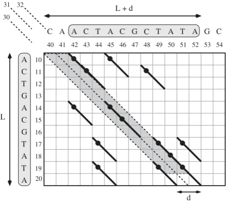
Figure 1 shows an example of an (L, d, 2)-repeat with L = 11 andd= 2.
Searching for multiple repeats means inferring all (L,d, r)-repeats of the input sequence(s), with parametersL,d andrgiven by the user. Since these are computationally hard to find, we propose a preprocessing step to mask out from the input sequences as many positions as possible that cannot belong to a word of lengthLthat is part of an (L,d,r)-repeat. Since this condition is difficult to be quickly verified, we apply filtering conditions that
are based on properties of the q-grams that simulta-neously occur in two words of an (L,d,r)-repeat, as we shall see from now on. Some of the techniques presented here have being used since 1985 by Ukkonen [7] and many other authors, but we follow more closely the definitions, techniques and properties given by Rasmus-sen et al. [6].
Definition 2Given a sequence s, a q-hith is defined as a pair (i,j)such that at positions i and j of s we have the same q-gram, that is s[i,i+q- 1] =w=s[j,j+q- 1].We also say that the word w is the q-gram ofh.For any pair h= (i,j),i(resp.j)isthe first projection (resp. second projection)of h.
Definition 3 Given a q-hit h = (i, j), we say that the diagonal ofh isdiag(h) = {h'= (i',j')|j'-i'=j-i},the set of all possible pairs of positions h' = (i', j') with the same difference of projections j-i.For convenience, we also say that this is the diagonal j - i (note that this number may be negative).We define thedifference of the diagonals ofh= (i,j) and ofh'= (i',j'),in this order,to be the difference(j -i) - (j'-i').We say that two diagonals areconsecutiveif their difference is1or-1.
Figure 1 shows an example of diagonals andq-hits.
Let us consider a wordw=s[a,a+L- 1] of lengthLand another wordw'=s[a',a'+L- 1]. One can notice that if we had an edit distance 0 betweenwandw', then all the L-q+ 1 pairs (a,a'),...,(a+L -q,a'+L-q) would beq -hits (there could be more if the same q-gram occurs at more than one position ofs). Roughly speaking, notice that any edit operation applied to one of the sequences will shift the diagonal of a q-hit by at most 1 and possibly remove at mostq q-hits. Hence, ifwandw'are distant by at mostdedit operations, then there must be at leastp= (L-q+ 1) -qd q-hits. TheTUIUIUfilter verifies this property (first introduced in the proof of Theorem 5.1 of [7]), that is:
there exists for and a set of -hits of size at leaw w′ S q sst p=(L− + −q 1) qd.
(1)
Moreover, in order to make the filtering condition more stringent, we also require that the set above is such that for any pair of q-hitsh= (i,j) andh'= (i',j') in S, the following properties hold:
|diag(h) - diag(h')|≤d (2)
i≠i' (3)
j≠j' (4)
i<i'if and only if j<j' (5) L
d L + d
A C T
G A C
G T A
T A
T A G C
40 41 42 43 44 45 46 47 48 49 50 51 52 53
A C T A C G A
C
54
T A C
10
11
12
13
14
15
16
17
18
19
20 31 32
30
Figure 1
A (L,d, 2)-repeat and a parallelogram. An example a (L,
d, 2)-repeat withL= 11,d= 2. Diagonals 30, 31, and 32 are shown. Among them, 30 and 32 have distance 2, while 30 and 31 (as well as 31 and 32) are consecutive. Assuming thatq= 2, aq-hit is represented by a thicker diagonal of length 2 plus a small black circle representing its pair of coordinates. The
In Figure 1 we can see examples for these properties that we motivate as follows. As mentioned above, an edit operation shifts the diagonal of a q-hit by at most one position. Thus,d edit operations can shift this diagonal by at most d positions, which explains property 2 (already used by the filter in [6]). We now prove that properties 3, 4 and 5 are also necessary conditions. These, to the best of our knowledge, were not used in previous filters while they will be considered inTUIUIU.
Theorem 1if w=s[a,a+L- 1]and w'=s[a',a'+L- 1] are distant by at most d edit operations, then there are at least p= (L-q+ 1) -qd q-hits that pairwise verify properties 3, 4 and 5.
Proof. LetWandW'be sequences on the alphabetΣ∪{-} where '-' ∉Σsuch that:
• there is no i Œ [0, |W| - 1] with both W[i] and W'[i] equal to '-';
• L≤|W| = |W'|≤L +d;
• the sequence obtained fromW (resp.W') by deleting all characters '-' is equal tow(resp.w');
•WandW'are a representation of an optimal alignment betweenwand w'where the symbol '-' represents a gap and with cost function corresponding to the edit distance (0 for a match, 1 for any other edit operation).
Let nowXbe a sequence over the alphabet {M, D} such that:
• |X| = |W| = |W'|;
for allifrom 1 to |X|,X[i] =MifW[i] =W'[i], elseX[i] =D.
We now prove the following lemma.
Lemma 1 There are at least p = (L - q + 1) - qd distinct positions i such that for all jŒ[0,q- 1],X[i+j] =M,that is, at least p= (L-q+ 1) -qd positions i where a run of Ms of size at least q begins.
Proof. Obviously, there can be at most |X| -q+ 1 runs of Ms of size at leastqinX. Furthermore, each characterD inXdestroys at mostqdruns ofMs since there can be at mostd Ds inX. IfNis the number of runs ofMs of size at leastqinX, we thus have:
N≥(|X| -q+ 1) -qd≥(L-q+ 1) -qd
runs ofMs of size at leastqinX. □
By the wayXwas built and from Lemma 1, there are at least (L-q+ 1) -qdruns ofq Ms. Each pair of such runs corresponds to two q-hits themselves corresponding to two distinctq-grams inw(at positionsiandi') and inw' (at positions j and j'), proving conditions 3 and 4. Obviously, if theq-hit (i,j) (resp. (i',j')) occurs first, then i>i'andj>j'(resp.i'>iandj'>j), proving condition 5. □
Observe that the above proof follows a reasoning somewhat similar to the one in [7]. In the remaining of this section, we introduce some terminology that we use to explain the actual steps performed by TUIUIU in order to verify the properties listed above.
For any wordw=s[a,a+L- 1], we want to check whether it belongs to an (L,d,r)-repeat. Suppose this is the case, that is, there exists wordswk, fork= 1, 2,...,r- 1 such that w and wk have edit distance no more than d. For each
pair of words w and wk, the computation of the edit
distance would take as much as θ(dL) time for the best algorithm. Instead, we count the q-hits of these two words and we verify whether they are at leastp, because there must be forwandwka set ofq-hits S that satisfies
property (1). Theq-hits could theoretically be as many as (L - q + 1) × (L + d - q + 1). Nevertheless, if we also consider that property (2) must be satisfied by any pair ofq-hits in S, then we can countq-hits only within the limited region of d + 1 consecutive diagonals (like the diagonals 30, 31 and 32 in Figure 1) which includes no more than (d+ 1) × (L-q+ 1) possibleq-hits. This shows us the convenience of sorting theq-hits by diagonals. Let us formalise this idea by introducing the notion of a parallelogram, that is found in [6].
Definition 4 (parallelogram) Given a word w = s[a,a + L- 1]of length L, and the set of d+ 1consecutive diagonals[c, c+d],with d<L,we define the respective parallelogram as the set of all pairs:
Parall(a,L,c,d) = {(i,j)|iŒ[a,a+L-q],j-iŒ[c,c+d]}.
In Figure 1, the grey highlighted parallelogram represents the parallelogram Parall(10, 11, 30, 2). Notice that the q-hits (19, 49) and (19, 51) (are pairs that)dobelong to Parall(10, 11, 30, 2), according to the definition.
Finally, a pairh= (i,j)ŒParall(a,L,c,d) may or may not be aq-hit, depending on whether or notw[i,i+q- 1] =w [j,j+ q- 1].
Given a wordw=s[a,a+L- 1], the parallelogram Parall (a,L,c,d) is used to check properties (1) and (2) forw against a wordwkthat is candidate to be one of ther- 1
words which, together with w, are part of an (L, d, r )-repeat. This is done in the following way. Letwandwk=s
[u, v] be an (L, d, 2)-repeat, and consider an optimal alignment of these two words. The pairs of matched positions described in this alignment belong to no more thand+ 1 consecutive diagonals. In particular, there is a diagonalcwithcsuch thatuŒ[c+a,c+d+a] andvŒ[c +a+L- 1,c+d+a+L- 1] where the matched positions belong to the union of the diagonalsc,c+ 1,...,c+d. In this case, we say that the parallelogram Parall(a,L,c,d) detectsthis (L,d, 2)-repeat. This is why we can limit the search of the q-hits of w and wk to within the
parallelogram.
Consider now the wordx =s[c+ d+a,c+a+L - 1] of length L - d that is contained in wk, which in turn is
contained in the wordz=s[c+a,c+d+a+L- 1], having lengthL +d. Bothxandzare shown in Figure 2 for the darkest of the two parallelograms.
Notice that, sinced<L,xis well defined becausec+d+a
≤c+a+L- 1. Therefore, we have that any other (L,d, 2)-repeat {w, w′k} detected by the same parallelogram would be such thatwkand w′k overlap because they both contain x. This ensures that, for a wordw, no two non-overlapping repeats could be detected by the same parallelogram.
We say that two parallelograms Parall(a, L, c, d) and Parall(a,L,c',d)overlapif the wordsx=s[c+d+a,c+a+ L- 1] andx'=s[c'+d+a,c'+a+L- 1] overlap. Ifc<c', this happens ifc+a+L- 1≥c'+d+a. In other words, parallelograms Parall(a, L, c, d) and Parall(a, L, c', d) overlap if and only if
|c'-c| <L-d.
In Figure 2 we can see two parallelograms that overlap, where the overlapp=s[c'+d+a,c+a+L- 1] betweenx andx'is highlighted.
In general, if Parall(a,L,c,d) detects the (L,d, 2)-repeat w=s[a,a+L- 1] andwk=s[u,v], and Parall(a,L,c',d)
detects the (L,d, 2)-repeatw=s[a,a+L- 1] and w′k =s [u',v'], and if the two parallelograms overlap, then the wordswk=s[u,v] and w′k =s[u',v'] also overlap. We say that a set of parallelograms isnon-overlappingif no two of them overlap.
Sincew=s[a,a+L- 1] andwk=s[u,u+L'- 1] are two
words with edit distance no more thand, the existence of a set of q-hits S that satisfies properties (1) and (2) implies that there are at least p q-hits inside a parallelogram Parall(a, L, c,d) with c such thata + c≤ u ≤a+c+d.
We say that a parallelogram isfineif there are at leastp q -hits inside the parallelogram. For example, the paralle-logram highlighted in Figure 1 is fine, with a set S′ of 8 q-hits inside. This leads us to our first filtering condition, that is easy to be efficiently checked:
for any word w=s[a,a+L- 1],we keep the positions in the interval[a,a+L- 1]if there exist at least rfine non-overlapping parallelogramsParall(a, L,ci, d), with ci Œ
{c1,...,cr}.
It is worth noticing that w itself generates a fine parallelogram, which explains why we check the
L w
a+L−1 a
d d
z p
c’+a+L−1
c’+d+a+L−1
c+a
x
x’
c+a+L−1
c+d+a+L−1
c+d+a
c’+a c’+d+a
c c’
Figure 2
Detection of (L,d,r)-repeats and two overlapping parallelograms. Two parallelograms that overlap. The dark grey parallelogram in the figure detectsq-hits betweenw=s
[a,a+L- 1] and any wordwk=s[i,j] withiŒ[c+a,c+d+
a] andjŒ[c+a+L- 1,c+d+a+L- 1]. The wordz=s[c+
a,c +d+ a+ L- 1] of lengthL+dcontains the wordwk
which in turn contains the wordx=s[c+d+a,c+a+L- 1] of lengthL-d. Analogously for the light gray parallelogram, the wordz'= s[c'+ a,c'+ d+a+L- 1] of lengthL+ d
contains a word w′k which in turn contains the wordx'= s
[c'+d+a,c'+a+L- 1] of lengthL-d. The wordswkand
′
wk are not shown because their length is variable. They
necessarily overlap because they both contain the wordp=s
existence of r fine non-overlapping parallelograms instead ofr- 1.
We are now going to see two more stringent filtering conditions leading to the additional conditions actually applied byTUIUIU.
First, we require that the set of q-hits inside the parallelogram satisfy property (3). This property simply ensures that two distinctq-hits of S do not share a first projection. We say that a parallelogram is good if and only if there are at leastp q-hits inside the parallelogram such that no two of these q-hits have the same first projection. In Figure 1, the set S contains 7q-hits that pairwise satisfy property (3), and hence the highlighted parallelogram is good. This leads us to our second filtering condition that is also easy to be efficiently checked:
for any word w=s[a,a+L- 1],we keep the positions in the interval[a,a+L- 1]if there exist at least rgood non-overlapping parallelograms Parall(a, L,ci, d), with ci Œ
{c1,...,cr}.
Second, we can further require that the set of q-hits S inside Parall(a,L,c,d) satisfies also property (5). We say that a good parallelogram isexcellentif and only if there are at leastp q-hits inside the parallelogram such that any two of them satisfy property (5). Given that S contains distinctq-hits, we have that, if property (5) holds for all pairs ofq-hits in S, then properties (3) and (4) also do. Therefore, requiring property (5) for S guarantees that properties (3) and (4) hold as well. In Figure 1, the set S of 7 q-hits satisfies property (5) and, indeed, also satisfies property (3) and property (4). In fact, the highlighted parallelogram is excellent. This leads us to our third and last filtering condition that can be expected to be efficiently checked for general cases:
for any word w=s[a,a+L- 1],we keep the positions in the interval[a,a+L- 1]if there exist at least rexcellent non-overlapping parallelogramsParall(a,L,ci,d),with ci Œ{c1,...,cr}.
Necessary condition applied byTUIUIU
Given a sequence sand the parametersL,d,rdescribed above,TUIUIUtries to keep only those positions ofsinside an interval [a,a+L- 1] such that the wordw=s[a,a+L -1] of length L belongs to an (L,d,r)-repeat. Since this condition is hard to be efficiently verified, only necessary conditions are checked:
for any interval[a,a+L- 1],TUIUIUkeeps these positions if there exists at least rexcellent (orfineor goodif the
user so prefers)non-overlapping parallelograms Parall(a, L,ci,d),with ciŒ{c1,...,cr}.
Description of the algorithm
We now give an overview of the algorithm applied by TUIUIUwhose pseudocode is provided in Appendix 1.
For any possible q-gram, we build the list of all its occurrences ins. The sum of the sizes of the |Σ|qoccurrences lists isn-q+ 1. They are concatenated and stored in an array ofn-q+ 1 positions and are accessed through |Σ|qpointers, one for each possibleq-gram (line 1).
We move a sliding windoww=s[i,i+L- 1] of lengthL alongsand onlyq-hits relative to this sliding window are considered. For each positioni, we have to consider all possible parallelograms, i.e. Parall(i,L,c,d) forcŒ[-i,n -i-d+ 1].
Thus, in order to quickly verify which parallelograms are fine, we associate aq-hit counter to every parallelogram. First, counters are initialised for the position zero of the sliding window (lines 1 and 1). This initialisation is straightforward: for allq-grams occurring in [0,L-q], we check whether they create at least one q-hit in each parallelogram. If this is the case, the corresponding parallelogram counters are increased by one. Once the window is slided from positioni- 1 to positioni, theq -hits involving theq-gram that occurs at positioni- 1 are not considered anymore, while those involving the "new" q-gram at positioni+L-qhave to be taken into account. In terms of parallelograms, this corresponds to observing that the parallelograms Parall(i- 1,L,c,d) and Parall(i,L, c,d) differ only by the pairs (i- 1,j) and (i+L-q,j) forjŒ [c,c+d]. Therefore, in order to obtain the number ofq -hits in Parall(i,L,c,d), we only need to subtract from the number ofq-hits in Parall(i- 1,L,c,d), the number ofq -hits of the form (i- 1,j) forjŒ[c,c+d], and we have to add the number ofq-hits of the form (i+L-q,j) for jŒ[c,c+ d]. Thus, when sliding the window insfrom positioni- 1 toi, we just have to consider all occurrences of theq-grams s[i- 1,i+q- 2] (that are leaving) and those ofs[i+L-q,i+ L- 1] (that are entering) and do the following (lines 1 and 1 of algorithm 1). For any occurrencejof the enteringq -gram, we have aq-hit (i+L-q,j) and we increment the counters (line 1) of all parallelograms to which thisq-hit belongs to. Conversely, for any occurrencejof the leaving q-gram, we have aq-hit (i- 1,j) that no longer involves the word of the current sliding window, and hence we decrement the counters (line 1) of all the parallelograms it belongs.
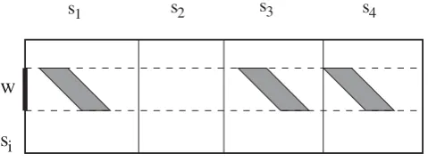
belongs to the parallelograms Parall(i,L, (i-j) -k,d) for kŒ[0,d]. As a result, for eachq-hit, we should updated + 1 counters. In order to reduce this number, we apply a strategy that was already used both in SWIFT[6] and in
QUASAR[4]. We enlarge the parallelogram from d + 1
diagonals tod+bdiagonals (SWIFTactually usesd+b+ 1 diagonals.) whereb≥1. Recall that to avoid the possible presence of two non overlapping occurrences of a repeat in the same parallelogram, we must have that the width of the parallelogram should not exceed L, and henceb must be such thatd +b<L.
In this way, the parallelograms Parall(i,L,k,d) forkŒ[c, c+b- 1] are joined in theenlargedparallelogram Parall(i, L,c,d +b- 1). In practice, this means setting a unique counter for all Parall(i, L, k,d) with kŒ [c,c + b - 1]. Therefore, in order to search for repeats in the whole input sequence, instead of considering all Parall(i,L,c,d) forcŒ[-i,n-i-d+ 1], it is enough to check for Parall(i, L,c,d+b- 1) withc=k'b, for k′ ∈ − ⎢⎣ ⎥⎦ ⎡⎢⎢[ bi , n i− − +b(d 1)⎥⎥⎤], because every parallelogram Parall(i,L,c,d) is contained in one of these enlarged parallelograms (see Figure 3 for an example). The reason for this modification is that
now aq-hit can only be shared by ⎡⎢⎢d bb+ ⎤⎥⎥ parallelograms.
Thus, from d+ 1 updates perq-hit, we reduce to d b b
+ ⎡ ⎢⎢ ⎤⎥⎥ updates per q-hit. This means 2 updates perq-hit if as default value. For b we adopt the smallest power of 2 (speeding up the divisions by b) greater than d, like in [6]. Since b parallelograms will be combined into one enlarged parallelogram, the probability that one enlarged parallelogram is judged to be fine/good/ excellent increases. As concerns the filtering conditions,
we just replace parallelograms that deal with d + 1 diagonals with parallelograms that deal with d + b diagonals. The filter remains lossless, but this enlarge-ment of the parallelograms implies that it may not be as selective as it could be. On the other hand, this enlargement makes the filter much faster.
Back to the pseudocode shown in Algorithm 1, for each value of j, line 1 now updates up to d b
b
+ ⎡
⎢⎢ ⎤⎥⎥ counters. When a counter reaches p, then the corresponding parallelogram is fine. Since we can also easily check what was the last updated counter, and since the occurrences lists are ordered, we can also only update counters that were not yet updated by the current occurrences list (line 1). This allows us to easily count first projections of q-hits instead of simply counting q -hits. Doing this, when the counter of q-hit projections reachesp, then we directly detect that the corresponding parallelogram is good (line 1).
For a given sliding windoww=s[i,i+L - 1], we search for excellent parallelograms (line 1) only if at least r good parallelograms are detected (line 1). If at least r excellent parallelograms are detected among the good parallelograms, all the positions [i,i+L- 1] correspond-ing to this slidcorrespond-ing window ware kept by the filter (line 1). We are now going to see how we check whether a good parallelogram is excellent.
Consider two wordswandw'and also a set S ofq-hits, relative to these words, that satisfy property (5). In order to check this property, one has to detect if at least p q -grams occur in the same order in w and w'. To this purpose, we consider the length of the longest common ordered subset ofq-grams occurring both inwandw'.
In practice, we define a new alphabet Σq in such a way that every possible q-gram (any sequence of qletters in
Σ) corresponds to a symbol a in Σq, thus |Σq| = |Σ|q. Given a sequencesonΣ, we transform it into a sequence
s on Σq replacing from left to right the letters[i]ŒΣby the symbol in Σq corresponding to theq-gram starting at
position i of s. Note that |s| = |s| - q + 1. On the Σq alphabet, the longest common ordered subset ofq-grams occurring both inwandw'is a common subsequence of
w and w′. In particular, if we were interested in looking for the largest set S ofq-hits that satisfies property (5), it would be enough to compute the LCS of w and w′, which is a very well studied problem. Given that our third filtering condition, where we must test whether a
w L
b d
d b
Figure 3
Enlarging parallelograms fromd+ 1 tod+b
parallelogram is excellent or not, also requires that allq -hits of S belong to a parallelogram, then we define the following problem:
Definition 5 (Parallelogramq-hits Chaining Problem) Given a word w=s[a+L- 1]and a parallelogramParall(a, L, c, d), we want to exhibit a set Sof q-hits inside this parallelogram with largest size that satisfies property (5).
Hence, in order to check at line 1 of Algorithm 1 if a good parallelogram is excellent, we solve the Parallelo-gramq-hits Chaining Problem for this parallelogram and check if the size of the obtained set S is at least p. In order to solve the Parallelogram q-hits Chaining Pro-blem, many strategies could be used, ranging from a simple dynamic programming approach within the parallelogram (strategy PDP for Parallelogram Dynamic Programming) to a sparse dynamic programming approach that takes advantage from the fact that few q -hits are expected on average. For the sparse solution, we used a reimplementation of Hunt and Szymanski's [17] algorithm that was presented by Gusfield in [18] using the computation of a LIS (Longest Increasing Subse-quence). In this reimplementation, for each a Œ Σq from the first word, we should provide the occurrence list of a in the second word. In our modified algorithm, only occurrences relative to q-hits inside the parallelo-gram are considered. In order to provide this set of truncated occurrences lists, we perform L -q+ 1 binary searches in the occurrences lists. We call this thestrategy PHS (for Parallelogram Hunt Szymanski). As an alter-native, a chaining [18] algorithm applied to the set ofq -hits inside the parallelogram could also be used, but no theoretical improvement could be expected against strategy PHS.
Moreover, we have designed an optimisation that uses some simple incremental information from the test for the sliding windoww=s[i,i+L- 1] in order to possibly avoid such test for the next sliding windows. This works as follows. Consider a parallelogram P for the sliding windoww=s[a- 1,a+L - 2] for which the solution of the Parallelogramq-hits Chaining Problem resulted in a set ofℓq-hits. After sliding the window fromwtow'=s [a,a +L - 1], and sliding P consequently, solving the Parallelogramq-hits Chaining Problem results in eitherℓ - 1, or ℓ, or ℓ + 1 chaining q-hits. Hence, only parallelograms P whose value forℓwas equal to either p- 1,porp+ 1 for positiona- 1 (wordw) have a chance to become or stay excellent parallelograms for positiona (word w') as well. This motivates the following optimisation: we address the Parallelogram q-hits Chaining Problem only for parallelograms whose pre-vious solution for it wasp- 1,porp+ 1. Done on top of
strategyPHS, this is what we callstrategy PQCPbecause it is our actual solution for the Parallelogram q-hits Chaining Problem as we motivate later with experi-mental results.
In order to check for non-overlapping repeats only, given a set of good/excellent parallelograms, both at lines 1 and 1, we look for a subset of non-overlapping parallelograms with maximal cardinality. This can easily be done by applying the following greedy strategy to the sequence of parallelograms ordered by increasing start-ing diagonals. Let Parall(a,L,c,d+b- 1) and Parall(a,L, c',d +b- 1) be two consecutive parallelograms, in this order, each one withd+bdiagonals, and let Parall(a,L, c", d + b - 1) be the next one. If the first two parallelograms overlap (which means that c' -c<L - (d + b- 1)), then we can remove the second one from the sequence and repeat the process for the two consecutive parallelograms Parall(a,L,c,d+b- 1) and Parall(a,L,c", d + b - 1) in the remaining sequence. If they do not overlap, then we can keep the first one in the set and repeat the process with the next two consecutive parallelograms in the sequence: Parall(a, L, c', d + b -1) and Parall(a,L,c",d+b- 1). This procedure runs in linear time. As mentioned in the introduction, and as the names suggest, the version ofTUIUIUthat checks for fine parallelograms is named FINE, while the version that checks for good (resp. excellent) parallelograms is namedGOOD (resp.EXCELLENT).
Looking for repeats across multiple sequences withTUIUIU* In this section, we describe what is done in order to look for repeats across multiple sequences, modifying TUIUIU into TUIUIU*. Consider an integer m ≥ 2 and a set of sequencess1,s2,...,sm. In the set of sequencess1, s2,...,sm,
an (L,d,r)-repeat is defined as a set ofr≤mwords such that given any pair of them, their edit distance is at most dand they occur in distinct sequences (recall that, in this context, we use the term word for a contiguous segment of one of the sequencess1,s2,...,sm).
Simple modifications of the algorithms FINE, GOOD and
EXCELLENT are done in order to deal with these new
requirements, generating the corresponding algorithms FINE*,GOOD* andEXCELLENT* that are then applied to the concatenationsofs1,s2,...,sm. While sliding the window
on the wordwalong a sequence, saysi, we look for fine/
good/excellent parallelograms in all other sequences as shown in Figure 4. If fine/good/excellent parallelograms are detected in at least r - 1 other sequences (different fromsi), then we keep the wordw. Indeed, when testing
a wordwfrom a sequencesi, we test parallelograms from
sequence sj for j ≠ i, in order to avoid to compare si
but as soon as a desired excellent parallelogram is detected in a sequencesj, we skip the remaining ofsjand
go to the next sequence. Finally, if already r excellent parallelograms are detected, we keepwand try the next position. No overlap checking is done, since all obtained parallelograms detect repeated words, other thanw, from different sequences.
Complexity analysis
In theTUIUIU* framework, we considernas the sum of the sequences length, while in theTUIUIUframeworknis the length of this sequence. Hence, the input size is in both cases n. In this way, the complexity analysis is actually the same forTUIUIUandTUIUIU*.
We present a complexity analysis for EXCELLENT (which holds forEXCELLENT* too), whose pseudocode is presented in Algorithm 1. At the end, we also consider the complexity analysis ofFINE (which holds also forFINE*), and ofGOOD(that is the same asGOOD*). Observe that no complexity comparison is done with any other q-gram based filtering tool asTUIUIUis the first tool for filtering multiple repeats with edit distance.
In order to have better parameters for the complexity analysis, besides the lengthnof sequences, we consider also h to be the number of q-hits andc the number of non-avoided computations of the Parallelogram q-hits Chaining Problem at line 1. For an average analysis, we consider the average number based on a random uniform distribution ofncharacters fromΣ.
Concerning space usage, as described in Section "Description of the algorithm", the main data structure, theq-gram index built in line 1, uses an array withn-q+ 1 integers and another with |Σ|q pointers/integers. Its construction is done by applying a simple counting sort on the sequence of q-grams s. This takes time O(n +
|Σ|q), that isO(n) if we can suppose thatq≤log|Σ|n. All other data structures also requireO(n) memory: we have
n b
⎢
⎣⎢ ⎥⎦⎥ counters for all current parallelograms and ⎢⎣⎢nb⎥⎦⎥ skip positions (in order to avoid computations of the Parallelogramq-hits Chaining Problem, as we described the difference between strategies PQCP and PHS).
Concerning time, a critical parameter is the numberhof q-hits. With the loops at lines 1 and 1, for eachq-hit, we
update up to ⎡⎢⎢d bb+ ⎤⎥⎥ counters at lines 1 and 1. At line 1,
we execute all theccomputations of the Parallelogramq -hits Chaining Problem. Using the strategy PQCP (or PHS), each Parallelogram q-hits Chaining Problem is solved inO(Llogk+ylogL), wherekis the size of theq -gram occurrence list andyis the number ofq-hits inside the parallelogram. Therefore, each Parallelogram q-hits Chaining Problem is solved inO(Llogn+L(b+d) logL)
time in the worst case and O L( log Σnq +Llog )L on average, assuming that the q-hits are sparse (as we observed in practical tests). As a result, time complexity
is O(d b+b h+cL(logn+(b+d) log )L in the worst case,
and O d bb h cL nL
q
( + + log )
Σ on average.
Let us now estimate the values forh andc. In the worst case (s = an), h = n2, but on average, h = n2|Σ|-q. As concerns c, there are at most n
b
⎢
⎣⎢ ⎥⎦⎥ good parallelograms for each position of the sliding window, thus in the
worst case we havec=n n b
⎢
⎣⎢ ⎥⎦⎥. As a first approximation, we are assuming a slightly stronger hypothesis about the sequence, a random uniform q-gram distribution. We can expect the probability that a parallelogram is fine
(good) to be x
i
q i i p
L q⎛
⎝ ⎜ ⎞
⎠
⎟ −
=
−
( )
∑
Σ , wherex= (L-q+ 1)(d+ b) is the size of a parallelogram andp= (L-q+ 1) -qd. Using Stirling's formula and the fact that for typical valuesx|Σ|-qe<p, we havex
i O xe p q
i p L q
iq p
⎛ ⎝
⎜ ⎞
⎠
⎟ =
= −
−
∑
ΣΣ
(( ) ).
Therefore, the expected number of fine (good) paralle-lograms is
n b
xe p q
p
2
Σ ⎛
⎝ ⎜ ⎜
⎞
⎠ ⎟ ⎟
s1 s2
s
is3 s4
w
Figure 4
Application to multiple sequences. Application of
TUIUIU* to multiple sequences. For a sliding windowwon a
sequencesi, parallelograms are tested on all other sequences.
and c n b xe p q p = ⎛ ⎝ ⎜ ⎜⎜ ⎞ ⎠ ⎟ ⎟⎟ 2
Σ , for anyr. The worst case time complexity is then
O b d b n
n
b L n b d L O
n
b L n b d L
+ + + + ⎛ ⎝ ⎜ ⎜ ⎞ ⎠ ⎟ ⎟= + + ⎛ ⎝ ⎜ ⎜
2 2 (log ( ) log 2 (log ( ) )⎞⎞
⎠ ⎟ ⎟,
and the average complexity is
O b d b n
n b
L q d b e p q p L nL q q + + ⎛ − + + ⎝ ⎜ ⎜ ⎞ ⎠ ⎟ ⎟ ⎛ ⎝ ⎜ ⎜ ⎜ ⎞ ⎠ ⎟ ⎟ ⎟ −
2 Σ 2 1
Σ Σ
( )( )
log .
Notice that the second part in the sum decreases as p increases. Forplarge enough, the average time complex-ity is
O b d b n q + ⎛ ⎝⎜ ⎞ ⎠⎟ −
2 Σ .
Finally, the complexity ofFINEandGOODare obtained by simply settingc= 0.
Results and discussion
We now report a battery of experimental tests that were applied toTUIUIUwith different filtering conditions (FINE,
GOOD and EXCELLENT) and strategies for solving the
Parallelogramq-hits Chaining Problem. As input, TUIUIU receives a sequencesand a set of parametersL,d,r, and q. For parameterb,TUIUIUtakes as default value the same as adopted in [6]: the smallest power of 2 greater thand. Moreover, we give the user flexibility for the choice of which filtering condition to apply. As output, the user obtains a sequence where every position that does not satisfy the conditions is masked by TUIUIU. Since we do not know any other work that is a filter for multiple repeats, in particular with the same kind of output, we do not compareTUIUIUdirectly to other methods, but try instead to reproduce as much as possible the filtering conditions used by such approaches. In this sense, the closest method we compare TUIUIU to is SWIFT. Even though we did not report it here, we also found that the strategy of countingq-hits inside parallelograms used in SWIFTperforms better than the strategy of countingq-hits inside rectangles (as is done in QUASAR[4], for instance), as it was already reported in [6]. Roughly speaking,SWIFT is a BLAST-like tool where the seeds for similarity expansions are provided not by exact matches of length W asBLASTdoes, but by an (L,d, 2)-repeat found by using a filter that is at the core of the SWIFT algorithm. Improving on speed seems to have been an important issue in the development of SWIFT, which also implies that we did not see reported in the paper error levels above 5%. TUIUIU can deal with bigger error levels, for
instance up to 14% of the size of the repeat sought. This implies that a smaller value should be used for parameter q, and hence, that longer running times are unavoidable.
We start by giving a few definitions of the values that we used to evaluate the results obtained. The quality of the filtered output is measured by the ratio between the total length of the non-filtered sequence and its original length. We call this the selectiveness of the filter. The smaller the selectiveness, the better. On the other hand, the main resource consumed by the algoritm is the running timethatTUIUIUtakes. If we compare methods A and B, in this order, the selectiveness improvement (SI) is the quotient between the selectiveness of B and the selectiveness of A. Accordingly, we define the speedup factor(SU) of the algorithm to be the quotient between the running time spent by A and the running time spent by B. We also define the slowdown factor (SD) to be the inverse of the speedup factor. For convenience, we quite often refer to a SI/SU/SD ofx% if the SI/SU/SD factor is 1 + x/100. For instance, a speedup factor 1.02 may be reported as a speedup of 2%. The experiments were run on an AMD Athlon(tm) 64 Processor 3500+ machine with 4 Gigabytes and running Linux for amd64.
Time and selectiveness on randomly generated sequences
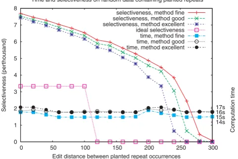
We first present some tests performed on short randomly generated sequences. Each dataset is composed of five sequences of length 300 kb each, generated using a Bernoulli model (each nucleotide occurring with fre-quency 14). Every sequence contains exactly one occurrence of a repetition of length 1 kb, the occurrences being distant from each other by at most X edit operations, with Xranging from 0 to 300 (that is, from 0 to 30% of the repeats length). The datasets were filtered using the methodsFINE,GOODandEXCELLENT, with parametersL= 1000,d= 100,r= 5 andq= 6 (looking for repetitions of length 1000 allowing for up to 10% differences). The results are shown in Figure 5. One can see that the computation time is only slightly influenced by the nature of the repeat, and that in this case approximately 16 seconds are required for filtering the 1.5 Mb dataset. The ideal selectiveness (in the case of absence of false positives), would be 0.33% forXfrom 0 to 100, and 0 for bigger values of X. As expected, one observes that the selectiveness results are better for EXCELLENTthan forGOOD, which themselves are better than forFINE.
Extensive tests with Neisseria meningitidis strain MC58
Chaining Problem), we used a wide collection of parameter sets, applied to the DNA sequence of the Neisseria meningitidisstrain MC58.Neisseriagenomes are known for the abundance and diversity of their repetitive DNA in terms of size and structure [19]. The size of the repeated elements range from 10 bases to more than 2000 bases, and their number, depending on the type of the repeated element, may reach more than 200 copies. This fact explains why theN. meningitidis MC58genomic sequence, with 2.3 Mb, has already been used as a test case for programs identifying repeats like in [12].
The best strategy for solving the Parallelogram q-hits Chaining Problem
In order to solve the Parallelogram q-hits Chaining Problem, we tested the three possible strategies described in the "Description of Algorithm 1" section. For any instance of this problem, the PDP strategy has running time proportional to the size of the parallelogram, which is (L - q + 1) × (d + b). On the other hand, the PHS strategy is expected to take time proportional to
( logL nq ylog )L
Σ + , where y is the number of q-hits inside the parallelogram. Notice that y has a strong dependence on q. Increasing q, we decrease the prob-ability of a q-hit and consequently we decrease y. We may expect thaty=O(L) on average, for not too smallq. Indeed, multiplying the expected probabilityΣ-q of aq -hit by the size (L -q + 1)(d +b) of a parallelogram, we may expect thaty=O(Σ-qdL) on average, or simplyy=O
(L) for not too small values of q. Therefore, we expect PHS to be faster than PDP.
As concerns the PQCP strategy, it is very difficult to predict how many computations of the Parallelogramq -hits Chaining Problem are avoided with the optimisa-tion it realises. The same complexity as PHS certainly holds, but we definitely expect it to be faster. The reason is that EXCELLENT parallelograms tend to be clustered together, or in other terms, parallelograms that fulfill the conditions (2), (3), (4) and (5) are usually not isolated. This happens because the probability of two adjacent parallelograms to be EXCELLENT is not independent: parallelograms close to an EXCELLENT one have an increased probability to be EXCELLENT too. To sum up, from a theoretical point of view, PQCP should be faster than PHS, which in turn should be faster than PDP.
In practice, these expectations were confirmed in the 72 tests we made with different sets of parameters on MC58. In all cases except one, the running time for the PHS strategy did not get worse in comparison to the simple PDP. In fact, the overall observed running time improvement from PDP to PHS was 1.57. In all tests, PQCP performed faster than PHS and the overall observed running time improvement from PHS to PQCP was 1.88. Hence, in all tests PQCP performed faster than the simple PDP and the overall observed running time improvement from PDP to PQCP was 3.22. Since all three strategies provide the same selectiveness, but for some cases PDP was 18 times slower than PQCP, we discarded strategies PDP and PHS from the subsequent systematic comparisons when we have to solve the Parallelogram q-hits Chaining Problem.
TheFINE,GOOD,EXCELLENTvariants ofTUIUIU
In the Section "Methods", we saw three possible filtering conditions, depending on what kind of non-overlapping parallelograms we would like to find: fine, good, or excellent. All three filters ensure that all (L,d,r)-repeats are kept, so they are all lossless. In Section "Description of the algorithm", we saw the description of Algorithm 1, that implements a filter (EXCELLENT) for the third filter condition. If we remove lines from 1 to 1, we have a filter (GOOD) for the second filter condition. Moreover, if we also update all parallelogram counters (line 1) instead of only new ones as described in Section "Description of the algorithm", we have a filter (FINE) for the first filter condition. It should be said that SWIFT[6] identifies a parallelogram as a similarity region (for r = 2) if the parallelogram is FINE. In other words, the comparison to FINE is in some sense a comparison to the conditions applied bySWIFTfor finding (L,d,r)-repeats forr= 2.
0 1 2 3 4 5 6 7 8
0 50 100 150 200 250 300
17s 16s 15s 14s
Selectiveness (perthousand)
Computation time
Edit distance between planted repeat occurrences Time and selectiveness on random data containing planted repeats
selectiveness, method fine selectiveness, method good selectiveness, method excellent ideal selectiveness time, method fine time, method good time, method excellent
Figure 5
Tests on random generated sequences. Application of the three versions ofTUIUIUwith parameters (L,d,r) = (1000,
As concerns the parameter sets we used for the three algorithms when applied to MC58, we selected all combinations such that:
L d L r q
= = = =
50 100 200 4 10 12 14 5 8 13
14 13 12 11 10 , , ;
/ %, %, %, %;
, , ;
, , , , , 99 8 7 6 5 4, , , , , ;
and such that the restriction
p= (L-q+ 1) -qd≥TL,
for τ = 0.08, was satisfied. This restriction was adopted because if the thresholdpis too small, the selectiveness for any method gets bad–as one should expect–as does the running time, in particular forEXCELLENT. For instance, for L, d, r, q = 100, 14, 5, 6 (p = 11) we obtain a selectiveness of 99.992%, 99.957% and 99.835% for the methods FINE, GOOD and EXCELLENT, respectively. In this case, EXCELLENT is 9.36 times slower thanGOOD. For this reason, in order not to spend too much running time on testing cases that would never be used anyway since the
selectiveness is bad, we empirically chose a threshold factorτ= 0.08 forp/L. This resulted in 198 combinations forqranging from 4 to 14. The combinations are split in 99 low error cases (d/L= 4%) and 99 large error cases (d/ L= 10%, 12%, 14%). We are now going to comment the results reported in Table 1.
VariantsGOODversusFINE
We start with the comparison between FINE and GOOD. The methods are quite similar, except for an extra verification depending on whether the counter of a parallelogram to which a q-hit belongs was already updated or not for the current occurrences list. This extra checking introduces a small slowdown: an almost uniform slowdown of 3.2% is indeed observed in 195 out of 198 cases. In the three cases whereL= 200,d= 28, r= 5, 8, 13,q= 4–the 3 cases where the ratio betweenp and the expected number ofq-hits in the parallelogram is smaller (85/46.2 = 1.8) – FINE was 78% slower than GOOD. These 3 degenerated cases are discarded from the subsequent running time analysis, but not discarded from the analysis of selectiveness. On the other hand, the selectiveness for GOOD is always better. Overall, in
Table 1:FINE/GOOD/EXCELLENTsystematic comparison on MC58 sequence
RESTRICTION NB.TESTS EXCEL.SEL. GOOD/FINE EXCEL./GOOD EXCEL./FINE
SI SD SI SD SI SD
overall 198 11.19 1.685 1.032 1.307 1.752 2.309 1.811
d/L≥10% 99 18.45 2.302 1.043 1.508 2.062 3.428 2.166
d/L= 4% 99 3.93 1.067 1.021 1.107 1.441 1.191 1.467
q< 7 105 14.41 2.274 1.043 1.506 1.533 3.377 1.236
q≥7 93 7.56 1.019 1.019 1.082 1.998 1.104 2.039
p/L≥25% 159 5.90 1.820 1.033 1.347 1.321 2.546 1.236
p/L< 25% 39 32.77 1.135 1.027 1.146 3.506 1.347 3.614
p/L> 14% 183 8.99 1.720 1.031 1.312 1.415 2.363 1.457
p/L≤14% 15 38.07 1.246 1.038 1.244 5.854 1.653 6.067
L= 200 69 6.42 1.958 1.044 1.456 1.744 2.829 1.835
L= 100 69 12.35 1.611 1.032 1.172 2.018 2.113 2.077
L= 50 60 15.35 1.454 1.019 1.292 1.454 1.938 1.479
r= 13 66 8.44 1.745 1.033 1.323 1.729 2.45 1.791
r= 8 66 11.11 1.677 1.032 1.302 1.756 2.280 1.817
r= 5 66 14.03 1.632 1.030 1.297 1.770 2.196 1.825
d/L≥10%,p/L≥25% 66 8.79 2.874 1.049 1.689 1.205 4.451 1.236
q< 7,d/L≥10% 78 18.42 2.631 1.047 1.626 1.710 4.038 1.800
q< 7,d/L≥25% 90 6.99 2.446 1.045 1.554 1.138 3.670 1.181
d/L≥10%,p/L≥25%,q< 7 63 8.78 2.962 1.050 1.722 1.188 4.614 1.237
contrast to a running time slowdown of 3.2%, we observe 68.5% of selectiveness improvement on average. In Table 1, we see comparisons of GOOD against FINE restricted to the cases where certain constraints are satisfied. In this way, we can see the influence of several parameters on how much improvement we can expect fromGOOD. Only in cases whereqis bigger (q>= 7), no clear advantage from FINE to GOOD is observed; in fact, little difference can be observed in these cases, since the ratios are very close to 1. The advantage ofGOODoverFINE is clearer for the following cases: large error rates (d/L≥ 10%), smaller q(q< 7), larger p, longer L, and largerr. Combinations of these restrictions improve even more the selectiveness. We have thus verified that looking for good parallelograms (as inGOODand asTUIUIUallows the user to do) is clearly better than looking for FINE parallelograms (as FINE and SWIFTdo) for smaller values ofq, that are also required if we want to deal with larger error rates as we have done here.
VariantsEXCELLENTversusGOOD
We now compareGOODandEXCELLENT. If on one hand, the algorithmic differences between FINEandGOOD are quite small, the differences between GOOD and EXCELLENT are more complex mainly due to the solutions of the Parallelogram q-hits Chaining Problem required at line 1 of Algorithm 1. When property (5) was conceived in the design of TUIUIU, we understood that this could be a good strategy for larger rather than for smaller errors. If the parallelogram is "narrow", it is more likely that any pair of q-hits does already satisfy property (5). We further supposed that the extra cost of solving the Parallelogramq-hits Chaining Problem would be smaller for higher values of thresholdp. What Table 1 shows us is in agreement with these expectations, since for the cases in which d/L ≥ 10% and p/L ≥ 25%, we obtain a selectiveness improvement of 69% in contrast to a time slowdown of 20%. Moreover, we could verify that the cases where the time slowdown is higher are those where p/Lis lower. For instance, we observed that the 15 cases with time slowdown higher than 4 (ranging from 4.28 to 9.36, with average 5.85) are exactly the 15 cases wherep/ L ≤ 14%, and we can still verify a selectiveness improvement of 55% in contrast to a time slowdown of 38% for large error cases (d/L≥10%) withp/L> 14% (not shown on Table 1).
On one hand, EXCELLENT always has better selectiveness thanGOOD(at least equal). On the other hand, the time slowdown may not be worth it. In particular, deciding whether the time slowdown is worthwhile or not depends very much on the application the filtered sequence will be submitted to. For instance, if we have a selectiveness improvement of 30% against a slowdown
of 75% (like the general average numbers for all 198 cases), it may still be worth it if the algorithm we are going to submit the filtered sequence to is, for instance, cubic, since 1.33> 1.75. Anyway, any slowdown above 4 means that we should also consider decreasing q by 1, instead of changing the algorithm from GOOD to EXCELLENT, since this is the expected slowdown for this decrease. Unfortunatelly, this does not guarantee that selectiveness will improve. Moreover, inspecting the cases where q ≥ 7 and p/L ≥ 25%, one may expect the slowdown to increase ifqalso increases.
VariantsEXCELLENTversusFINE
In order to complete these comparisons based on MC58, we proceed with the comparison between FINE and EXCELLENT. Here, like in the previous comparison, but now with even more striking numbers, it is clear that EXCELLENT performs better thanFINE, bringing a selective-ness improvement of 4.45 against a time slowdown of only 25% for error cases larger thanp/L≥25%. Overall, except for three degenerated cases where EXCELLENT got 23% faster thanFINE, we obtained an average slowdown of 81% with a selectiveness improvement of 130%.
Extra tests on Human Chromosome 22
Unfortunately, thresholds such as those present in expressions like p/L >= 0.08, 14%, 25%, q < 7, d/L ≥ 10, depend very much on the parameters L,r,dand on the sequence s that is processed. If the sequence s is known to have abundant repeats, it is expected that TUIUIU will not be able to provide selectiveness better than what is imposed by the repeats present in the sequence. For instance, the human genome has a high level of ALU repeats. There is an unpublished report of a fragment of ALU Y of length 266 that repeats more than 280 times on the human cromossome 22. We decided to apply TUIUIUon this data (last assembly from University Santa Cruz, California, total length 50 Mbases, 15 Mbases of which are unknown and replaced by "N"), with parameters:L,d,r= 260, 13, 280 andq= 14, 13, 12, 11, 10, 9. Results are reported in Table 2. We observe that in all these casesGOODis faster thanFINE(24% faster on average), as in what we called degenerated cases in the MC58 analysis.
Selectiveness was even better, with an average improve-ment of 38.3%. In these cases, we can also observe that the selectiveness improvement fromEXCELLENToverGOOD, even if small, seems to compensate for the slowdown whenq< 12, as Table 2 shows.
increasing q may not lead to a faster execution of EXCELLENT, since the fastest execution was obtained forq= 12. This U-type curve is illustrated by Figure 6.
In order to show the behaviour ofTUIUIUwhen parameter ris changed, we refer to Figure 7, whererchanges in a log scale from 9 to 3200. Notice that the running time of EXCELLENT decreases and selectiveness of all variants increases, as r increases. The running times of GOOD and FINE do not change. As we saw in Figure 6 and in Table 2, this parameter set withq= 14 is a bad choice for
EXCELLENT as compared to GOOD in terms of both
selectiveness and running times.
Looking for multiple repeats across different species
In the tests described from now on, we look for multiple repeats across different species. We apply for thisTUIUIU* to a dataset from orthologous regions of the cystic fibrosis transmembrane conductance regulator gene in humans (denoted by CFTR) used in [13]. From this dataset, we chose the five sequences that had no 'N': human, mouse, cow, chicken, tetra. This adds up to 5.5 Mb.
Table 2:FINE/GOOD/EXCELLENTcomparison on Human Chromosome 22
q p selectiveness
FINE/GOOD/EXCEL
running time FINE/GOOD/EXCEL
GOOD/FINE EXCEL./GOOD excel./FINE
SU SI SD SI SD SI
6.92% 501.28
14 65 1.63% 375.59 1.335 4.253 3.198 1.056 2.396 4.490
1.54% 1201.00+
6.71% 598.08
13 79 0.88% 451.20 1.326 7.637 1.795 1.062 1.354 8.114
0.83% 810.02
6.93% 761.29
12 93 0.51% 596.23 1.277 13.653 1.289 1.075 1.009 14.684
0.47% 768.50
7.24% 1067.52
11 107 0.27% 862.29 1.238 26.321 1.099 1.136 0.887 33.684
0.24% 947.25
7.88% 1647.85
10 121 0.14% 1417.72 1.162 57.805 1.027 1.093 0.883 71.543
0.12% 1455.64
8.47% 3047.66
9 135 0.07% 2769.05 1.101 120.000 1.002 1.124 0.910 148.254
0.06% 2773.61
mean 2.83% 1225.10 1.240 38.278 1.568 1.091 1.240 42.550
Some tests for Human Chromosome 22 with parameters (L, d, r) = (260,13,280) andqranging from 14 down to 9. The selectiveness improvement of EXCELLENTcompensates for its slowdown overGOODforq< 12. The selectiveness improvement ofEXCELLENTorGOODoverFINEis always very large and increases asqdecreases. Recall that SD, SU and SI stand forspeedup,slowdownandselectviness improvementrespectively. Running times are given in seconds.
9 10 11 12 13 14
10−2
10−1
100
101
Selectiveness %
chr22.fa (50M), L=260 d=13 (b=16) r=280
FINE GOOD EXCELLENT
9 10 11 12 13 14
q−gram size q 102
103
104
Time (s)
Figure 6
Influence ofq-gram sizeqover selectiveness and running time. Influence ofq-gram sizeqover selectiveness and running time for Human Chromosome 22 with parameters (L, d, r) = (260,13,280). VariantEXCELLENTgets
Like with MC58, we chose the same set of parameters, up to the fact that now we fixL= 100 andr= 5. Moreover, we added also the extreme cases whereq= 3 andd= 12, 14 for the algorithmsGOOD* andEXCELLENT*. In order to favour the comparisons to the MC58 cases, we discard the cases in whichq= 3 in the average statistics. We now comment the results, shown in Table 3 and in Figures 8 and 9. position toGOOD* andEXCELLENT* that register only (d +b-q+ 1).
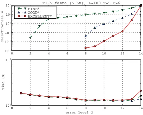
Figure 9 shows the influence of the parameter d on selectiveness and running time for the CFTR dataset with L = 100, r = 5 and q = 6. The running times of FINE*, GOOD*, and EXCELLENT* are comparable: they slightly differ only for d > 10. For low values of d, the selectiveness of GOOD* and EXCELLENT* is 0 (and indeed does not even appear in the figure because of the log scale). The reason is that the divergence of these sequences is bigger than 4%, since they belong to different species. The FINE* filter shows its limits concerning selectiveness since it does keep something (all false positives) also for these low maximal error rates.
We thus focus our attention on large maximal error rates d. Table 3 shows 12 parameter sets with errorsd= 10 (q= 4, 5, 6, 7, 8),d= 12 (q= 4, 5, 6, 7),d= 14 (q= 4, 5, 6). In all cases we haveL= 100 andr= 5. ComparingGOOD* to FINE*,GOOD* always improved the selectiveness (14.7% on average) as we can see in Table 3. Except in two cases, GOOD* was faster thanFINE* (2.9% on average). Clearly on this data, GOOD* is the choice over FINE* even for larger values of q. Comparing EXCELLENT* to GOOD*,
EXCELLENT* always improved the selectiveness (by
111.5% on average). As expected, in all cases,EXCELLENT* introduced a time overhead (9.4% on average). Only for the cased= 14 andq= 6, where the selectiveness was bad (even for EXCELLENT* with 85%), the selectiveness improvement was smaller than the observed slowdown (13% against 54%). Using the data of Table 3 in Figure 8, we can see the behaviour of algorithmsFINE*,GOOD*, andEXCELLENT* whenqchanges. On one hand,EXCELLENT* always improves selectiveness as q is decreased – this behaviour is typical for EXCELLENT* and it is convenient since we can always improve selectiveness if we are willing to pay the extra running time associated with a decreasing of q. On the other hand, both FINE* and GOOD* have a U-like selectiveness curve with a minimal selectiveness (FINE* reached his minimal for q = 6 and GOOD* reached his minimal forq= 5)–this behaviour is also very typical for these methods. Since the running times of the three methods are basically comparable, due to its much better performances in terms of selectiveness, EXCELLENT* is clearly to be preferred for this data set instead ofFINE* and GOOD*.
Applying the filtered sequences to a local multiple aligner
Finally, we discuss the application of TUIUIU* as a preprocessing tool to a local multiple alignment program, using the CFTR data we described earlier. Exact local multiple aligners of k sequences each of lengthntake time proportional to 2k-1nkusing dynamic programming. For this reason, existing multiple aligners provide only a suboptimal solution. The algorithms will still provide a suboptimal solution even when a filter is applied upstream. This is important to observe for what will follow. It means that although TUIUIU* is a lossless filter, the end result may not correspond to the optimal alignment if the aligner itself is a heuristic, or if it is designed to optimise a scoring function different from the one the filter is made for. It may even in some cases lead to a worse alignment score than the one obtained without filtering. Indeed, this is not the best use of a lossless filter, but filters, lossless or not, remain important devices for improving the efficiency and quality of multiple aligners, independent from whether the latter are exact or heuristic, as we shall see in the tests described in this section.
100 101 102 103 104
10−3
10−2
10−1
100
101
102
Selectiveness %
chr22.fa (50M), L=260 d=13 (b=16) q=14
FINE GOOD EXCELLENT
100 101 102 103 104
number of repeats r 102
103
104
Time (s)
Figure 7
Influence of number of repeatsr over selectiveness and running time. Influence of number of repeats rover selectiveness and running time. Human Chromosome 22 with parameters (L, d, r) = (260, 13, r) with q= 14. The selectiveness of 0 obtained for methods GOODandEXCELLENT
are not drawn on the log scale. Asrgrows, the selectiveness decreases because more frequent repeats are rarer than the less frequent ones. Also, variant FINEgets less selective asr
increases. Moreover, this illustrates a case in whichEXCELLENT
is time consuming while not bringing an improvement on the selectiveness with respect to GOODas we could see also in
To our purposes, a local as opposed to a multiple aligner was also a preferable choice to illustrate the use of TUIUIU*. This limited the options, most multiple aligners being global. We decided to use GLAM2 http://bioinfor-matics.org.au/glam2/doc/ which is an evolution ofGLAM (gapless local alignment of multiple sequences, [20]) that was made for multiple alignments without gaps. Differently from its predecessor, GLAM2 allows for gaps
and hence indels. Since the size of the searching space of GLAM2 is nk, GLAM2 samples such space using a Gibbs Sampling method for multiple alignment with simulated annealing for the optimisation step.
We first applied GLAM2 directly on the unfiltered CFTR dataset. It took 34 hours and 55 minutes to run it in order to find the best multiple alignment of the CFTR data. GLAM2 may in fact provide not just one best alignment but the ten best scoring alignments. The top Table 3:FINE/GOOD/EXCELLENTcomparison on CFTR dataset
d q p selectiveness (%) running time(s) GOOD-FINE EXCELLENT-GOOD EXCELLENT-FINE
FINE GOOD Excel FINE GOOD Excel SU SI SD SI SD SI
8 13 13.84 5.10 1.36 123 116 131 1.055 2.71 1.129 3.76 1.070 10.21 7 24 12.85 1.91 0.05 371 370 385 1.003 6.71 1.041 41.90 1.037 281.28 10 6 35 14.28 0.89 0.01 1286 1292 1326 0.995 16.05 1.026 81.23 1.031 1304.19 5 46 21.92 0.65 0.00 5080 5138 5183 0.989 33.95 1.009 235.94 1.020 8011.07 4 57 57.96 1.02 0.00 13441 13362 13564 1.006 56.77 1.015 391.15 1.009 22208.66
7 10 50.85 24.51 13.50 405 382 468 1.059 2.07 1.223 1.81 1.155 3.76 12 6 23 28.09 3.99 0.13 1274 1262 1338 1.009 7.04 1.060 30.37 1.051 214.04 5 36 36.84 2.30 0.04 4972 4952 5055 1.004 16.02 1.021 53.37 1.017 855.33 4 49 85.10 3.53 0.02 13834 13612 13676 1.016 24.08 1.004 162.60 0.988 3916.57
6 11 99.63 96.79 85.71 1609 1405 2159 1.145 1.02 1.536 1.12 1.342 1.16 14 5 26 75.19 12.46 0.35 5017 4794 5080 1.047 6.03 1.060 35.70 1.013 215.46 4 41 99.68 25.08 0.08 14290 13969 14112 1.023 3.97 1.010 299.49 0.988 1190.06
mean 1.029 14.70 1.094 111.54 1.060 3184.32
Measures forFINE/GOOD/EXCELLENTon the CFTR dataset with different parameters sets (L, r = 100,5) with large errorsdand different values ofq. Recall that SD, SU and SI stand forspeed-up,slowdownandselectiveness improvementrespectively.
3.0 3.5 4.0 4.5 5.0 5.5 6.0 6.5 7.0 10−3
10−2
10−1
100
101
102
Selectiveness %
T1−5.fasta (5.5M), L=100 d=12 (b=16) r=5
FINE* GOOD* EXCELLENT*
3.0 3.5 4.0 4.5 5.0 5.5 6.0 6.5 7.0 q−gram size q
102
103
104
105
Time (s)
Figure 8
Influence of q-gram sizeqover selectiveness and running time. Influence of q-gram sizeqover selectiveness and running time for CFTR dataset with parameters (L, d, r) = (100, 12, 5). This test shows thatEXCELLENTis essential
when using a smallq, which enables to filter for a high error rate such as 12%. For instance, withq= 3,EXCELLENTreduces
the selectiveness of 100% observed for bothFINEandGOOD
to 0.01%.
0 2 4 6 8 10 12 14
10−3
10−2
10−1
100
101
102
Selectiveness %
T1−5.fasta (5.5M), L=100 r=5 q=6 FINE*
GOOD* EXCELLENT*
0 2 4 6 8 10 12 14
error level d 103
104
Time (s)
Figure 9
Influence of maximal errordover selectiveness and running time. Influence of maximal errordover