Simulated Annealing based Wireless Sensor
Network Localization
Anushiya A Kannan, Guoqiang Mao and Branka Vucetic
School of Electrical and Information Engineering, the University of Sydney, NSW 2006, Australia. Email:{anushiya,guoqiang, branka}@ee.usyd.edu.au
Abstract— In this paper, we describe a novel localization algorithm for ad hoc wireless sensor networks. Accurate self-organization and localization capability is a highly desirable characteristic of wireless sensor networks. Many researchers have approached the localization problem from different perspectives. A major problem in wireless sensor network localization is the flip ambiguity, which introduces large errors in the location estimates. In this paper, we propose a two phase localization method based on the simulated an-nealing technique to address the issue. Simulated anan-nealing is a technique for combinatorial optimization problems and unlike the gradient search method, it is robust against being trapped into local minima. In this paper we show that our simulated annealing based localization method can be used in ad hoc wireless sensor networks to estimate the location of nodes accurately. In the first phase of our algorithm, simulated annealing is used to obtain an accurate estimate of location. Then a second phase of optimization is performed only on those nodes that are likely to have flip ambiguity problem. Based on the neighborhood information of nodes, those nodes likely to have been affected by flip ambiguity are identified and moved to the correct position. The proposed scheme is tested using simulation on a sensor network of 200 nodes whose distance measurements are corrupted by Gaussian noise. Simulation results show that the proposed novel scheme gives accurate and consistent location estimates of the nodes, and mitigate errors due to flip ambiguity. The performance of the proposed algorithm is better than the performance of some well-known schemes such as DV-hop method and convex optimization based semi-definite programming method.
Index Terms— wireless sensor network, localization, flip ambiguity, simulated annealing
I. INTRODUCTION
Recent advances in integrated circuit design, embedded systems and novel sensing materials have enabled the development of low cost, low power, multi functional sensor nodes. These nodes with wireless interfaces and on-board processing capacity bring the idea of wireless sensor network into reality. It changes the way informa-tion is collected, specially in situainforma-tions where informainforma-tion is hard to capture and observe.
Cheap, smart sensors, networked through wireless links and deployed in large numbers, with automatic localiza-tion capabilities provide unprecedented opportunities in many applications. Some of them include monitoring pa-tients and assisting disabled papa-tients in the health sector;
Part of this paper has been published as a conference paper at IEEE Conference on Local Computer Networks 2005. This paper contains a major modification of the conference paper and it also includes an enhancement of the algorithm presented in the conference paper.
monitoring and controlling homes and cities; monitoring bush fire and water quality surveillance in environmental monitoring applications; monitoring humidity and tem-perature in precision agriculture. In addition, there are a broad spectrum of applications in the defense related area, where smart sensors offer new capabilities for re-connaissance and surveillance as well as other tactical applications.
In a sensor network, there will be a large number of sensor nodes densely deployed at positions which may not be predetermined. In most sensor network applica-tions, the information gathered by these micro-sensors will be meaningless unless the location from where the information is obtained is known. This makes localization capabilities highly desirable in sensor networks. A major problem in wireless sensor network localization based on distance measurements is the flip ambiguity, which introduces large errors in the location estimates. Flip ambiguity occurs when a node’s neighbors are placed nearly collinear, or in the case of erroneous distance measurements.
This paper proposes a two-phase simulated anneal-ing based localization algorithm (SAL), where an initial location estimate is obtained in the first phase using the simulated annealing technique [1] and the large error due to flip ambiguity is mitigated in the refine-ment phase using neighborhood information of nodes. The proposed algorithm is implemented in a centralized architecture, where all nodes send their measurements to a central station for localization. Generally speaking, a distributed architecture will improve scalability and reduce complexity of the algorithm. However in some applications such as monitoring patients and assisting disabled patients in the health sector; monitoring and controlling homes and cities; monitoring bush fire and water quality in the environment; monitoring humidity and temperature in precision agriculture, a central system exists, which gathers information from all nodes hop-by-hop and make decisions accordingly. In such applications where a centralized architecture already exists, it may be more convenient to implement a centralized localization algorithm. The feasibility of nodes communicating their information to a central station has been demonstrated in [2].
section IV describes our proposed SAL approach where subsection IV-A introduces the basic SAL technique and describes the first phase of the proposed algorithm and subsection IV-B talks about the flip ambiguity problem and describes the refinement phase of the proposed al-gorithm; and section V presents simulation results. We conclude this paper in section VI, together with intended future work.
II. RELATEDWORK
Generally, it is assumed that there are a number of anchor nodes in the sensor network. The locations of anchor nodes are known and they are used to fix the local coordinate system. However due to constraints on cost and complexity, most sensor nodes have unknown locations, which are to be estimated with respect to a set of anchor nodes with known location information.
Many researchers have approached the localization problem from different perspectives. Here we focus on localization methods based on distance measurements. But the proposed SAL localization method does not rely on specific distance measurement technique.
A. Distance Measurement
Distance measurements may be obtained by measuring signal propagation time or received signal strength (RSS) information.
Different ways of obtaining signal propagation time include time of arrival (ToA), round trip time of flight (RToF) or time difference of arrival (TDoA) of a sig-nal [3]. Some of these propagation time based measure-ments require very accurate synchronization between the transmitter and the receiver. Furthermore, due to the high propagation speed of wireless signals, a small error in propagation time measurements may cause a large error in the distance measurements.
Since most of the mobile units in the market already have RSS indicator built in them, RSS method looks attractive for range measurements. But the accuracy of this method can be very much influenced by multi-path, fading, non-line of sight (NLoS) conditions and other sources of interference.
B. Coordinate Estimation
In the literature, different approaches are considered for coordinate estimation of the sensor nodes. The main aim of these methods is to estimate the coordinates of the sensor nodes with minimum error.
Niculescu [4] proposed a distributed, hop by hop localization method (APS). It uses a similar principle as that of GPS. Unlike in GPS, not all sensor nodes will have direct communication with anchors in a sensor network. They can only communicate with their one-hop neighbors which are within their transmission range. Long-distance transmission is achieved by hop-by-hop propagation. Each non-anchor node maintains an anchor information table and exchanges updates only with its neighbors. APS method starts with all anchors broad-casting hop counts which are initially set to zero. When
the sensor nodes receive the broadcast, they will update the anchor information table and broadcast it again with hop count increased by one. Once all the anchors have received the distance of the other anchors measured in number of hops, they estimate the average distance for one hop. This information is broadcasted by the anchors as a correction factor to the entire network in hop-by-hop fashion. On receiving the correction factor, a non-anchor node may estimate distances to anchor nodes and perform trilateration to get its estimated coordinate.
Savarese [5] proposed a method which has two phases, HOP-TERRAIN and refinement. The HOP-TERRAIN phase is similar to that of Niculescu’s, allowing all nodes to arrive at initial location estimates. The refinement phase is an iterative algorithm. It uses the results of the HOP-TERRAIN phase and the distance measurements of the immediate neighbors to do the least square trilateration. To mitigate error propagation, a confidence level, which is a value between (0,1), was assigned to each node’s estimated location. Nodes, like anchors, that have high faith in their location estimate select a high confidence value. A node that observes poor conditions (e.g., few neighbors) select a low confidence value. These are used to weigh the equations when solving the system of linear equations and neighbor with a higher confidence value has more impact on the outcome of the trilateration.
Savvides [6] extended the single hop technique of GPS to multi-hop operation as in Niculescu’s thus waiving the line of sight requirement with anchors. Non-anchor nodes collaborate and share information with one another over multiple hops to collectively estimate their locations. To prevent error accumulation in the network, they used least squares estimation with a Kalman filter to estimate locations of all non-anchor nodes simultaneously. In order to ensure that the solution is unique, they used a method called computation trees. To avoid converging at local minima, they used a geometrical relationship to obtain an initial estimate that is close to the final estimate. His algorithm is based on the assumptions that the distance measurements between the nodes and their neighbors are accurate.
Doherty [7] approached the problem using convex optimization based on semi-definite programming. The connectivity of the network was represented as a set of convex localizing constraints for the optimization prob-lem. Pratik [8] extended this technique by taking the non-convex inequality constraints and relaxed the problem to a semi-definite program. Tzu-Chen Liang improved Pratik’s method further by using a gradient-based local search method [9]. All these semi-definite programming methods requires rigorous centralized computation.
Cost
Configurations Current Configuration
Downhill Move
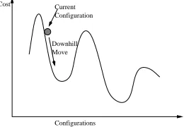
Figure 1. Configuration space: balls and hills.
III. SIMULATEDANNEALINGTECHNIQUE
The theory of simulated annealing originated from the formation of crystals from liquids. The concept is based on the manner in which liquids freeze or metals recrystalize in the process of annealing. Let us consider how to coerce a solid into a low energy state. A low energy state usually means a highly ordered state, such as crystal lattice; a relevant example here is the need to row silicon in the form of highly ordered, defect free crystals for use in semiconductor manufacturing. To accomplish this, the material is annealed: heated to a temperature that permits many atomic rearrangements, then cooled carefully and slowly. As cooling proceeds, the system becomes more ordered and approaches a “frozen” stable state at a low temperature and the material freezes into a good crystal.
In physical chemistry, a low energy state usually means a highly ordered state, such as a crystal lattice; but it is also known that low temperature alone is not a sufficient condition for finding the ground state of the substance. When a substance is heated to a high energy state it permits many atomic rearrangements. If it is cooled in an un-controlled manner allowing the substance get out of equilibrium, it may form a glass or a crystal with defects. But if it is cooled carefully and slowly, allowing it to come to thermal equilibrium at each temperature, it will form a single defect free crystal. This careful controlled cooling procedure was modeled as an efficient technique for a collection of atoms in equilibrium at a given temperature by metropolis [10] in early days.
The simulated annealing algorithm exploits an analogy between the way in which a metal cools and freezes into a minimum energy crystalline structure (the annealing process) and the search for a minimum in a more general system. It is a generalization of the Monte Carlo method. It transforms a poor, unordered solution into a highly optimized, desirable solution. This principle of simulated annealing technique with an analogous set of “controlled cooling” operations was used in the combinatorial op-timization problems, such as minimizing functions of multiple variables, to obtain a highly optimized, desirable solution by Kirkpatrick [11]. The “balls and hills” dia-gram [12] in Fig. 1 illustrates an optimization problem in one dimension. The cost surface is defined by including all the possible values of the cost function f(x), taken over all legal configuration of x. In a normal gradient search method, the current configuration is perturbed only in the direction of reducing cost. Each new perturbation moves to a configuration downhill from the previous
one. This may results in the solution trapped in a local minimum. Simulated annealing allows perturbations to move uphill in a controlled fashion. Because each per-turbation can transform one configuration into a worse configuration, it is possible to jump out of local minima and potentially fall into a more downhill path. However, because the uphill moves are carefully controlled; when we get closer to a good, final solution, we need not worry about getting out of it by an uphill move to some far worse one.
Even though simulated annealing could organize ran-domly placed variables into an optimized meaningful solution, it does not guarantee to get the optimum answer; but will give an acceptable answer in a reasonable time. Obtaining a good estimate for an optimization problem depends on the ability to simulate how the system reaches thermodynamic equilibrium at each fixed temperature in the schedule of decreasing temperatures.
IV. SIMULATEDANNEALING BASEDLOCALIZATION
The location estimation problem has a natural analogy with the simulated annealing algorithm. Consider a sensor network ofmanchor nodes with known locations andn− m sensor nodes with unknown locations. For simplicity, let the nodes lie on a plane such that node ihas location (xi,yi). Initially all the sensor nodes are initialized with random locations (xi,yi) within the boundaries of the sensor network. All the nodes have the ability to measure the distances between them and their one hop neighbors, which impose constraints on the possible values of the estimated coordinates. The measured distance is the true distance between the non-anchor node and its one hop neighbor, together with Gaussian noise describing the uncertainty of the distance measurement. Let us define a graph G = (V(G), E(G)), where V(G) is the set of all nodes in the sensor network and E(G) is the set of all links between one-hop neighbors. If G is a disconnected graph such that a component of G, G1 =
(V(G1), E(G1)) has the vertex set V(G1) which does not have three or more anchors inG1, then all the sensor nodes in the subgraphG1, i.e all members of vertex set V(G1), is non-localizable and they are removed from the localization system.
A. First Phase of the Proposed Algorithm
In the first phase, simulated annealing is used to obtain an accurate estimate of location of the localizable sensor nodes using the distance constraints. Let us define the set Ni as a set containing all one hop neighbors of node i. The localization problem can be formulated as:
min (xi,yi)
m<i≤n n
i=m+1
jNi
( ˆdij−dij)2
CF
(1)
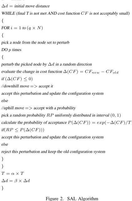
T=initial T
∆d=initial move distance
WHILE (final T is not met AND cost functionCFis not acceptably small)
{
FORi= 1to(q×N)
{
pick a node from the node set to perturb
DOptimes
{
perturb the picked node by∆din a random direction
evaluate the change in cost function∆(CF) =CFnew−CFold
if(∆(CF)≤0) //downhill move=>accept it
accept this perturbation and update the configuration system
else
//uphill move=>accept with a probability
pick a random probabilityRPuniformly distributed in interval(0,1)
calculate the probability of acceptanceP(∆(CF)) =exp(−∆(CF)/T) if(RP≤P(∆(CF)))
accept this perturbation and update the configuration system
else
reject this perturbation and keep the old configuration system
} } T=α×T
∆d=β×∆d }
Figure 2. SAL Algorithm
The cost function CF shown in (1), represents a quantitative measure of the “goodness” of the coordinate estimate. Our aim is to optimize the cost function using simulated annealing technique to get the optimal location estimate without being trapped into a local minimum. The structure of the simulated annealing algorithm is shown in Fig. 2.
When the simulated annealing algorithm initially starts, the system is in a high energy state due to the random initial estimates of the coordinates of the sensor nodes. In each step of the algorithm, a sensor node is chosen sequentially from m+ 1th node to nth node to be per-turbed. The coordinate estimate (xiˆ,yiˆ) of the chosen node iis given a small displacement in a random direction. A new value of the cost function is calculated for the new location estimate. If the change in cost function∆(CF), is less than or equal to zero, i.e.,∆(CF)≤ 0, then the perturbation is accepted and the new location estimate is used as the starting point of the next step.
∆(CF) =CFnew−CFold (2)
The case (∆(CF) > 0) is treated probabilistically: the probability that the displacement is accepted is P(∆(CF)) = exp(−∆(CF)/T). Here T is a control parameter, which by analogy with the SA is known as the system “temperature” and P is a monotonically in-creasing function of T. A random number (RP) uniformly distributed in the interval(0,1)is selected and compared with P(∆(CF)). If it is less than P(∆(CF)) then the perturbation is accepted and the new location estimate is used as the starting point of the next step. Otherwise, the
perturbation is rejected and the original location estimate is kept.
Here temperature T is used as a control parameter to anneal the problem from a random solution to a good, frozen solution. Initially, the “temperature” T is set to a high value to permit aggressive, essentially random search of the configuration space. At a high “temperature” the probability of accepting a large uphill move is high. This could help the system jump out of local minimum. With the increase in the number of iterations, the decrease of system temperature results in decreasing probability of accepting a bad move. The cooling schedule T = α×T, α < 1, is chosen to anneal the problem from a random solution to a good, frozen solution. The idea is to employ a cooling method to moderate the acceptance of uphill moves over the course of the solution. Most of the uphill moves are allowed at higher temperatures. As the temperature cools, fewer uphill moves are allowed. The initial T and the cooling rate α <1 are determined empirically to give a good result. Initial “temperature” was set such that the probability of accepting a bad uphill move is about 80% in the beginning [13].
A move set is a set of allowable perturbation distances that will reach all feasible configurations and it should be easy to compute. Here the move set is chosen to be a random direction in the plane, multiplied by a small distance ∆d in that direction. In order to control the generation of random moves at lower temperatures, we empirically restrict the change in distance as the temper-ature cools by introducing a shrinking factorβ <1, where
∆d=β×∆d.
To get the optimum performance out of the simulated annealing technique, it is necessary to cool carefully and slowly, allowing it to come to thermal equilibrium at each temperature. At each temperature, p× (q × N) perturbations are performed in order to get the system into equilibrium in that particular temperature. Herep is the number of perturbations given to a particular sensor node at a temperature and(q×N)is the number of sensor nodes perturbed at a temperature whereN is the number of nodes in the sensor network andqis a reasonably large number to make the system go into thermal equilibrium. Two criteria can be used to stop the SAL simulation: when the cost function CF is smaller than a predefined small number or when the predefined final temperature is reached.
B. Refinement Phase of the Proposed Algorithm
A B
C
D
E F
G H
I A’ Disc model of node H
Disc model of node I
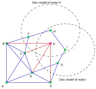
Figure 3. Flip Ambiguity, A solid indicates the two nodes connected by the line can communicate with each other directly.
only. This phenomena of flip ambiguity is discussed in [14]–[16]. But a good method to solve this problem is yet to be found.
In order to address this problem, a second round of optimization is performed only on those nodes that are likely to have flip ambiguity. We should notice in Fig. 3 that the flipped position A’ has gone into the wrong neighborhood of nodes H and I. In a sensor network with a medium to high node density, there is a high chance that a node’s location estimate, which has been flipped, will fall into the wrong neighborhood of other nodes or outside the sensor network boundary. Based on this observation, a second phase of optimization is performed to identify location estimates of nodes which are likely to have been flipped and move them to the correct locations.
Let us define a complement set Ni of the setNi as a set containing all nodes which are not neighbors of node i. IfR is the transmission range of the sensor node and the estimated coordinate of node j ∈ Ni is such that
ˆ
dij < R, then the node j has been placed in the wrong neighborhood of nodei, resulting in both nodes i and j having each other as wrong neighbors. That is, a nodei could be placed into the wrong neighborhood either when the nodeiunder consideration is flipped and moved in to a wrong neighborhood or another node j, which is a member of setNi, has been flipped and estimated to be in setNi. Here a disc model of radiusRaround each node is used to identify the nodes having the wrong neighborhood.
After the first phase of the localization, if a sensor node is in the correct neighborhood then it will be elevated to an anchor node. Refinement phase will not perturb these elevated anchors. If the neighborhood of a sensor node is wrong, it will be identified as non-uniquely localizable node and placed in the set of nodes to be re-localized using the refinement phase. It is worth noting that, when the node density is low, there is possibility for a node to be flipped and still maintain the correct neighborhood. In situations like this, the node will be identified as uniquely localizable and thus elevated erroneously to an anchor node.
Refinement phase is an iterative algorithm, which is used to improve upon and refine the location estimates generated by first phase. Given the initial location esti-mates of the first phase, the objective of the refinement
phase is to identify the non-uniquely localizable nodes, which have either gone outside the boundary or having a wrong neighborhood and perturb them using the basic SAL principles with modified cost function to refine the results. If a node j ∈ Ni have been estimated such that dijˆ < R, then it has been placed in the wrong neighborhood and the minimum error due to the flip is
ˆ
dij −R. The cost function for the refinement phase is modified to include this error term in order to introduce extra cost to a new estimate if it falls into the wrong neighborhood. This will influence the acceptance of the new estimation. This extra term helps push the new estimate away from the wrong neighborhood. With these information, the localization problem in the refinement phase can be formulated as:
min
(xi,yi)
m<i≤n
n
i=m+1
(
jNi
( ˆdij−dij)2+
j∈Ni
ˆ dij<R
( ˆdij−R)2)
CF
(3) The cost functionCF in the refinement phase is different to that used in the first phase of the algorithm. Since the proposed algorithm is implemented in a centralized architecture, it could have access to estimated locations and neighborhood information of all localizable nodes in the system.
In summary, the emphasis for first phase of SAL is to localize the uniquely localizable nodes accurately and give a good starting point to the refinement phase of SAL. Refinement phase of SAL focuses on increasing the accuracy of the localization by optimizing only the non-uniquely localizable nodes with the new cost function.
V. SIMULATIONRESULTS
In order to evaluate the performance of the proposed algorithm, many simulations were performed using visual studio .NET. A sensor network with a total of200nodes is simulated. Sensor nodes are uniformly distributed in a square region of 10×10. All the sensor nodes are initialized with random coordinates within the boundary. The values of p and q in Fig. 2 are chosen as 10 and 2 respectively. The measured distance between the neighboring nodes, which is used in the cost functionCF, is blurred by introducing a Gaussian noise into the true distance as shown in (4).
dij =dt
ij×(1.0 +η×NF) (4) wheredtijanddijare true distance and measured distance respectively between the two nodes i and j.ηis a Gaussian distributed random variable with0 mean and variance1. NF is the noise factor which controls the magnitude of the additionally introduced noise.
TABLE I.
TRANSMISSIONRANGE VS. THECONNECTIVITY
Transmission Range
1.0 1.2 1.4 1.6 1.8 2.0 2.2 2.4 2.6 2.8 3.0
Connectivity 5-6
7-8
10-11
13-14
17-18
20-21
24-27
28-29
33-34
37-39
40-42
0 2 4 6 8 10
0 2 4 6 8 10
X−axis
Y−axis
Location of anchor node
Original location of non−anchor node Estimate location of non−anchor node Error offset between original and estimated location of non−anchor node
Figure 4. Results of first phase with10%Anchors, Transmission range of 1.8 and no Noise.
0 2 4 6 8 10
0 2 4 6 8 10
X−axis
Y−axis
Location of anchor node
Original location of non−anchor node Estimate location of non−anchor node Error offset between original and estimated location of non−anchor node
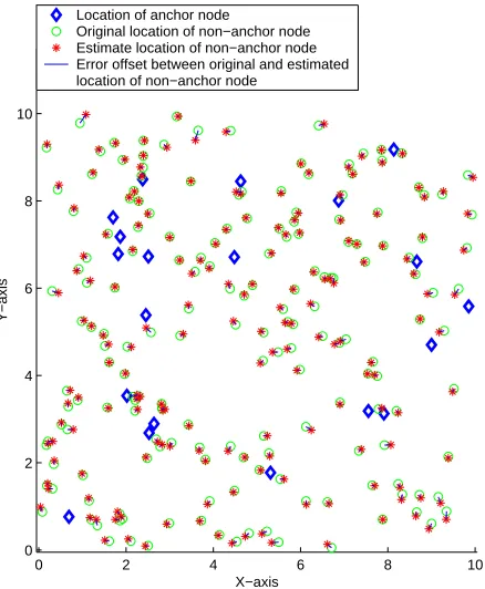
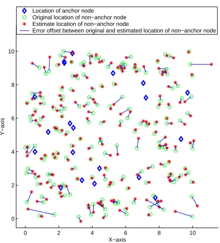
Figure 5. Results of first phase with10%Anchors, Transmission range of 1.8 and10%Noise.
0 2 4 6 8 10
0 2 4 6 8 10 12
X−axis
Y−axis
Location of anchor node
Original location of non−anchor node Estimate location of non−anchor node Non localizable non−anchor node
Neighbors of non localizable non−anchor node Error offset between original and estimated location of non−anchor node
Figure 6. Results of first phase with10%Anchors, Transmission range of 1.8 and10%Noise.
the transmission range is varied in order to vary the connectivity. In Fig. 4 to Fig. 8, the true and estimated sensor locations are shown and an error offset line has been drawn between the true and the estimated locations. Fig. 4 is for the case when there is no error in the distance measurements. Fig. 5 to Fig. 7 shows a location estimate after the first phase of the proposed algorithm and Fig. 8 shows the location estimate after the refinement phase on the result obtained in the first phase shown in Fig. 7.
As shown in Fig. 4, when no noise is introduced, which is an ideal situation, simulated annealing based localization (SAL) estimate the location of the nodes accurately. Fig. 5 shows a SAL simulation results with noise, for10%anchors and a transmission range of 1.8. From this figure we can see that the SAL gives a very accurate result. But this is not the case always. When nodes are placed uniformly, not all non-anchor nodes are uniquely localizable all the time. Most of the nodes which are not uniquely localizable are likely to have the flip ambiguity in their location estimates. Fig. 5 highlights this flip ambiguity situation occurring for a single node. Fig. 7 highlights this flip ambiguity situation occurring for a group of nodes and Fig. 8 shows the location estimate after the refinement phase for the phase 1 results of Fig. 7. It is shown in the figures that the refinement phase mitigates the problem of flip ambiguity and improves the location estimates.
0 2 4 6 8 10 0
2 4 6 8 10
X−axis
Y−axis
Location of anchor node Original location of non−anchor node Estimate location of non−anchor node
Error offset between original and estimated location of non−anchor node
Figure 7. Results of first phase with10%Anchors, Transmission range of 1.3 and10%Noise.
0 2 4 6 8 10
0 2 4 6 8 10
X−axis
Y−axis
Location of anchor node Original location of non−anchor node Estimate location of non−anchor node
Error offset between original and estimated location of non−anchor node
Figure 8. Results of refinement phase with10%Anchors, Transmission range of 1.3 and10%Noise.
simulation results with varying transmission range while having 5% anchor nodes and having 10%anchor nodes respectively. For each point in Fig. 9, ten simulations are performed with different random seeds and the average error is shown. The location error is calculated as in (5). It is reported in percentage, normalized by the transmission range.
location error= 1 (n−m)×
n
i=m+1
(xi−xˆi)2+ (yi−yˆi)2
R2 ×100%
(5)
1.1 1.2 1.3 1.4 1.5 1.6 1.7 1.8 1.9 2 0
50 100 150 200 250
Transmission Range
Location Error (% of Transmission Range)
SAL − 5% Anchor SAL − 10% Anchor SDP− 5% Anchor SDP− 10% Anchor
Figure 9. Location error of uniformly distributed sensor nodes.
where (xiˆ,yiˆ) is the estimated location of sensor node and (xi,yi) is the true location of sensor node.
In SAL when the connectivity is 14 or above, the mean square location error goes below1%, no matter how many anchor nodes are present. As shown in Fig. 9, the proposed algorithm performs much better than SDPL.
VI. CONCLUSION ANDFUTUREWORK
In this paper we presented a novel simulated annealing based localization algorithm which mitigate the flip am-biguity problem. The proposed algorithm is divided into two phases. The first phase uses the simulated annealing technique to obtain an accurate estimate of the nodes’ location. The second phase focuses on the nodes that are likely to have flip ambiguity problem. It uses the neigh-borhood information to identify these nodes and move the nodes to the correct location. Simulations were performed which demonstrated that the proposed algorithm gives better accuracy than the semi-definite programming lo-calization. It was also shown that the proposed algorithm does not propagate error in localization.
The proposed flip ambiguity mitigation method is based on neighborhood information of nodes and it works well in a sensor network with medium to high node density. However when the node density is low, it is possible that a node is flipped and still maintains the correct neighborhood. In this situation, the proposed algorithm fails to identify the flipped node. It is part of our future work to develop a more robust technique to identify nodes that are likely to have flip ambiguity problem.
Still another direction for our future work is inves-tigating implementation of the proposed algorithm in a distributed architecture. This shall improve scalability of the algorithm.
REFERENCES
[2] J. Hill, R. Szewczyk, A. Woo, S. Hollar, D. Culler, and K. Pister, “System architecture directions for networked sensors,” Operatin Systems Review, vol. 34, pp. 93–104, 2000.
[3] M. Vossiek, L. Wiebking, P. Gulden, J. Wieghardt, C. Hoff-mann, and P. Heide, “Wireless local positioning,” IEEE Microwave Magazine, vol. 4, no. 4, pp. 77–86, 2003. [4] D. Niculescu and B. Nath, “Ad hoc positioning system
(aps),” in IEEE GLOBECOM ’01, vol. 5, 2001, pp. 2926– 2931.
[5] C. Savarese and J. Rabaey, “Robust positioning algorithms for distributed ad-hoc wireless sensor networks,” in Pro-ceedings of the General Track: 2002 USENIX Annual Technical Conference, 2002, pp. 317–327.
[6] A. Savvides, H. Park, and M. B. Srivastava, “The bits and flops of the n-hop multilateration primitive for node lo-calization problems,” in International Workshopon Sensor Networks Application, 2002, pp. 112–121.
[7] L. Doherty, K. pister, and L. El Ghaoui, “Convex position estimation in wireless sensor networks,” in IEEE INFO-COM 2001, vol. 3, 2001, pp. 1655–1663.
[8] P. Biswas and y. Ye, “Semidefinite programming for ad hoc wireless sensor network localization,” in Information Processing in Sensor Networks, 2004. IPSN 2004, 2004, pp. 46 – 54.
[9] T. C. Liang, T. C. Wang, and Y. Ye, “A gradient search method to round the semidefinite programming relaxation solution for ad hoc wireless sensor network localisation,” Sanford University, formal report 5, 2004. [Online]. Available: http://www.stanford.edu/ yyye/formal-report5.pdf
[10] M. A. E. . . N.Metropolis, A.Rosenbluth, J.Chem. Phys., 1953.
[11] S. Kirkpatrick, C. D. Gelatt, and M. P. Vecchi, “Optimiza-tion by simulated annealing,” Science, vol. 220, no. 4598, pp. 671–680, 1983.
[12] R. Rutenbar, “Simulated annealing algorithms: an overview,” IEEE Circuits and Devices Magazine, vol. 5, no. 1, pp. 19–26, 1989.
[13] K. Bryan, P. Cunningham, and N. Bolshakova, “Biclus-tering of expression data using simulated annealing.” in CBMS. IEEE Computer Society, 2005, pp. 383–388. [14] D. Moore, J. Leonard, D. Rus, and S. Teller, “Robust
distributed network localization with noisy range mea-surements,” in Second Int. Conf. on Embedded Networked Sensor Systems (SenSys 2004), Nov. 2004.
[15] T. Eren, D. Goldenburg, W. Whiteley, Y. Yang, A. Morse, A. B.D.O, and B. P.N, “Rigidity, computation, and ran-domization in network localisation,” in IEEE INFOCOM 2004, vol. 4, 2004, pp. 2673 – 2684.
[16] D. Goldenburg, W. Krishnamurthy, A.and Maness, Y. Yang, and A. Young, “Network localization in partially localizable networks,” in IEEE INFOCOM 2005, 2005.
Anushiya A Kannan is currently a Ph.D. candidate at the University Of Sydney, Australia in the area of wireless sensor networks. She received her B.Sc and B.E degrees from the Uni-versity of Sydney, Australia, in 1994 and in 1995 respectively. She has worked for TriTech Microelectronics (a member of Singapore Technologies), Singapore, Adaptive Broadband (a spun off from Olivetti Research Lab), Cambridge, UK and Cellonics (a spun off from A*Star), Singapore. Her research interests include wireless sensor networks, wireless communi-cations, ultra wide band and IC design.
Guoqiang Mao received his Master degree in instrumentation engineering from Southeast University, China, in 1998, and the PhD degree in telecommunications from Edith Cowan Univer-sity, Australia, in 2001.
He has worked with a number of industries and academic institutions including Intelligent Pixel Incorporation, University of Wollongong. He became at the School of Electrical and Information Engineering, the University of Sydney, in December 2002. He is currently also a senior researcher at National ICT Australia (seconded staff). His research interests include wireless sensor networks, network quality of service, traffic engineering techniques and wireless communications.
Branka Vucetic received the B.S.E.E., M.S.E.E., and Ph.D. de-grees in electrical engineering from the University of Belgrade, Belgrade, Serbia, in 1972, 1978, and 1982, respectively.