Data Analysis and Statistical Behaviors of Stock
Market Fluctuations
Jun Wang
Department of Mathematics, Beijing Jiaotong University, Beijing 100044, China Email: wangjun@bjtu.edu.cn
Bingli Fan and Dongping Men
Department of Mathematics, Beijing Jiaotong University, Beijing 100044, China
Abstract—In this paper, the data of Chinese stock markets is analyzed by the statistical methods and computer sciences. The fluctuations of stock prices and trade volumes are investigated by the method of Zipf plot, where Zipf plot technique is frequently used in physics science. In the first part of the present paper, the data of stocks prices and trade volumes in Shanghai Stock Exchange and Shenzhen Stock Exchange is analyzed, the statistical behaviors of stocks prices and trade volumes are studied. We select the daily data for Chinese stock markets during the years 2002-2006, by analyzing the data, we discuss the statistical properties of fat tails phenomena and the power law distributions for the daily stocks prices and trade volumes. In the second part, we consider the fat ails phenomena and the power law distributions of Shanghai Stock Exchange Index and Shenzhen Stock Exchange Index during the years 2002-2007, and we also compare the distributions of these two indices with the corresponding distributions of the Zipf plot.
Index Terms—data analysis, statistical methods, Zipf method, statistical properties, computer simulation, market fluctuation
I. INTRODUCTION
The stock prices and the trade volumes play an important role in the market fluctuations in a stock market. In this paper, we focus our attention on the statistical properties of ensembles of the stock prices and the trade volumes. In the first part of the present paper, using 1443 stocks traded in Shanghai Stock Exchange (SHSE) and Shenzhen Stock Exchange (SZSE) during the years 2002-2006, we formed ensembles of daily stock prices and daily trade volumes. The database which used in the present paper is from the websets of Shenzhen Stock Exchange and Shanghai Stock Exchange (www.sse.org.cn, www.sse.com.cn). Considering the history of financial situation of Chinese stock markets, the daily price limit (now 10%), the trading rules of the two stock markets, and the financial policy of Chinese government, we select the data of the daily closing price (for each trading day) for each stock covering the recent 5-year period during the year 2002-2006, the total number of observed data for the stocks prices and the trade volumes is about 2×1443×1205.
In the second part of the present paper, we consider the returns of the fat tails phenomena and the power law distributions of Shanghai Stock Exchange Index and Shenzhen Stock Exchange Index. We select the data for 5 minutes from 9:30 (the opening time of each trading day in China) at February 3, 2002 to 15:00 (the closing time of each trading day) at April 17, 2007. The total number of observed data is 60220 for SHSE index and 60024 for SZSE index. Then we study the statistical properties of returns for SHSE index and SZSE index.
Recently, some research work has been done to investigate the statistical properties of fluctuations of stock prices in a stock market, see [1,2,3,5,6,7,9,10,11]. Their work shows that the fluctuations of price changes are believed to follow a Gaussian distribution for long time intervals but to deviate from it for short time steps, especially the deviation appears at the tail part of the distribution, usually called the fat-tails phenomena. The empirical research has shown the power-law tails in price fluctuations and in trade volume fluctuations. The study on power-law scaling in financial markets is an active topic for physicists to understand the distribution of financial price fluctuations.
In the present paper, Zipf plot method of statistical analysis is introduced to study the market fluctuations. The technique, known as a Zipf plot, is a plot of log of the rank vs. the log of the variable being analyzed. Let
1 2
( ,x x ,L,xN) be a set of N observations on a random variable x for which the cumulative distribution function is F x( ), and suppose that the observations are ordered from the largest to the smallest so that the index i is the rank of xi. The Zipf plot of the sample is the graph of
lnxi against lni . Because of the ranking, 1 ( )i
i N= −F x , so
lni=ln[1−F x( )] lni + N.
its symbol ranking has simple inverse relations, that is
( ) b
P r =cr− . Making a transformation, the above equation can be converted into ln ( )P r =lnc b− lnr , where ( )P r is the frequency of the word whose rank is r. Plotting the graph by ln ( )P r against lnr, the graph is close to a line with the slope of −b. Zipf's law describes that only a few English words are often used, most of the words are rarely used. In recent years, Zipf's law has been widely applied to the literature, computers, networks, management, oil, and many other fields. In the present paper, Zipf plot is applied to study tail phenomena of market fluctuations in the Chinese stock markets, in particularly, the prices of stocks integrated with trade volumes are studied by the statistical analysis.
II. ZIPF PLOT OF QUOTING DATA FROM CHINESE STOCKS PRICES
In this section, we discuss ensemble of 1443 stocks daily prices of Chinese stock markets on September 18, 2006. The theory of statistical method and computer simulation is applied in the following sections, see [4,8,12]. Among these 1443 stocks, denote that the stocks prices in descending order, that is, S(1) is the stock price with the highest price, S(2) is the stock with the second highest price, and S(n) is the n th highest price,
1, ,1443
n= L . Figure 1 is the plot of S(n) against n on a double logarithmic scale, that is the Zipf plot of stocks prices.
0 1 2 3 4 5 6 7 8 -2
-1 0 1 2 3 4 5
log(n)
lo
g
(S
(n
))
β=0.47
Figure 1. Zipf plot of daily prices of 1443 Chinese stocks on September 18, 2006. The horizontal axis shows logarithm of the stocks order
log( )n , the vertical axis shows logarithm of the daily price of stock log( ( ))S n .
In Figure 1, the Zipf plot for the stocks prices higher than 2.72 RMB shows a straight line and is well described by ( )S n ≈n−β with the parameter
0.47
β = ( (n)S ≥2.72). By the similar procedure and analysis, we consider the daily prices of the 1443 Chinese stocks from 2002 to 2006 (totally 1205 trading days in 5 years). We can show that the daily prices of each trading day higher than some threshold value p0 subject to a distribution ( )S n ≈n−β ( (n)S ≥ p0(n)), where the range of the threshold value of the daily parameter β is
0.28<β<0.56. Note that the threshold value p0 depends on the trading dates n.
Figure 2 shows the Zipf plot of the trade volumes of Chinese stocks. In Figure 2, the Zipf plot for the trade volumes higher than 3269000 shows a straight line and is well described by ( )C n ≈n−α with the parameter
=0.77
α ( (n)C ≥3269000) , n=1,L,1443 . By the similar procedure and analysis, we consider the daily trade volumes of the 1443 Chinese stocks from 2002 to 2006 (totally 1205 trading days in 5 years). Similarly, we can show that the daily trade volumes of each trading day higher than a certain threshold value q0 subject to a distribution C n( )≈n−α ( (n)C ≥q0(n)), where the range of the threshold value of the daily parameter α is 0.65<α<1.12.
0 1 2 3 4 5 6 7 8 11
12 13 14 15 16 17 18 19 20
log(n)
log(
C
(n)
)
α=0.77
Figure 2. Zipf plot of daily trade volumes of 1443 Chinese stocks on September 18, 2006. The horizontal axis shows logarithm of the stock
order log( )n , the vertical axis shows logarithm of stock trade
volume log( ( ))C n .
III. THE STATISTICAL CHARACTERS OF PARAMETERS β
AND α
In this section, for each trading day, we discuss the properties of the parameters β and α . The following Figure 3 and Figure 4 show the fluctuations of the values
β and α.
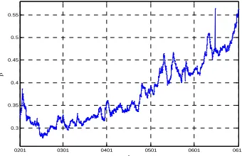
Figure 3. The fluctuations of the power law exponent β in the 5-year
period 2002-2006, corresponding to each trading day. The vertical axis
indicates the power law exponent valueβ , and the horizontal axis
indicates the corresponding trading dates.
Figure 3 shows the movement of the power law exponent β with respect to the trading dates from 2002
0201 0301 0401 0501 0601 0612
0.3 0.35 0.4 0.45 0.5 0.55
t
to 2006, and shows the value range of the parameters β. This can reflect the activity and the trend of Chinese stock markets in large degrees, so this will be helpful for us to understand the status of Chinese macroeconomic. With the reformation and development of Chinese economic systems, the Chinese stock markets develop rapidly, now the movement of stocks prices has a strong influence on the economic behavior of individuals and firms, as a result, it affects the economic development of China directly. In recent years, Chinese stock markets expand quickly, from June 2006 to December 2006, about 65 new companies were listed in Shanghai Stock Exchange and Shenzhen Stock Exchange. According to Zipf-law of five years from 2002 to 2006, the increasing number of Chinese stocks is one of main factors on the increasing trend of parameters β . The other reason of parameters β’s increasing in Figure 3 is that, the degree of the disparity among stocks prices becomes lower as Shanghai Composite Index and Shenzhen Composite Index decline from 2002 to 2003. Shanghai Composite Index and Shenzhen Composite Index are 1643.48 and 3319.21 respectively on January 4, 2002, and 1357.65 and 2759.30 respectively December 31, 2002. Shanghai Composite Index and Shenzhen Composite Index are declined 17.52% and 17.03% respectively in the year 2002. From Figure 3, we can see that the value β fluctuates calmly in 2002. From 2003-2006, Chinese stock markets develop rapidly, Shanghai Composite Index and Shenzhen Composite Index rose by 130%. So in Figure 3, the macro parameters β was increasing, in particularly, the parameter β was substantially increasing in 2006. From above analysis on the parameter
β , this implies that β can reflect the market fluctuations in some scope.
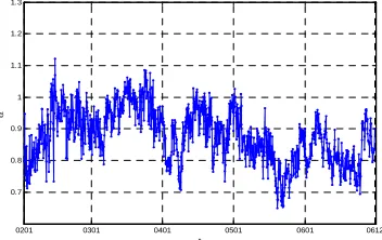
Figure 4. The fluctuations of the power law exponent α in the 5-year period 2002-2006, corresponding to each trading day. The vertical axis indicates the power law exponent valueα , and the horizontal axis indicates the corresponding trading dates.
In the above Figure 4, we consider the movement of the parameter αof the trade volumes by Zipf method. In Chinese stock markets during the years 2002-2006, the fluctuation of the parameter values α is a relatively stable. The degree of the disparity among stocks trade volumes is relatively stable. This implies that the trade volumes of Chinese stock markets had no notable changes from 2002 to 2006.
IV. THE STATISTICAL PROPERTIES OF PARAMETERS β
AND α
In this section, we continue to discuss the statistical properties of the power law exponents β , α defined in above Section 2 and Section 3. The normalized parameters are defined as
' ( )
( )
mean std
β β
β
β
−
= , ' ( )
( )
mean std
α α
α
α
− =
where mean( )β and mean( )α are the means of β and
α respectively, std( )β and std( )α are the standard deviations of β and α respectively. Skewness and kurtosis are the important statistics used to describe the data distributions. Skewness describes the distribution patterns of symmetry. When the value of skewness equals zero, the distribution pattern is symmetric; when the value of skewness is greater than zero, the distribution pattern is positive skewness; and when the value of skewness is less than zero, the distribution pattern is negative skewness. The greater the absolute value of skewness is, the greater the degree of deviation is. Kurtosis is used to describe the steep degree of distribution. If the steep degree of the data distribution is same as that of standard normal distribution, the value of kurtosis equals to 3. When the kurtosis value is bigger than 3, then the steep degree of the distribution is bigger than that of standard normal distribution, the distribution is peak. On the contrary, the distribution is plain. The mathematical definitions of skewness and kurtosis of the vector X =( ,x x1 2,L,xn) are
3 3
1 1
( )
1 n
i i
Skewness x x S n =
= −
−
∑
4 4
1 1
( )
1 n
i i
Kurtosis x x S n =
= −
−
∑
where x is the mean of the vector X =( ,x x1 2,L,xn), and S is the standard deviation of the vector
1 2 ( , , , n) X = x x L x .
TABLE I. PROPERTIES OF THE NORMALIZED PARAMETERS
Minimum maximum skewness kurtosis '
β -1.5 2.83 0.58 2.22
'
α -2.7 2.86 -0.06 2.41
According to the observed trading data of Chinese stock markets, we have Table 1. From Table 1, the skewness value of the parameter β' is 0.58, it is bigger than zero. The distribution of the parameter β' has positive skewness. The value of skewness of the parameter α' is -0.06, close to zero. The values of kurtosis show that, comparing with the normal distribution, the distributions of parameters β', α' are plain. This implies that the statistical distributions of the observed data deviate from the Gaussian distribution in some parts.
0201 0301 0401 0501 0601 0612 0.7
0.8 0.9 1 1.1 1.2 1.3
t
V. THE STATISTICAL PROPERTIES OF PARAMETERS DIFFERENCES
In this section, we continue to study the statistical properties of the parameters βand α , in details that, the properties of the parameters differences ∆β and ∆α . We choose the same markets data in the five years from 2002 to 2006 as in Section 1-4, and let the differences be
1 ,
n n n
β β + β
∆ = − ∆αn =αn+1−αn, for n=1, 2,L,1204. Then the normalized parameters are defined as
' ( )
( ) n
n
mean
std
β β
β
β
∆ − ∆
∆ =
∆ ,
' ( )
( ) n
n
mean
std
α α
α
α
∆ − ∆
∆ =
∆
where mean(∆β) is the mean of ∆β , std(∆β) is the standard deviation of ∆β ,mean(∆α) is the mean of
α
∆ ,std(∆α) is the standard deviation of ∆α.
Next, according to the five years data of Chinese stock markets, we study the cumulative probability distribution of ∆β' and ∆α', that is, P(∆ >β' x), P(∆ >α' x). By the computer simulation, we plot the cumulative probability distributions on the double logarithmic scale, see the Figure 5.
Figure 5. The plot of the cumulative probability distributions of ∆β' and ∆α' under the double logarithmic scale.
From above Figure 5, we can see clearly that the tail distribution of the cumulative probability distribution of
'
β
∆ follows the distribution P(∆ >β' x)≈x−t , (that is the power-law distribution), where t=2.75. The tail of the cumulative probability distribution of ∆α'
also follows the power-law distribution '
( ) t
P ∆ >α x ≈x− , where t=2.19. The values of the exponent parameter t decide the level of the fluctuations of the corresponding parameter differences, the research work on the values of the parameters t is a main part in the study of the fluctuations of the parameters. The smaller the exponent value t is, it means that the more fluctuations the corresponding parameter difference (∆β'
or ∆α' ) has.
In present paper, ∆α'
represents the disparity among the degrees of changes for the trading volumes in each trading day, ∆β'
represents the disparity among the degrees of changes for the stock prices in each trading
day. Figure 5 shows the properties of fluctuations of ∆β'
and ∆α'. This work may help for us to understand the statistical properties of fluctuations in Chinese stock markets.
VI. THE RETURNS OF SHSEINDEX AND SZSEINDEX BY ZIPF PLOT
In this section, according to 5 minutes data from 9:30 at February 3, 2002 to 15:00 at April 17, 2007, we consider the returns of SHSE index and SZSE index by Zipf plot method. China has two stock markets, Shanghai Stock Exchange and Shenzhen Stock Exchange, and the indices studied in the present paper are Shanghai Composite Index and Shenzhen Composite Index. These two indices play an important role in Chinese stock markets. The database is from Shanghai Stock Exchange and Shenzhen Stock Exchange, see www.sse.com.cn and www.sse.org.cn.
For a price time series P t( ), the return r t( ) over a time scale ∆( )t is defined as the forward change in the logarithm of ∆( )t , for t=1,L,n
( ) ln( ( )) ln( ( ))
r t = P t+ ∆ −t P t .
Now we give a new normalized method for the returns of ( )
r t . The following sequence is ordered from the largest value to the smallest one, that is the order statistics
( (1),r L, ( ))r n . Let med r( ) be the median value of the vector ( (1),r L, ( ))r n , and define
R i( )=r i( )−med r( ), i=1, 2,Ln. (1)
On a double logarithmic scale, where R n( )denotes the returns in descending order, R(1) the return with the highest value, R(2) the return with the second highest value, and so on. In the following, we show the comparison of distributions between the returns of SHSE index (SZSE index) and the corresponding normal random variable, here we suppose that the returns and the normal random variable have the same mean and variance.
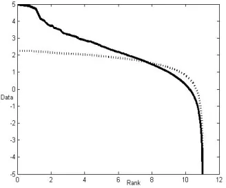
Figure 6. The top curve is a Zipf plot, the double logarithmic plot of returns of SHSE index vs. rank. The bottom curve is a Zipf plot for the corresponding log-normal distribution.
10-1 100 101 10-3
10-2 10-1 100
x
P(
X
>
x)
t=2.19(∆α')
Figure 6 shows the Zipf plot of returns along with the Zipf plot for the log normal. The Zipf plot suggests that the log normal fits the distribution of returns well in some parts. However, in other parts of Figure 6, the Zipf plot makes clear that the returns with the large value are bigger than the corresponding values of log normal, or the Zipf plot of returns lie above the Zipf plot of normal. More specifically, with the aid of Zipf plot, the deviations from the log normal can be seen clearly in Figure 6. First, on the right side of Figure 6, a good fitting distributions can be seen. The main part of deviation is, however, that the tail parts of the distributions on the left side of the graph. This deviation from log normality is statistically significant. From Figure 6, the fat tails phenomena can be seen clearly for the returns of SHSE index, this shows that the distribution of the returns deviates from the Gaussian distribution in the tail parts.
Figure 7 shows the Zipf plot of returns for SZSE index along with the Zipf plot for the log normal. The Zipf plot shows that the two curves separate obviously on the left side of the graph. Figure 7 shows the similar statistical properties of returns for SZSE index as that of returns for SHSE index.
Figure 7. The top curve is a Zipf plot, the double logarithmic plot of returns of SZSE index vs. rank. The bottom curve is a Zipf plot for the corresponding log-normal distribution.
VII. THE EMPIRICAL ANALYSIS OF POWER LAW DISTRIBUTION OF SHSEINDEX AND SZSEINDEX BY ZIPF
PLOT
In this section, for SHSE index and SZSE index, we study the power law distributions of returns sequence { (1),R L, ( )}R n which is obtained by Zipf method, see the definition (1) in Section VI. In order to show the power law distributions of these two Chinese indices, we need to make some adjustment in Figure 6 and Figure 7, that is, we exchange the horizontal axis with the vertical axis. Then applying the theory of linear regression function, we analyze the observed data, further we estimate the coefficient of determination. We are more concerned about that if this linear regression function is a good fit for the observed data, if the returns sequence { (1),R L, ( )}R n follows the power law distribution. In the followings, we give two figures Figure 8 (SHSE index) and Figure 9 (SZSE index) to show the power distribution of returns sequence { (1),R L, ( )}R n .
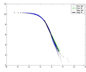
Figure 8. The double logarithmic Zipf plot of rank returns { (1),R L, ( )}R n of SHSE during the years 2002-2007.
By the observed data of Shanghai Stock Exchange during the years 2002-2007, we plot the double logarithmic Zipf plot of rank returns { (1),R L, ( )}R n in Figure 8. The diamond line denotes the positive returns sequence, and the circle line denotes the negative returns sequence. Figure 8 displays that the distributions of the positive returns and the negative returns follow the power law distribution. For the positive returns, the exponent is 0.4279 with the confidence interval of [0.4266, 0.4289], where the significant level is 0.05 . For the negative returns, the exponent is 0.3777 with the confidence interval of [0.3767, 0.3788].
Figure 9. The double logarithmic Zipf plot of rank returns { (1),R L, ( )}R n of SZSE during the years 2002-2007.
CONCLUSION
The objective of this research is to investigate the power law behavior and the fat tails phenomena of Chinese stock markets. Some research work has been done in [5,9] for Chinese stock markets. In this paper, we continue the research work by Zipf plot method.
ACKNOWLEDGMENT
The authors are supported in part by National Natural Science Foundation of China Grant No.70771006, BJTU Foundation No.2006XM044. The authors would like to thank the support of Institute of Financial Mathematics and Financial Engineering in Beijing Jiaotong University, and thank Z. Q. Zhang and S. Z. Zheng for their kind cooperation on this research work.
REFERENCES
[1] J. Elder, A. Serletis, “On fractional integrating dynamics in the US stock market”, Chaos, Solitons & Fractals, vol. 34, pp. 777-781, 2007.
[2] P. Gopikrishnan, V. Plerou, H.E. Stanley, “Statistical properties of the volatility of price fluctuations”, Physical Review E, vol. 60, pp. 1390-1400, 1999.
[3] B. Hong, K. Lee, J. Lee, “Power law in firms bankruptcy”,
Physics Letters A, vol. 361, pp. 6-8, 2007.
[4] K. Ilinski, Physics Of Finance: Gauge Modeling in Non-equilibrium Pricing, John Wiley & Sons Ltd., 2001. [5] M. F. Ji and J. Wang, “Data Analysis and Statistical
Properties of Shenzhen and Shanghai Land Indices”,
WSEAS Transactions on Business and Economics, vol. 4, pp. 33-39, 2007.
[6] T. Kaizojia, M. Kaizoji, “Power law for ensembles of stock prices”, Physica A, vol. 344, pp. 240-243, 2004.
[7] A. Krawiecki, “Microscopic spin model for the stock market with attractor bubbling and heterogeneous agents”,
International Journal of Modern Physics C, vol. 16, pp. 549-559, 2005.
[8] D. Lamberton, B. Lapeyre, Introduction to Stochastic Calculus Applied to Finance, Chapman and Hall, London, 2000.
[9] Q. D. Li and J. Wang, “Statistical Properties of Waiting Times and Returns in Chinese Stock Markets”, WSEAS Transactions on Business and Economics, vol. 3, pp. 758-765, 2006.
[10]T. H. Roh, “Forecasting the volatility of stock price index”,
Expert Systems with Applications, vol. 33, pp. 916-922, 2007.
[11]J. Wang and S. Deng, “Fluctuations of interface statistical physics models applied to a stock market model”,
Nonlinear Analysis: Real World Applications, vol. 9, pp. 718-723, 2008.