Open Access
M E T H O D O L O G Y
Bio
Med
Central
© 2010 Kück et al; licensee BioMed Central Ltd. This is an Open Access article distributed under the terms of the Creative CommonsAttribution License (http://creativecommons.org/licenses/by/2.0), which permits unrestricted use, distribution, and reproduction in any medium, provided the original work is properly cited.Methodology
Parametric and non-parametric masking of
randomness in sequence alignments can be
improved and leads to better resolved trees
Patrick Kück*
1, Karen Meusemann
1, Johannes Dambach
1, Birthe Thormann
1, Björn M von Reumont
1,
Johann W Wägele
1and Bernhard Misof
2Abstract
Background: Methods of alignment masking, which refers to the technique of excluding alignment blocks prior to tree reconstructions, have been successful in improving the signal-to-noise ratio in sequence alignments. However, the lack of formally well defined methods to identify randomness in sequence alignments has prevented a routine application of alignment masking. In this study, we compared the effects on tree reconstructions of the most commonly used profiling method (GBLOCKS) which uses a predefined set of rules in combination with alignment masking, with a new profiling approach (ALISCORE) based on Monte Carlo resampling within a sliding window, using different data sets and alignment methods. While the GBLOCKS approach excludes variable sections above a certain threshold which choice is left arbitrary, the ALISCORE algorithm is free of a priori rating of parameter space and therefore more objective.
Results: ALISCORE was successfully extended to amino acids using a proportional model and empirical substitution matrices to score randomness in multiple sequence alignments. A complex bootstrap resampling leads to an even distribution of scores of randomly similar sequences to assess randomness of the observed sequence similarity. Testing performance on real data, both masking methods, GBLOCKS and ALISCORE, helped to improve tree resolution. The sliding window approach was less sensitive to different alignments of identical data sets and performed equally well on all data sets. Concurrently, ALISCORE is capable of dealing with different substitution patterns and heterogeneous base composition. ALISCORE and the most relaxed GBLOCKS gap parameter setting performed best on all data sets. Correspondingly, Neighbor-Net analyses showed the most decrease in conflict.
Conclusions: Alignment masking improves signal-to-noise ratio in multiple sequence alignments prior to phylogenetic reconstruction. Given the robust performance of alignment profiling, alignment masking should routinely be used to improve tree reconstructions. Parametric methods of alignment profiling can be easily extended to more complex likelihood based models of sequence evolution which opens the possibility of further improvements.
Background
Multiple sequence alignments are an essential prerequi-site in alignment based phylogenetic reconstructions, because they establish fundamental homology assess-ments of primary sequence characters. In consequence, alignment errors can influence the correctness of tree reconstructions [1-3]. To deal with this problem at the level of sequence alignment, different approaches and
alignment software tools have been developed, but despite major advances, alignment quality is still mostly dependent on arbitrary user-given parameters, e.g. gap costs, and inherent features of the data [4,5]. In particular when sequences are highly divergent and/or length vari-able, sequence alignment and the introduction of gaps become a more and more complex enterprise and can currently not be fully governed by formal algorithms. The major problem is that finding the most accurate align-ment parameters in progressive and consistency based alignment approaches is difficult due to the incomplete * Correspondence: [email protected]
1 Zoologisches Forschungsmuseum A. Koenig, Adenauerallee 160, 53113 Bonn, Germany
knowledge of the evolutionary history of sequences and/ or heterogeneous processes along sequences [6]. As a result, problematic sequence alignments will contain sec-tions of ambiguous indel posisec-tions and random similarity. To improve the signal-to-noise ratio, a selection of unambiguous alignment sections can be used. It has been shown that a selection of unambiguously aligned sec-tions, or alignment masking [7], improves phylogenetic reconstructions in many cases [2,8,9]. However, a for-mally well defined criterion of selecting unambiguous alignment sections or profiling multiple sequence align-ments was not available. To fill this gap, different auto-mated heuristic profiling approaches of protein and nucleotide alignments have been developed. GBLOCKS [10] is currently the most frequently used tool. The implemented method is based on a set of simple pre-defined rules with respect to the number of contiguous conserved positions, lack of gaps, and extensive conser-vation of flanking positions, suggesting a final selection of alignment blocks more "suitable" for phylogenetic analy-sis [10,11]. The approach does not make explicit use of models of sequence evolution and is subsequently referred to as a "non-parametric" approach.
The recently introduced alternative profiling method, ALISCORE [12], identifies randomness in multiple sequence alignments using parametric Monte Carlo resa-mpling within a sliding window and was successfully tested on simulated data. ALISCORE was first developed for nucleotide data, but has been extended here to amino acid sequences. The program is freely available from http://aliscore.zfmk.de. In short, within a sliding window an expected similarity score of randomized sequences is generated using a simple match/mismatch scoring for nucleotide or an empirical scoring matrix for amino acid sequences (see Methods), actual base composition, and an adapted Poisson model of site mutation. The observed similarity score is subsequently compared with the
expected range of similarity scores of randomized sequences. Like GBLOCKS it is independent of tree reconstruction methods, but also independent of a priori
rating of sequence variation within a multiple sequence alignment. Because of its explicit use of, although rather simple, models of sequence evolution, ALISCORE can be called a parametric method of alignment masking.
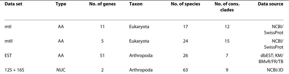
It has been demonstrated that both methods correctly identify randomness in sequence alignments, although to a very different extent [10-12]. A comparison of their per-formance on real data is however missing. Both masking methods suggest a set of alignment blocks suitable for tree reconstructions. These alignment blocks should have a better signal-to-noise ratio and this should lead to bet-ter resolved trees and increased support values. There-fore, we used these predictions to assess the performance of both masking methods by comparing reconstructed Maximum Likelihood (ML) trees. Additionally, our anal-yses compared the sensitivity of tree reconstruction given both profiling approaches in relation to different data and alignment methods. Different test data sets were aligned with commonly used alignment software (CLUSTALX 1.81 [13], MAFFT 6.240 [14], MUSCLE 3.52 [15], T-COF-FEE 5.56 [16], and PCMA 2.0 [17]). For protein align-ments, we used two data sets of mitochondrial protein coding genes that differ in their sequence variability and number of taxa, and an EST data set of mainly ribosomal protein coding genes, including missing data of single taxa. For nucleotide alignments, we tested the perfor-mance of ALISCORE and GBLOCKS on highly variable 12S + 16S rRNA sequence alignments (Table 1).
Results
ALISCORE algorithm for amino acid data
As for nucleotide sequences [12], ALISCORE uses a slid-ing window approach on pairs of amino acid sequences to generate a profile of random similarity between two
Table 1: General overview of used data sets
Data set Type No. of genes Taxon No. of species No. of cons.
clades
Data source
mtI AA 11 Eukaryota 17 12 NCBI/
SwissProt
mtII AA 5 Eukaryota 24 15 NCBI/
SwissProt
EST AA 51 Arthropoda 26 7 dbEST; KM/
BMvR/FR/TB
12S + 16S NUC 2 Arthropoda 63 9 NCBI/JD
sequences. In contrast to the algorithm with nucleotide data, ALISCORE employs the empirical BLOSUM62 matrix, Q, (or alternatives of it, PAM250, PAM500, MATCH) to score differences between amino acids, Qij. Pairs containing indels and any amino acid are defined by using the value of a comparison of stop codons and any amino acid defined within Q. The observed score within a window of pairwise comparisons is generated by sum-ming scores of single site comparisons. Starting from a multiple sequence alignment of length L, sequence pairs (i, j) are selected for which the following procedure is exe-cuted: In a sliding window of size w at position k, a simi-larity score S(k) is calculated comparing positions (i(k),
j(k)), ? k (1, 2, ..., L), using the following simple objective function:
Observed scores are compared to a frequency distribu-tion of scores of randomly similar amino acid sequences with length given by the window size. The generation of randomly similar sequences follows the Proportional model [18], which is an adaptation of a simple Poisson model of change probability, adapted for observed amino acid frequencies, but still assuming that the relative fre-quencies of amino acids are constant across sites:
with Pij (t) as the probability of change from amino acid
i to j, πj the frequency of amino acid j, μ the instantaneous rate of change, and t the branch length/time. Different to the algorithm used with nucleotide sequences in which scores are adapted to varying base composition along sequences and among sequences, the frequency distribu-tion of scores of randomly similar sequences is only pro-duced once for amino acid data. The frequency distribution is generated by: 1) collecting frequencies of amino acids of the complete observed data set, 2) gener-ating 100 bootstrap resamples of this amino acid fre-quency distribution and 100 delete-half bootstrap resamples of each of the 100 complete bootstrap resam-ples, and 3) by using these 10,000 delete-half bootstrap resamples to generate 1,000,000 scores of randomly simi-lar amino acid sequences with length given by the win-dow size. This complex resampling leads to an even distribution of scores of randomly similar sequences. The frequency distribution of randomly similar sequences is used to define a cutoff c(α = 0.95) to assess randomness of the observed sequence similarity within the sliding
win-dow. Matching indels are defined as Qij = c/w. The princi-ple of the comprinci-plete scoring process is described in [12].
Testing performance on real data
Extent of identified randomly similar blocks
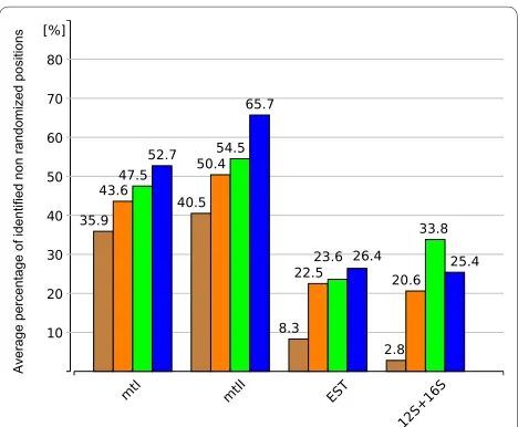
Compared to GBLOCKS, using ALISCORE resulted in the exclusion of fewer positions in most data sets (Figure 1). GBLOCKS identified fewer randomized positions only for the highly diverse 12S + 16S rRNA data with the GBLOCKS(all) option. For each data set, the percentage of identified randomly similar sections differed on aver-age between 1% and 5% for each multiple sequence align-ment when ALISCORE was applied, and between 1% and 9% when GBLOCKS was used. Most alignment sites were discarded by the default option GBLOCKS(none).
ML trees and Neighbor-Net analyses
Resulting ML trees and Neighbor-Net graphs were exam-ined under two different aspects: 1) We compared trees of all unmasked alignments with trees of differently masked alignments per data set to analyze the influence of each masking method on data structure and presence/ absence of selected clades (Figure 2). 2) We compared bootstrap values of corresponding trees (Table 2) and Neighbor-Net graphs (Figure 3) of unmasked and differ-ently masked alignments to see if alignment masking improves the signal-to-noise ratio in the predicted way.
In general, ALISCORE masked alignments resulted in consistent ML topologies among identical but differently aligned sequence data. The ALISCORE algorithm per-formed in most cases better or at least equal well than the best GBLOCKS settings (GBLOCKS(all),
S k Q pij
p k k w
( )= ( )
= + −
∑
1Proportional P t e i j
e i j
ij
j j t
j t
: ( ) ( ) ( )
( ) ( )
= + − =
+ − ≠
⎧ ⎨ ⎪ ⎩
− −
p p
p
m
m
1
1
⎪⎪
Figure 1 Percentage of identified non randomized positions. X-axis: Used data sets. Y-X-axis: Average percentage of "non randomly sim-ilar" positions per data set after alignment masking. GBLOCKS(none): brown; GBLOCKS(half): orange; GBLOCKS(all): green; ALISCORE (blue). A list of all single values is given in the additional file 1.
Table 2: Averaged bootstrap support [%] of selected clades
Data set Selected clades Gb(none) Gb(half) Gb(all) Al Unm
mtI
Plant 63.8 82.0 77.5 81.5 97.0
Viridiplantae 99.8 99.5 99.8 100.0 100.0
Streptophyta 100.0 100.0 100.0 100.0 100.0
(Rhodophyta, Plant)
68.5 92.0 88.5 82.8 96.8
Fungi 100.0 100.0 100.0 100.0 100.0
(Ascomycota, Blastocladiomyco ta)
100.0 100.0 100.0 100.0 100.0
Metazoa 100.0 99.5 99.3 100.0 85.8
Bilateria 93.3 100.0 100.0 100.0 100.0
Gastroneuralia 100.0 100.0 100.0 100.0 100.0
Deuterostomia 73.0 99.8 100.0 99.8 100.0
(Fungi, Metazoa) 100.0 62.5 75.0 76.0 0.0
((Fungi, Metazoa), Amoebozoa)
41.3 17.3 46.3 24.0 0.0
mtII
Plant 0.0 0.0 0.0 0.0 0.0
Viridiplantae 0.0 0.0 0.0 0.0 0.0
Streptophyta 100.0 100.0 100.0 100.0 100.0
Chlorophyta 0.0 0.0 0.0 0.0 0.0
Rhodophyta 99.5 93.5 98.5 97.5 97.8
(Rhodophyta, Plant)
0.0 0.0 0.0 0.0 0.0
Amoebozoa 0.0 0.0 0.0 0.0 14.3
Fungi 100.0 100.0 100.0 100.0 93.3
(Ascomycota, Blastocladiomyco ta)
100.0 100.0 100.0 100.0 96.2
Metazoa 100.0 100.0 100.0 100.0 100.0
Bilateria 100.0 100.0 100.0 100.0 100.0
Gastroneuralia 98.5 100.0 100.0 100.0 88.5
Deuterostomia 69.3 94.5 98.8 95.5 73.3
(Fungi, Metazoa) 87.3 70.5 64.8 79.3 67.5
((Fungi, Metazoa), Amoebozoa)
0.0 0.0 0.0 0.0 0.0
EST
Chelicerata 0.0 50.8 57.5 24.8 0.0
Pancrustacea 97.8 99.5 100.0 100.0 0.0
(Cirripedia, Malacostraca)
GBLOCKS(half )). Application of GBLOCKS(none) yielded less congruent trees.
Amino acid data While plants, fungi, metazoans, and included subtaxa were fully resolved in unmasked trees of data set mtI, sister group relationships between major clades (Fungi, Metazoa, Amoebozoa) could not be resolved without alignment masking. If alignments were masked according to the ALISCORE profile, all ML trees showed a sister group relationship between fungi and metazoans. In the case of the T-COFFEE alignment, the Amoebozoa were placed as sister group to Fungi + Meta-zoa. The alignment masking of GBLOCKS(all) and GBLOCKS(half ) led to comparatively resolved topolo-gies. Masking the alignments with the GBLOCKS(none) option reduced signal in the data (Figure 2). Bootstrap values as measurement of data structure increased after alignment masking, in particular for deep nodes (clade (Fungi, Metazoa) and ((Fungi, Metazoa), Amoebozoa), see Table 2). After alignment masking, Neighbor-Net graphs showed less conflict (Figure 3).
For the mtII data set we were not able to recover mono-phyletic plants and Amoebozoa as sister group to Fungi + Metazoa. The sister group relationship between Fungi and Metazoa was fully resolved in all ALISCORE, GBLOCKS(all), and GBLOCKS(none) masked data sets. GBLOCKS(none) and GBLOCKS(half ) masked align-ments supported in several instances implausible clades (Figure 2).
Bootstrap support values only marginally increased after alignment masking (Table 2). Neighbor-Net graphs
as well showed only marginal reduction of conflicts after alignment masking (Figure 3). Unmasked EST data did not yield well supported resolved trees. Most ALISCORE masked alignments led to clearly improved resolution of 'traditionally' recognized clades (e.g. Chelicerata, Hexapoda, Pancrustacea). If alignments were masked using GBLOCKS(all) or GBLOCKS(half ), tree resolution increased likewise. Using the GBLOCKS(none) masking option did not improve resolution compared to other masked alignments (Figure 2). Considering bootstrap val-ues as measurement of tree-likeness, GBLOCKS(all), GBLOCKS(half ), and ALISCORE improved tree-like-ness of the data (Table 2). Except for the default GBLOCKS(none) setting, Neighbor-Net graphs showed a substantial decrease of conflict after alignment masking (Figure 3).
Nucleotide data Again, ALISCORE and GBLOCKS(all) masking improved tree-likeness of the 12S + 16S nucle-otide alignments at the taxonomically ordinal level. ALIS-CORE outperformed GBLOCKS(all) and GBLOCKS(half ) in all instances. GBLOCKS(none) clearly performed worst (Figure 2, Table 2).
Discussion
Parametric and non-parametric masking methods were successful in identifying 'problematic' alignment blocks. In general, removal of these blocks prior to tree recon-struction improved resolution and bootstrap support. We interprete these results as an improvement in signal-to-noise ratio. For data set mtI and mtII, we assumed clade
Hexapoda 0.0 46.5 66.8 52.8 0.0
Collembola 98.8 99.5 99.8 100.0 0.0
Nonoculata 18.8 74.5 72.8 84.3 0.0
Ectognatha 88.0 55.8 76.8 75.3 0.0
12S + 16S
Campodeidae 17.5 89.3 98.8 97.0 99.8
Diplura 0.0 87.8 96.8 92.5 94.3
Archaeognatha 0.0 59.8 85.3 75.8 47.5
Decapoda 0.0 38.5 38.0 81.8 73.3
Dictyoptera 0.0 38.0 39.3 45.3 49.5
Collembola 0.0 97.5 99.3 97.5 96.0
Odonata 57.8 100.0 100.0 99.3 100.0
Japygidae 29.8 99.5 99.0 100.0 100.0
Hymenoptera 0.0 88.0 84.3 83.8 24.8
Averaged bootstrap support [%] of selected clades of each data set (mtI, mtII, EST, 12S + 16S) inferred from majority rule ML trees for all GBLOCKS profiles (Gb(none), Gb(half), Gb(all)), ALISCORE (Al), and Unmasked (Unm). Values are averaged across different alignment methods per masking approach.
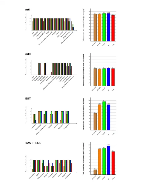
Figure 2 Average percentage of resolved clades within single data sets. On the left: Occurrence of selected clades (Table 2-3) of each data set (mtI, mtII, EST, 12S + 16S), inferred from majority rule ML trees. On the right: Total occurrence of all considered clades [%] for each data set, averaged across all four alignment methods. GBLOCKS(none): brown; GBLOCKS(half): orange; GBLOCKS(all): green; ALISCORE: blue; Unmasked: red.
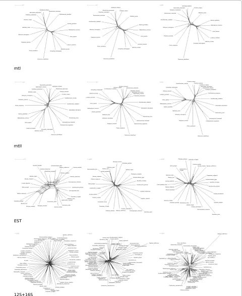
Figure 3 Neighbor-Net graphs. Neighbor-Net graphs generated with SplitsTree 4.10 based on concatenated supermatrices of unmasked (left), ALIS-CORE masked (middle), and GBLOCKS(none) masked (right) data. mtI, mtII and EST networks depend on a T-COFFEE alignment, the 12S + 16S rRNA network on a PCMA alignment. Neighbor-Nets were calculated with uncorrected p-distances. All inferred Neighbor-Net graphs are given in the addi-tional File 1. Tree like structures in these graphs indicate distinct signal-like patterns in the corresponding alignment. Graphs generated from ALISCORE data sets are more tree-like. Lack of information leads to star-like graphs, conflicting signal produces cobwebs.
! ! ! "#"$ "#$ "#$ "#"$ "#$ "#$ % % ! ! & '
! ! & ' ! ! & ' %
"#$ "#"$ "#"$
( ! ) * ( + , % , - &' + ( + + &' - ( % ! , ( + * ) , % , , -) * ! &' - + ( )' $ . % -) /' ( - ' -& & - -) 0 (
) 1 ) $ & 2+ 3*+ 4 ) - $ 1 -
' 3
# )
"#"$ "#"$ "#"$
-2+ $ ) ) & # % ' . $ 1 ( )' /' 4 ( ) 3*+ & ) 1 ) $ ) - 0 - -3 ' & - - ) & # . % ' - - /' ) # - $ ) 5 2+ 3*+ )' ( ( & -4 $ 1 '
validity congruently to Talavera & Castresana [11]. For the EST data set, traditionally accepted clades were only recovered for masked data sets in contrast to the unmasked approach, e.g. Pancrustacea [19-27], Malacost-raca [28-30], Hexapoda [19,20,22,25-27,31-35], Ectogna-tha [22,26,31,32,34,36] or Collembola [22,26,31-35], see Figure 4. A detailed review on these clades including morphological, neuro-anatomical and palaeontological evidence has been recently published in Edgecombe [37] and Grimaldi [38]. An improved data structure after alignment masking is also supported by more distinct split patterns (Figure 3).
Alignment masking further reduced sensitivity of tree reconstructions to different alignment methods. The method implemented in GBLOCKS has the potential to overestimate the extent of divergent or ambiguously aligned positions, especially in partial gene sequences and gappy multiple sequence alignments like EST data or rRNA loop regions. Masking with the GBLOCKS(none) option tended to result in suboptimal node resolution and support values (Figure 2 and Table 2, 3). In the case of the 12S + 16S rRNA data, GBLOCKS(none) masking even reduced signal strength. This phenomenon is clearly evident in Figure 3, where the split decomposition pat-tern appears most fuzzy in the GBLOCKS(none) Neigh-bor-Net graph. We conclude that the incongruence between GBLOCKS(none)- and remaining masked trees may have resulted from conservative and stringent default parameters settings of GBLOCKS, in which all gap including positions were removed and only large served blocks were left. While the higher amount of con-flicting signal in unmasked multiple sequence alignments clearly based on noisy data, it seems that the GBLOCKS(none) masking discarded too many informa-tive positions.
The ALISCORE and GBLOCKS(all) approach per-formed quite similar and best on all data sets. This dem-onstrates that even a predefined set of rules suffices to extract randomness within sequence alignments. Tala-vera & Castresana [11] showed this already in their exten-sive analyses of GBLOCKSs performance. The use of large data sets in phylogenomic analyses resulted in a tre-mendous increase of molecular data, but also in an increase of sampling error which could even bias seem-ingly robust phylogenetic inference [39]. Several such cases have been reported [40-42]. Therefore, it is impor-tant to establish a reliable alignment masking approach to cope with systematic errors in multiple sequence align-ments. Our analyses showed that the sliding window approach will be a useful profiling tool to guide alignment masking.
ALISCORE optionally uses a BLOSUM62 or various PAM matrices to score differences between amino acid sequences, or a simple match/mismatch score for
differ-ences between nucleotide or amino acid sequdiffer-ences. It uses a simple modified Poisson model of character state change (called Proportional for amino acids [18], adapted for uneven base composition and sequence selection) in its resampling procedure to generate a null distribution of expected scores of randomly similar sequences. These scoring models and resampling processes are not very realistic, but however performed well in our analyses.
A recently published alternative approach, NOISY, uses a qnet-graph of sequence relationships to assess random-ness of single positions [2]. The approach uses Monte Carlo resampling of single columns to compare fit of ran-dom data columns on a qnet-graph with the fit of observed data columns. The NOISY method appears as a fast and better alternative to the GBLOCKS approach, but a comparative analyses of its performance with the sliding window approach remains to be done.
Conclusions
We demonstrate for empirical data that alignment mask-ing is a powerful tool to improve signal-to-noise ratio in multiple sequence alignments prior to phylogenetic reconstruction. Masking multiple sequence alignments makes them additionally less sensitive towards different alignment algorithms. Our study also shows, that the scoring algorithm for amino acid data implemented in ALISCORE performs well.
The ALISCORE (parametric) approach is independent of a priori rating of sequence variation and seems to be more capable to handle automatically different substitu-tion patterns and heterogeneous base composisubstitu-tion.
It will be a matter of further analyses, whether an exten-sion of the sliding window approach to more realistic likelihood models of change and Monte Carlo resampling will further improve the performance. However, it would be conceivable to implement a more explicit model based approach in GBLOCKS as well. The advantage of improved parameterizing GBLOCKS could be a signifi-cant gain in speed compared to the sliding window approach. The best approach should be the most efficient one in terms of computational time and increased reli-ability of trees, the latter one admittedly hard to assess.
Methods
Data sets
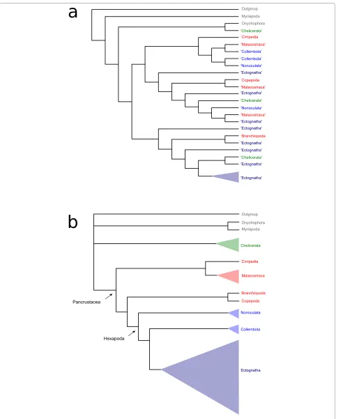
mito-Figure 4 Schematized cladograms inferred from the unmasked and masked EST data set. Schematized cladograms (best ML trees, majority rule) inferred from the T-COFFEE aligned EST data set a) unmasked b) masked with ALISCORE considering selected clades. Quotation marks indicate non-monophyly of clades. Color code: Outgroup (tardigrades), onychophorans, myriapods: grey; chelicerates: green; crustaceans: red; hexapods: blue (proturans, diplurans, collembolans: royal-blue; ectognath hexapods: dark-blue).
chondrial genes of 17 taxa. The second mt data set (mtII) comprised the five less variable genes out of data set mtI but with 24 taxa, corresponding to Talavera & Castresana [11]. The third mitochondrial data set (12S + 16S) included nearly complete 12S + 16S rRNA sequences for 63 arthropod taxa. The nuclear data set (EST) was com-piled from 51 mainly ribosomal protein coding genes from Expressed Sequence Tags (ESTs) of 26 arthropod taxa. These were selected from published (dbEST, NCBI) and unpublished EST data (Meusemann, v. Reumont, Burmester, Roeding, unpubl.). The data set comprised representatives of all major arthropod clades including water bears (Tardigrada) and velvet worms (Ony-chophora). A definitive tree of arthropods has not been established yet, therefore we restricted our comparison on tree resolution and bootstrap support values for selected clades. We remark that increased resolution and support might not reflect a real improvement of phyloge-netic signal-to-noise ratio, but we consider this compari-son as a good approximation in which the bootstrap values are used as approximation of tree-likeness in the data.
Alignments
All genes were aligned separately, each data set using MAFFT 6.240 [14], MUSCLE 3.52 [15], CLUSTALX 1.81 [13], and T-COFFEE 5.56 [16] with default parameters. Since the number of taxa of the rRNA data was too high for T-COFFEE, PCMA 2.0 [17] was used instead which aligns more similar sequences with the CLUSTAL algo-rithm and less similar sequences with the T-COFFEE algorithm. Each alternative alignment was profiled once with ALISCORE and with all three possible gap predefin-itions of GBLOCKS in which either no gaps (GBLOCKS(none)), all gaps (GBLOCKS(all)), or posi-tions which have in less than 50% of sequences a gap (GBLOCKS(half )) are allowed. Thus, five different sets per alignment method were used in tree reconstructions: a) unmasked, b) three different GBLOCKS masked, and c) ALISCORE masked. This was conducted for all four data sets (mtI, mtII, 12S + 16S, EST). Using ALISCORE, alignments were screened separately with 2,000
ran-domly drawn pairwise comparisons and a window size w
= 6. Within its scoring function gaps were treated like ambiguous characters on nucleotide level. On amino acid level we used the BLOSSUM62 substitution matrix. Posi-tions identified by ALISCORE or suggested by GBLOCKS as randomly similar were removed and single genes were concatenated for each data set and each approach. Percentage of remaining positions after mask-ing was plotted for each alignment and maskmask-ing approach (Figure 1), in total for 1,104 single alignments (see addi-tional file 1).
Split Networks
Split decomposition patterns were analyzed with Split-sTree 4 [43], version 4.10. We used the Neighbor-Net algorithm [44] and uncorrected p-distances to generate Neighbor-Net graphs from concatenated alignments of each data set before and after exclusion of randomly sim-ilar sections.
Tree reconstructions
Maximum likelihood (ML) trees were estimated with RAxML 7.0.0 [45] and the RAxML PTHREADS version [46]. We conducted rapid bootstrap analyses and search for the best ML tree with the GTRMIX model for rRNA data and the PROTMIX model with the BLOSUM62 sub-stitution matrix for amino acid data with 100 bootstrap replicates each. Twenty topologies with bootstrap sup-port values of all three GBLOCKS masked, ALISCORE masked, and unmasked alignments were compared for each single data set. Majority rule was applied for all GBLOCKS masked, ALISCORE masked, and unmasked topologies to investigate consistency of selected clades. Clades below 50% bootstrap support were considered as unresolved.
Additional material
Additional file 1 Table S1. Detailed analyses results. Detailed results including lists of the percentage of remained positions after alignment masking per data set and alignment method. Given are all considered clades and corresponding bootstrap values (>50%) per data set, alignment method and (un)masked approach as well as all Neighbor-Net graphs.
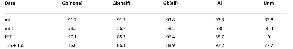
Table 3: Average percentage of resolved clades per data set
Data Gb(none) Gb(half) Gb(all) Al Unm
mtI 91.7 91.7 93.8 93.8 83.8
mtII 58.3 56.7 58.3 60 58.3
EST 57.1 85.7 96.4 85.7 0
12S + 16S 16.6 86.1 88.9 97.2 77.7
Competing interests
The authors declare that they have no competing interests.
Authors' contributions
PK and BM conceived the study, PK designed the setup and performed all anal-yses. PK and BM wrote the paper with comments and revisions from KM, BT, BMvR and JWW. Beta testing of ALISCORE and processing of ESTs was con-ducted by KM. Sequence data was provided by KM (ESTs, hexapods), JD (12S + 16S rRNA), and BMvR (ESTs, crustaceans). All authors read and approved the final manuscript.
Acknowledgements
We gratefully acknowledge the beta testing of the ALISCORE software by Oli-ver Schultz and Julia Schwarzer, which was extremely helpful in identifying bugs. Falko Roeding and Thorsten Burmester kindly provided EST sequences from the milliped Archispirostreptus gigas and the velvet worm Peripatopsis sedgwicki. We thank Michael J Raupach and all members of the molecular and bioinformatic unit of the ZFMK (Bonn) for many inspiring discussions. Work by PK is supported by a doctoral fellowship financed by the DFG, SPP 1174 (WA530/33), which is gratefully acknowledged. BM, KM are and previously JD was supported by the DFG grant MI649/6, JWW is funded by DFG grant WA530/33 and BMvR grant WA530/34.
Author Details
1Zoologisches Forschungsmuseum A. Koenig, Adenauerallee 160, 53113 Bonn, Germany and 2Biozentrum Grindel und Zoologisches Museum, Universität Hamburg, Martin-Luther-King Platz 3, 20146 Hamburg, Germany
References
1. Ogden TH, Rosenberg M: Multiple sequence alignment accuracy and phylogenetic inferrence. Syst Biol 2006, 55(2):314-328.
2. Dress AWM, Flamm C, Fritzsch G, Grünewald S, Kruspe M, Prohaska SJ, Stadler PF: Noisy: identification of problematic columns in multiple sequence alignments. Algorithms Mol Biol 2008, 3:7.
3. Löytynoja A, Goldman N: An algorithm for progressive multiple alignment of sequences with insertions. Proc Natl Acad Sci USA 2005, 102(30):10557-10562.
4. Notredame C: Recent progresses in multiple sequence alignment: a survey. Pharmacogenomics 2002, 3:1-14.
5. Morrison DA: Multiple sequence alignments for phylogenetic purposes. Aust Syst Bot 2006, 19(6):479-539.
6. Nuin PAS, Wang Z, Tellier ERM: The accuracy of several multiple sequence alignment programs for proteins. BMC Bioinformatics 2006, 7:471.
7. Hartmann S, Vision TJ: Using ESTs for phylogenomics: Can one accurately infer a phylogenetic tree from a gappy alignment? BMC Evol Biol 2008, 8(95):S13.
8. Wägele JW, Mayer C: Visualizing differences in phylogenetic information content of alignments and distinction of three classes of long-branch effects. BMC Evol Biol 2007, 7:147.
9. Wong KMA, Suchard MA, Huelsenbeck JP: Alignment uncertainty and genomic analysis. Science 2008, 319(5862):473-476.
10. Castresana J: Selection of conserved blocks from multiple alignments for their use in phylogenetic analysis. Mol Biol Evol 2000, 17(4):540-552. 11. Talavera G, Castresana J: Improvement of phylogenies after removing
divergent and ambiguously aligned blocks from protein sequence alignments. Syst Biol 2007, 56(4):564-577.
12. Misof B, Misof K: A Monte Carlo approach successfully identifies randomness in multiple sequence alignments: a more objective means of data exclusion. Syst Biol 2009, 58:21-34.
13. Thompson JD, Higgins DG, Gibson TJ: CLUSTAL W: improving the sensitivity of progressive multiple sequence alignment through sequence weighting, position-specific gap penalties and weight matrix choice. Nucleic Acids Res 1994, 22(22):4673-4680.
14. Katoh K, Kuma Ki, Hiroyuki T, Miyata T: MAFFT version 5: Improvement in accuracy of multiple sequence alignment. Nucleic Acids Res 2005, 33(2):511-518.
15. Edgar RC: MUSCLE: multiple sequence alignment with high accuracy and high throughput. Nucleic Acids Res 2004, 32(5):1792-1797. 16. Notredame C, Higgins DG, Heringa J: T-COFFEE: A novel method for fast
and accurate multiple sequence alignment. J Mol Biol 2000, 302:205-217.
17. Pei J, Sadreyev R, Grishin NV: PCMA: fast and accurate multiple sequence alignment based on profile consistency. Bioinformatics 2003, 19(3):427-428.
18. Hasegawa M, Fujiwara M: Relative efficiencies of the maximum likelihood, maximum parsimony, and neighbor-joining methods. Mol Phylogenet Evol 1994, 2:1-5.
19. Zrzavý J, Štys P: The basic body plan of arthropods: insights from evolutionary morphology and developmental biology. J Evol Biol 1997, 10(3):653-367.
20. Dohle W: Are the insects terrestrial crustaceans? A discussion of some new facts and arguments and the proposal of the proper name "Tetraconata" for the monophyletic unit Crustacea + Hexapoda. Ann Soc Entomol Fr (New Series) 2001, 37(3):85-103.
21. Richter S: The Tetraconata concept: hexapod-crustacean relationships and the phylogeny of Crustacea. Org Divers Evol 2002, 2(3):217-237. 22. Mallatt J, Giribet G: Further use of nearly complete 28S and 18S rRNA
genes to classify Ecdysozoa: 37 more arthropods and a kinorhynch.
Mol Phylogenet Evol 2006, 3(40):772-794.
23. Harzsch S: Neurophylogeny: Architecture of the nervous system and a fresh view on arthropod phyologeny. Integr Comp Biol 2006, 46(2):162-194.
24. Ungerer P, Scholtz G: Filling the gap between identified neuroblasts and neurons in crustaceans adds new support for Tetraconata. Proc Biol Sci 2008, 275(1633):369-376.
25. Regier JC, Shultz JW, Ganley ARD, Hussey A, Shi D, Ball B, Zwick A, Stajich JE, Cummings MP, Martin JW, Cunningham CW: Resolving arthropod phylogeny: Exploring phylogenetic signal within 41 kb of protein-coding nuclear gene sequence. Syst Biol 2008, 57(6):920-938. 26. von Reumont BM, Meusemann K, Szucsich NU, Dell'Ampio E, Bartel D,
Simon S, Letsch HO, Stocsits RR, Luan Yx, Wägele , Pass G, Hadrys H, Misof B: Can comprehensive background knowledge be incorporated into substitution models to improve phylogenetic analyses? A case study on major arthropod relationships. BMC Evol Biol 2009, 9:119. 27. Mallatt J, Craig CW, Yoder MJ: Nearly complete rRNA genes assembled
from across the metazoan animals: Effects of more taxa, a structure-based alignment, and paired-sites evolutionary models on phylogeny reconstruction. Mol Phylogenet Evol 2009.
28. Richter S, Scholtz G: Phylogenetic analysis of the Malacostraca (Crustacea). J Zoolog Syst Evol Res 2001, 39(3):113-116.
29. Martin JW, Davis GW: An updated classification of the recent Crustacea No. 39 in Science Series, Natural History Museum of Los Angeles County; 2001.
30. Jenner RA, Ní Dhubhghaill C, Ferla MP, Wills MA: Eumalacostracan phylogeny and total evidence: limitations of the usual suspects. BMC Evol Biol 2009, 9:21.
31. Kjer KM, Carle FL, Litman J, Ware J: A Molecular Phylogeny of Hexapoda.
Arthropod Syst Phylogeny 2006, 64:35-44.
32. Kjer KM: Aligned 18S and insect phylogeny. Syst Biol 2004, 53(3):506-514.
33. Luan Yx, Mallatt JM, Xie Rd, Yang Ym, Yin Wy: The phylogenetic positions of three basal-hexapod groups (Protura, Diplura, and Collembola) based on on ribosomal RNA gene sequences. Mol Biol Evol 2005, 22(7):1579-1592.
34. Gao Y, Bu Y, Luan YX: Phylogenetic relationships of basal hexapods reconstructed from nearly complete 18S and 28S rRNA gene sequences. Zoolog Sci 2008, 25(11):1139-1145.
35. Timmermans MJ, D Roelofs D, Mariën J, van Straalen NM: Revealing pancrustacean relationships: Phylogenetic analysis of ribosomal protein genes places Collembola (springtails) in a monophyletic Hexapoda and reinforces the discrepancy between mitochondrial and nuclear DNA markers. BMC Evol Biol 2008, 8:83.
36. Misof B, Niehuis O, Bischoff I, Rickert A, Erpenbeck D, Staniczek A: Towards an 18S phylogeny of hexapods: Accounting for group-specific character covariance in optimized mixed nucleotide/doublet models.
Zoology (Jena) 2007, 110(5):409-429. Received: 9 December 2009 Accepted: 31 March 2010
Published: 31 March 2010
This article is available from: http://www.frontiersinzoology.com/content/7/1/10 © 2010 Kück et al; licensee BioMed Central Ltd.
37. Edgecombe GD: Arthropod phylogeny: An overview from the perspectives of morphology, molecular data and the fossil record.
Arthropod Struct Dev 2009.
38. Grimaldi DA: 400 million years on six legs: On the origin and early evolution of Hexapoda. Arthropod Struct Dev 2009.
39. Nishihara H, Okada N, Hasegawa M: Rooting the eutherian tree: the power and pitfalls of phylogenomics. Genome Biol 2007, 8(9):R199. 40. Blair JE, Ikeo K, Gojoberi T: The evolutionary position of nematodes.
BMC Evol Biol 2002, 2:7.
41. Phillips MJ, Delsuc F, Penny D: Genome-scale phylogeny and the detection of systematic biases. Mol Biol Evol 2004, 21(7):1455-1458. 42. Delsuc F, Brinkmann H, Phillipe H: Phylogenomics and the
reconstruction of the tree of life. Nat Rev Genet 2005, 6(5):361-375. 43. Huson DH, Bryant D: Application of phylogenetic networks in
evolutionary studies. Mol Biol Evol 2006, 23(2):254-267.
44. Bryant D, Moulton V: Neighbor-Net: An agglomerative method for the construction of phylogenetic networks. Mol Biol Evol 2004,
21(2):255-265.
45. Stamatakis A: RAxML-VI-HPC: maximum likelihood-based phylogenetic analyses with thousands of taxa and mixed models. Bioinformatics
2006, 22(21):2688-2690.
46. Ott M, Zola J, Aluru S, Stamatakis A: Large-scale Maximum Likelihood-based Phylogenetic Analysis on the IBM BlueGene/L. Proceedings of ACM/IEEE Supercomputing conference 2007 2007.
doi: 10.1186/1742-9994-7-10
![Table 2: Averaged bootstrap support [%] of selected clades](https://thumb-us.123doks.com/thumbv2/123dok_us/410818.1534070/4.595.64.536.115.734/table-averaged-bootstrap-support-selected-clades.webp)
![Table 2: Averaged bootstrap support [%] of selected clades (Continued)](https://thumb-us.123doks.com/thumbv2/123dok_us/410818.1534070/5.595.61.537.113.324/table-averaged-bootstrap-support-selected-clades-continued.webp)