Characterization of Particle Size Distribution in
Expansive Soils using Logarithmic Density
Distribution
Prof. Charles Lucian
Ardhi University (ARU), P.O. Box 35176, Dares Salaam, TANZANIA
Abstract
Particles size distribution(PSD) is a mathematical function that defines the relative amount, typically by mass, of particles present according to size. Geotechnically, particle size analysis is required torelate soil texture to soil performance or behavior. The objective of this paper is to use a logarithmic scale for particle size to get accurate grain size information for sediment distribution.Through accuratedetermination of grain size, it is possible to examine the influence of particle-size on swelling potential of the soil because chemical composition of sedimentthat relates to swell varies with grain size. Soil samples used in this study were retrieved from open pits in an area which falls within theexpansive soil zone in the Coast Region of Tanzania. The standard analyses used included sedimentation using a hydrometer or pipette method for clay- and silt-sized particles and sieve analysis for sand. For the fact that particle distribution spans over several orders of magnitudes, a basetwologarithmic scalefor the x-axis and a linear scale for the y-axis was used to plot the grain size distribution. The Particle size distribution was supplemented with the free swell tests and Atterbarg Limitsin order to collate Particle size distribution and swell potential. The results showed that the soils have highest sand fractions followed by notable proportion of fines and a small amount of gravel. Ironically, the soils exhibit high swell potential albeit predominance of sand. It implies that expansive character might not be limited to pure clay soils. Hypothetically, sandstones formed by the consolidation of sediments of an expansive nature are likely to have the characteristic to expand.
Keywords: Expansive soils, Particle size, Particle size distribution (PSD), andBase two logarithmic
I. INRODUCTION
The inherent swelling potential of soil is directly related to the total amount of clay-mineral particles (particles that are <2
m in diameter) in it.The swelling potential and swell pressures generated by the swelling of the expansive soil are to a large degree, functions of the combined inherent swelling capacities of all of its clay-mineral components ([7], [15], [16], [22], [24], [26]). The swelling pressureandswelling potential increase with an increase in clay minerals and decreaseas silt, sand, and other non-clay materials increase ([1], [13], [18], [20]). Therefore, separation of sand fractions from silt and clay fractions in the soil may be more important in the study of inherent compositional characteristics of expansivesoils. Soil separation by sieve analysis is a practice or procedure used to assess the particle size distribution(also called gradation).Indeed, soil particle size distribution (PSD)is known to be acritical parameter towardspreliminary understanding of physical and mechanical behavior of soil in many geotechnical applications ([8]). Moreover, particle size distributions of soil mineral separates are critical for getting hold of many soil properties such as water holding capacity, rate of movement of water through the soil, kind of structure of soil, bulk density and consistency of soil. The procedure of determining the size distribution of mineral particles in the soil is called particle size analysis or mechanical analysis of the soil.
[23]).The results of the particle size analysis assist in the soil-classification processes.
Classification of soils for engineering purpose depends very much on the system used. In this study, use is made of the two systems found in [4] and [28]. The grain size and grain size distribution are according to [28], while the wet sieve is according to [4]. That means the distribution of particle sizes larger than 0.002 mm is determined by dry sieve, while a sedimentation process using a hydrometer determines the distribution of particle sizes smaller than 0.002 mm (Fig.1). For both systems, a cumulative frequency distribution graph is plotted for each sample to characterize the relative number of particles within each range of diameter.The graphs are cumulative percent frequency distribution curves, which represent the cumulative weight percent by particle size of the sample. In one of the curves (cumulative weight percent passing), the fraction that is finer than each subsequent grain size is shown. In the other curve (cumulative weight percent retained) the fraction that is coarser than each subsequent grain size is shown. Essentially, for each grain size, the curve indicates how much of the sample is finer or coarser
Particle size distribution in base two logarithmic
In expansive soils, particle diameters typically span many orders of magnitude for natural sediments, thus the best way to conveniently describe wide ranging data set in sediment distribution is the use of base two logarithmic
(phi) scale which allows grain-size data to be expressed in unit of equal values. Logarithmic phi values (in base two) are calculated from particle diameter size measures in millimetres as follows ([21]).
2
log
log
log
10 10 2
d
d
_______________(1)where
= particle size in
units andd
= diameter of particle in mmThe end result is the preparation of particle size distribution curves for soils called cumulative weight percent curves. The cumulative percent frequency distribution curves represent the cumulative-percent mass of each fraction with respect to the total mass of the sample versus the grain-size in mm or phi. Generally, the curves reveal how much of the sample is finer or coarser.
The particle size location and variability can be characterized statistically in terms of mean (average size), standard deviation (the spread/sorting of the sizes around the average), skewness (the degree of asymmetry of the grain sizes around their mean) and kurtosis (degree of the peakedness or flatness of the grains relative to the average) as shown in equations (2) to (14) ([19]). The average grainsizes are measured by mode,mediansize or mean size distribution. The mode or modal diameter (
o)refers to the most frequently occurring particle size in a population ofgrains that corresponds to the diameter represented by thepeakof afrequency curve or steepest point (inflection point) on the cumulative curve. Themedian (
d) size represents the midpoint of thegrain-size distribution and corresponds to the 50% percentile diameter (i.e.50% of the total frequency) on the cumulative curve. Themeansize (m
) is the arithmeticaverageof all the particle sizes in a sample.
m.Clay Silt Sand Gravel Cobble Boulder
Clay Silt Sand Gravel Cobbles Boulders
0.006 0.02
0.002 mm 0.06 mm
0.2 0.6
2 mm 6 20 60 mm 200 mm
Hydrometer
analysis Sieve analysis
Fine-grained soils Coarse-grained soils
The standard deviation is a measure of uniformity or sorting of the sediment represented by a disaggregated sample. Skewness is a measure of the symmetry, or more precisely, the lack of symmetry of the grain size distribution about the mean with a maximum possible value of +1 and a minimum possible value of -1. A positive value of skewness indicates that the distribution has a larger proportion of fine grains and a negative skewness indicates the distribution has a large proportion ofcoarse. A skewness close to zero indicates that the distribution is very symmetrical and themean, median, and mode allfallat the same point. Kurtosis is a measure of the degree of “peakedness/sharpness” or “flatness” of the grain size distribution compared to the normal distribution. Three types of kurtosis that a distribution might display are leptokurtic (relatively peaked distribution; K >1), mesokurtic (normal distribution; K = 1), and platykurtic (relatively flat distribution; K < 1).
avg
x
=
n i i x n 1
1 ___________________________ (2)
s
= 1 1 2 n x x n i avg
i =
1 1 2 2 n x n x n i avg i =
1
1 2 1 2 n n x x n n i n i i i _(3)
C.V =
s
x
avg___________________________(4)Skewness(Skew(X))=
3
1
2
1
n i avg is
x
x
n
n
n
___________(5)Kurtosis (kurt(X)) =
2
3
1 3 3 2 1 1 2 1 4
n n
n s x x n n n n n n i avg i _(6)
where
n
= number of occurrencei
x
= mid point of each class interval in metricavg
x
= mean grain sizes
= standard deviationC.V = coefficient of variation (uniformity of distribution)
According to [3] the alternative to the above statistical formulae is given by Folk and Ward in 1957 in (original) graphical measures in phi (Table I) as follows:
3
84 50
16
m
___________________(7)s
=6
.
6
4
5 95 1684
_____________(8)
Skewness (Sk) =
95 5
50 95 5 16 84 50 84 16
2
2
2
2
_______ (9)Kurtosis (K)=
25 75
5 95
244
___________(10)
where
x = the grain diameter in phi units at thecumulative percentile value of x
m
= mean grain sizeThe modification of the above measures is given in metric in Table II ([3]) as follows:
3 ln ln ln
exp P16 P50 P84
Pm ___________ (11)
s
6 . 6 ln ln 4 ln lnexp P16 P84 P5 P95 ____ (12) Skewness(Sk) =
25 5
50 95 5 16 84 50 84 16 ln ln 2 ln 2 ln ln ln ln 2 ln 2 ln ln P P P P P P P P P P _(13) Kurtosis (K)=
25 75
95 5 244 ln ln P P ______________ (14)
where
P
x is the grain diameter andP
m is the mean in metric unitsI. TABLE I: Description of limits of distribution of values – logarithmic (origin) graphical measures ([21]).
Mean in phi Standard deviation in phi
Skewness Kurtosis
-12 to -8 boulder under .35 very well sorted
from +1.00 to +0.30
strongly
fine skewed under 0.67 very platykurtic
-8 to -6 cobble 0.35-0.50 well sorted from +0.30 to
+0.10 fine skewed 0.67-0.90 platykurtic
-6 to -2 pebble 0.50-0.71 moderately well sorted
from +0.10 to -0.10
near
symmetrical 0.90-1.11 mesokurtic
-2 to -1 granular 0.71-1.0 moderately sorted
from -0.10 to -0.30
coarse
skewed 1.11-1.50 leptokurtic
-1 to 0.0 very
coarse 1.0-2.0 poorly sorted
from -0.30 to -1.00
strongly
grained skewed
0.0 to 1.0 coarse
grained 2.0-4.0
very poorly sorted
- -
over 3.00 extremely leptokurtic
1.0 to 2.0 medium
grained over 4.0
extremely poorly sorted
-
- - -
2.0 to 3.0 fine
grained - -
-
- - -
3.0 to 4.0 very fine grained
- -
-
- - -
5.0 to 6.0 medium
silt - -
-
- - -
6.0 to 7.0 fine silt - - - -
7.0 to 8.0 very
fine silt - -
-
- - -
>8.0 clay - - - -
II. TABLEII: Description of limits of distribution of values – geometric (modified) graphical measures in metric ([3]).
Standard deviation Skewness Kurtosis
<1.27 very well sorted from -0.3 to -1.0 very fine
skewed < 0.67 very platykurtic 1.27 – 1.41 well sorted from -0.1 to -0.3 fine skewed 0.67-0.90 platykurtic
1.41 –1.62 moderately well
sorted from -0.1 to +0.1
near
symmetrical 0.90-1.11 mesokurtic 1.62-2.0 moderately sorted from 0.1 to 0.3 coarse skewed 1.11-1.50 leptokurtic
2.0-4.0 poorly sorted from +0.3 to +1.0 very coarse
skewed 1.50-3.00 very leptokurtic
4.0-16.0 very poorly sorted - - > 3.00 extremely leptokurtic
> 16.0 extremely poorly sorted
- -
- -
I. MATERIALS AND METHODS
A. Study site
The study area (Kibaha) is a township located in eastern Tanzania, about 40 km west of Dar es Salaam (the commercial capital city of Tanzania), along the Dar Es Salaam-Morogoro highway. It’s positioned at an altitude of about 155 m above sea level and located approximately by geographic latitude and longitude of 06º46'S and 38º55'E respectively. It is within the coastal belt where plastic clay soil is predominant.
The geology of the catchment is complex ([14]): it comprises a complex autochthonousand allochthonous sequence of late mesozoic and early cenozoic sediments. The indigenous and non-indigenous sediment fillings are composed of lacustrine, fluviatile, residual, pluvial and alluvial deposits that include micaceous materials (micaceousschists, clay shale, siltstones, silty mudstones etc), calcareous sandstones, limestones, marine marls, shells, organic materials and
conglomerates. By the processes of chemical and physical weathering, these conglomerates converted to soils rich in clay. Typically, the deposits are reddish brown, grey brown and grey in colour. Generally, soils tend to be sandy clay, although deposits of terrace gravels, marine clays and fossiliferous shells are common locally. The underlying basement consists of the crystalline and metamorphic rocks of the Mozambique orogenic belt ([17]). Largely, the soils reflect the geology and climatic conditions of the area.
degree of expansiveness is proportional to the amount of montmorillonite or other expansive clay minerals present in the soil.
B. Soil sampling and analysis
The expansive soilsamples used in this study were retrieved from open pits near Tumbi Catholic Church in Kibaha Town, Coast Region, Tanzania.The retrieved samples were carefully packed in thick polyethylene bags, sealed with tape, logged and transported to thesoil laboratory at the Dar es Salaam Institute of Technology (DIT). At the laboratory, the samples were air-dried, gently crushed, and then dry-sieved using a 2-mm mesh to remove coarse fragments. The samples were then treatedwith an excess of 30% hydrogen peroxide to remove the organicmaterials. Thereafter, the grading analyses were performed using both standard wet-sieve (sedimentation technique) and hydrometer methods. To carry out the two methods, the samples were first washed through 0.063mm sieve, thus the soil passing the sieve was allowed to stand overnight and the suspension was then tested using sedimentation technique (hydrometer). The sedimentation technique is based on an application of Stokes'law to a soil/water suspension and periodic measurement of the density of the suspension. The soil that remained in the sieve was oven dried and subjected to dry sieve in accordance with [4]Methods of test for soils for civil engineering purposes.
C. Dry Sieve Analysis.
Particle size (sieve analysis) carried out for soil classification in accordance with [4]Methods of test for soils for civil engineering purposes allowed the sample retained on the sieve 0.063mm to run run through a standard set of sieves on a mechanical sieve shaker. This partitioned the sample into various grain sizes that allowed presentation of the grain size distribution shown in Table III. The particle size distribution was carried out together with the Atterberg limits (liquid, plastic and shrinkage limits) and hydrometer tests according to the guidelines provided in [4], clause 9.5, density determination based on the standard method for measuring particle density according to [4] clause 7, swell potential, free swell according to [11]and oedometer tests were performed.
D. Wet sieve and hydrometer test
Wet sieving and hydrometer tests were performed to obtain the grain size distribution of fine particles. As it has been pointed out before, the tests
were performed according to the guidelines given in [4] Part 2, clauses 9.2 & 9.5.
The representative test samples were crushed, placed in an evaporating dish and dried overnight in an oven maintained at 105-110°C. The cool dried samples were weighed to the nearest 0.01 g and sieved through a 20 mm sieve. A mass of 2 kg of particles finer than 20 mm was taken to form a number of portions. A portion of 40 g soil was spread in a tray and treated with distilled water and a dispersant solution of 2 g/l sodium hexametaphosphate (known commercially as Calgon) to make 1000 ml. The mixture was stirred for 1 hour to break down and separate clay particles. The soil in small batches was separated into coarser and finer portions by washing it through the 63 µm sieve. The > 63 µm portions were oven dried at 105-110°C and sieved through standard mesh sizes between 20 mm and 63 µm using the dry sieve procedure. The weight retained on each sieve was noted.
The <63 µm portion was mixed with water in a 1000 ml sedimentation cylinder, thoroughly stirred, allowed to settle for about five minutes prior to the decantation of the suspension. The test is an application of Stoke’s law (larger particles fall more quickly in a suspending fluid, while finer particles remain in suspension longer). The reading on the hydrometer determines the amount of that size, while the time at which the hydrometer readings are taken determines the size of particle remaining in suspension. The process was repeated several times to separate particles of different size from each other in the mixed suspension.
E. Free Swell test and Atterberg Limits
Values of 100% or more are associated with clay which could swell considerably, especially under light loadings.
The percent of free swell is expressed in equation (15) as:
Free swell percent = ΔV/V*100% ____________(15) where ΔV =Vs-V= change in initial volume (V) of a specimen and
V = initial volume (10 mm3) of the specimen Vs = final volume of the specimen
II. RESULTS
The results of three samples (RC1, RC2 and RB) from a depth of 1 m of each peat are presented in Tables III&IVand Fig.2. According to [6], soils containing appreciable quantities of colloidal
particles (less than 0.001 mm in diameter) greater than 28% have very high degree of expansion. Soils containing 23% – 15% have medium to high degree of expansion while those containing colloidal particles less than 15% have low degree of expansion. The soils under consideration have very high degree of expansion.
The Particle size distribution was supplement with the free swell tests according to [11]. The test results yielded free swell values between 100% and 150% (Table 3). The results were prima facie evidence that the soils are associated with clay, which could swell considerably when wetted. The soils proved to have the ability to absorb and retain a great deal of water and undergo significant volumetric changes with moisture fluctuations (i.e. clay having high to very high swelling-shrinkage potential)
III. TABLEIII: Physical properties of Kibaha clay samples at the regional office block (RB) and Roman Catholic Church (RC).
Sample No:
Depth (m)
Grain size (%)
Atterberg’s limits (%)
Clay content % (<2µm)
Free swell (%)
Activity Eqn. 2.17
Gravels Sand Fines LL PL PI SL
RC1
0.6 11 50 39 64 21 43 12.5 34 150 1.5
1.0 14 51 35 63 24 39 13.3 30 130 1.6
2.0 16 51 33 54 23 31 14.2 29 100 1.3
3.0 5 59 36 59 22 37 14.0 33 130 1.4
RC2
1.0 9 42 49 69 23 46 11.1 29 140 2.0
2.0 12 63 24 61 30 31 16.6 22 100 1.8
3.0 1 67 32 69 23 46 13.6 27 100 2.0
RB
1.0 2 55 44 51 21 30 16.5 39 130 0.9
2.0 1 60 39 51 15 36 15.0 35 120 1.2
3.0 3 52 44 49 23 26 15.1 34 140 0.9
Mean 7.4 55.0 37.5 59.0 22.5 36.9 14.2 31.2 124.0 1.46
St. Error 1.8 2.3 2.3 2.4 1.2 2.2 0.5 1.5 5.8 0.13
STD 5.7 7.3 7.1 7.4 3.7 6.8 1.7 4.8 18.4 0.40
Kurtosis -1.8 -0.2 0.2 -1.5 3.4 -1.4 -0.1 0.4 -1.3 -1.05 Skewness 0.2 -0.0 -0.2 0.0 0.0 0.1 -0.2 -0.4 -0.3 0.02
Min. 1.0 42 24 49.0 15.0 27.0 11.1 22.0 100.0 0.88
Max. 16 67 49 69.0 30.0 47.0 16.6 39.0 150.0 2.05
IV: TABLEIV: Hydrometer results for samples RC1, RC2 and RB.
RC1 RC2 RB
Particle diameter (D micro-mm)
% finer than D
Particle diameter (D micro-mm)
% finer than D
Particle diameter (D micro-mm)
% finer than D
0.0630 42 0.0649 35 0.06202 45
0.0449 40 0.0459 35 0.04420 43
0.0317 40 0.0327 34 0.03149 42
0.0226 39 0.0231 34 0.02227 42
0.0161 37 0.0163 34 0.01575 42
0.0118 35 0.0119 34 0.01150 42
0.0060 34 0.0060 34 0.00579 40
0.0042 34 0.0042 32 0.00410 40
0.0030 31 0.0030 31 0.00292 39
0.00124 29 0.00125 27 0.00120 37
Fig.2: Hydrometer results for samples RC1, RC2 and RB from 1 metre deep.
RC1 Depth 1.0
0 10 20 30 40 50
0,0010 0,0100 0,1000 1,0000
Particle Diameter, D (mm)
%
f
in
e
r
th
a
n
D
RC2 Depth 1m
0 10 20 30 40
0,0010 0,0100 0,1000 1,0000
Particle diameter, D (mm)
%
f
in
e
r
th
a
n
D
RB Depth 1m
0 10 20 30 40 50
0,00100 0,01000 0,10000 1,00000
Particle Diameter, D (mm)
%
f
in
e
r
th
a
n
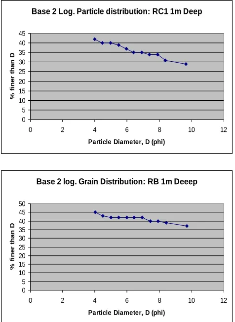
The logarithmic (origin) graphical measures for three samples from a depth of 1 m from each trial pit were calculated according to equation (1) and the results are presented in Fig. 3.
Particles size distribution tests indicated that the soils have highest sand fractions followed by notable proportion of fines and a small amount of gravel (Fig. 3). Ironically, the soils exhibit high swell potential albeit predominance of sand. It implies that expansive character might not be limited to pure clay soils. Hypothetically, sandstones formed by the consolidation of sediments of an expansive nature are likely to have the characteristic to expand.
For the 3 pits, the mean was between 0.0 phi and 1.0 phi, the standard deviation was under 0.5 phi, the skewness ranged from -0.1 to 0.1 and the kurtosis was under 0.67 (equations 5 to 14). Therefore, the soils are coarse grained, very well sorted, nearly symmetry and very platykurtic (Tables 1 & 2).
The coarse grains reflect the presence of terrace gravel deposits and high proportion of sands in the soils. This system allows interpretation of many geological engineering soils rather than geotechnical interpretation. However, the system is in total agreement with [2]: clause 13.1 that the soil is coarse grained if it contains less than 50% fines.
Fig. 3: Base two logarithmic particle size distribution curves for 3 samples.
IV. CONCLUSIONS
In this study the base two logarithmic
(phi) scaleshas been used to represent grain sizeinformation for Particle size distribution(PSD). Sieve size analysis was performed on expansive soil samples and the cumulative distribution curves that represent the cumulative weight percent by particle
Base 2 Log. Particle distribution: RC1 1m Deep
0 5 10 15 20 25 30 35 40 45
0 2 4 6 8 10 12
Particle Diameter, D (phi)
%
f
ine
r
tha
n
D
Base 2 log. Particle Distribution: RC1 1m Deep
0 5 10 15 20 25 30 35 40
0 2 4 6 8 10 12
Particle Diamater, D (phi)
%
f
ine
r
tha
n
D
Base 2 log. Grain Distribution: RB 1m Deeep
0 5 10 15 20 25 30 35 40 45 50
0 2 4 6 8 10 12
Particle Diameter, D (phi)
%
f
ine
r
tha
n
size of the sample werecreated from the analysis data. Indeed the logarithmic scale for particle size has been used to get accurate grain size information for sediment distribution. How much of the sample was finer or coarser has been clearly shown in the cumulative distribution curves.The accurate completion of the sieve-analysis test produced the percentage of different grain sizescontained within a soil that are related to the swelling potential of the soil because swelling potential increases withincreasing fines content. The results showed that the soils have highest sand fractions followed by notable proportion of fines and a small amount of
gravel. Ironically, the soils
exhibitpronouncedswelling-shrinkingbehavior as well ashighplasticity and cohesionalbeit predominance of sand ([14]). It implies that expansive character might not be limited to pure clay soils but also to clay/silt/sand mix. Hypothetically, sandstones formed by the consolidation of arenaceous and argillaceoussediments of expansive nature are likely to have the characteristic to expand.
V. REFERENCES
[1] Abd-Allah, A. M. A., Dawood, Y. H., Awad, S. A. and Agila, W. A. (2009). Mineralogical and Chemical Compositions of Shallow Marine Clays, East of Cairo, Egypt: A Geotechnical Perception. JKAU; Journal of Earth Science, Vol. 20 No.1, pp: 141-166.
[2] ASTM D 2488-00 (2000). Standard practice for description and identification of soils (Visual-manual procedure).
Designation D 2488-00, American Society for Testing Materials, West Conshohocken, PA
[3] Blott, S. J. and Pye, K. (2001). GRADISTAT: a grain size distribution and statistics package for the analysis of unconsolidated sediments. Earth Surface Processes and Landforms, vol. 26, pp. 1237-1248.
[4] BS 1377-2 (1990). Methods of Test for Soils for Civil Engineering Purposes: part 2: Classification tests. British Standard Institution, London.
[5] Centeri, C., Jacab, G., Szabo, S., and Biró, Z. (2015). Comparison of particle-size analyzing laboratory methods.
Environmental engineering and management journal. Vol. 14, No. 5, pp. 1125-1135
[6] Chen, F. H. (1988). Foundations on expansive soils, Elsevier Science Publishers B. V.
[7] Dafalla, M. A. (2017). Advances in Materials Science and Engineering. Advances in Materials Science and Engineering. Vol. 2017 (2017), Article ID 3181794, 9 pages [8] Erguler, Z. A. (2016) A Quantitative Method of Describing Grain Size Distribution of Soils and Some Examples for its application. Bulletin of Engineering Geology and the Environment, Vol. 75, Issue 2, pp. 807 – 819.
[9] Glendon, W. G. and Dani, O. (2002). The Solid Phase-Particle Size Analysis. In: Methods of Soil Analysis. Part 4. Physical Methods, Dane, J.H. and C. Topp (Eds.). Soil Science Society of America, Madison, WI., ISBN-13: 978-0891188414, pp: 255-278.
[10] Guy, H. P. (1969). Laboratory Theory and Methods for Sediment Analysis, ch. C1 (US Geological Survey Techniques of Water-Resources Investigations).
[11] Holtz, W. G. and Gibbs, H. J. (1956). Engineering properties of expansive clays. Transactions, American Society of Civil Engineers, vol. 121, pp. 641-677.
[12] Kettler, T. A., Doran, J. W. and Gilbert T. L. (2001). Simplified Method for Soil Particle-Size Determination to Accompany Soil-Quality Analyses. Soil Science Society of America Journal. Vol. 65, pp. 849–852.
[13] Louafi, B. and Bahar, R. (2012). SAND: An Additive for Stabilzation of Swelling Clay Soils. International Journal of Geosciences, Vol. 3, pp. 719-725.
[14] Lucian, C. (2008). Geotechnical Aspects of Buildings on Expansive Soils in Kibaha, Tanzania. PhD. Thesis in Soil and Rock Mechanics, Royal Institute of Technology (KTH),
Sweden.
http://kth.diva-portal.org/smash/record.jsf;jsessionid=5cf2dfee91b3a0141d fb955e8d17?pid=diva2:37732
[15] Mahamedi, A. and Khemissa, M. (2015),Stabilization of an expansive overconsolidated clay using hydraulic binders.
Housing and Building National Research Center (HBRC) Journal, Vol. 11, Issue 1, pp. 82–90.
[16] Mokhtari, M. and Dehghani, M. (2012). Swell-Shrink Behavior of Expansive Soils, Damage and Control. The Electronic Journal of Geotechnical Engineering (EJGE ), Vol. 17, pp. 2673 – 2682.
[17] Mpanda, S. (1997). Geological development of the East Africa coastal basin of Tanzania.Stockholm contributions in Geology, Stockholm University, Department of Geology and Geochemistry, Stockholm, Sweden.
[18] Mohammed Y. Fattah, Nahla M. Salim, and Entesar J. Irshayyid (2017). Influence of soil suction on swelling pressure of bentonite-sand mixtures. European Journal of Environmental and Civil Engineering. pp. 1-15
[19] Okeyode, I. C. &Jibiri, N. N. (2013). Grain Size Analysis of the Sediments from Ogun River, South Western Nigeria.
Earth Science Research; Vol. 2, No. 1; pp. 43 – 51. [20] Paj¥k-Komorowska, A. (2003). Swelling, expansion and
shrinkage properties of selected clays in the Mazowsze province, central Poland. Geological Quarterly, Vol. 47, No. 1, pp. 55–62.
[21] Pfannkuch, H. O. and Paulson, R. (2005). Grain Size Distribution and Hydraulic Properties.
http://www.cs.pdx.edu/~ian/geology2.5.html. Date of access: 1st September 2016.
[22] Pino, A., Pedarla, A., Puppala A, and Hoyos, L. R. (2016). Evaluation of swell behaviour of expansive clays from specific moisture capacity. E3S Web of Conferences 9, pp. 1 - 5
[23] Rawle, A. (2002). The importance of particle sizing to the coatings industry Part 1: Particle size measurement.
Advances in Colour Science and Technology, Vol. 5, No. 1, pp. 1 - 12
[24] Schanz, T. and Elsawy, M. B. D. (2015). Swelling Characteristics and Shear Strength of Highly Expansive Clay-Lime Mixtures: A comparative Study. Arabian Journal of Geosciences. Vol. 8, Issue 10, pp. 7919 – 7927. [25] Segal, E., Shouse, P. J., Bradford, S. A., Skaggs, T. H. and
Corwin, D. I. (2009). Measuring Particle Size Distribution Using Laser Diffraction: Implications for Predicting Soil Hydraulic Properties. Journal of Soil Science. Vol. 174, No. 12, pp. 639 – 645.
[26] Taylor, R. K. and Smith, T. J. (1986). The Engineering Geology of Clay Minerals: Swelling, Shrinking and Mudrock Breakdown. Clay Minerals. Vol. 21, pp. 235-260. [27] Thronson, R. (1976). Methods to Control Fine-grained
Sediments resulting from Construction Activity. U.S. Environmental Agency, Office of Water Planningand Standards, Washington, DC.
![TABLE I: Description of limits of distribution of values – logarithmic (origin) graphical measures ([21])](https://thumb-us.123doks.com/thumbv2/123dok_us/8585841.1719879/3.612.65.547.568.712/table-description-limits-distribution-values-logarithmic-graphical-measures.webp)