http://www.sciencepublishinggroup.com/j/wros doi: 10.11648/j.wros.20190803.11
ISSN: 2328-7969 (Print); ISSN: 2328-7993 (Online)
Models for Estimating Precipitable Water Vapour and
Variation of Dew Point Temperature with Other Parameters
at Owerri, South Eastern, Nigeria
Davidson Odafe Akpootu
1, *, Mukhtar Isah Iliyasu
2, Wahidat Mustapha
3, Simeon Imaben Salifu
4,
Hassan Taiwo Sulu
2, Samson Philip Arewa
1, Mohammed Bello Abubakar
21Department of Physics, Usmanu Danfodiyo University, Sokoto, Nigeria 2Physics Unit, Umaru Ali Shinkafi Polytechnic, Sokoto, Nigeria 3
Nigerian Meteorological Agency (NIMET), Abuja, Nigeria
4Department of Physics, Kogi State College of Education Technical, Kabba, Nigeria
Email address:
*
Corresponding author
To cite this article:
Davidson Odafe Akpootu, Mukhtar Isah Iliyasu, Wahidat Mustapha, Simeon Imaben Salifu, Hassan Taiwo Sulu, Samson Philip Arewa, Mohammed Bello Abubakar. Models for Estimating Precipitable Water Vapour and Variation of Dew Point Temperature with Other Parameters at Owerri, South Eastern, Nigeria. Journal of Water Resources and Ocean Science. Vol. 8, No. 3, 2019, pp. 28-36. doi: 10.11648/j.wros.20190803.11
Received: August 26, 2019; Accepted: September 16, 2019; Published: October 9, 2019
Abstract:
Precipitable water vapour (PWV) is a vital component of the atmosphere and appreciably controls many atmospheric processes. The PWV is not easy to measure with sufficient spatial and time resolution under all weather conditions. In this paper, three precipitable water vapour models; the Smith, Won and Leckner’s models were evaluated and compared for Owerri (Latitude 5.48°N, Longitude 7.00°E, and 91 m above sea level) using meteorological parameters of monthly average daily maximum temperature, minimum temperature and relative humidity during the period of sixteen years (2000-2015). The Leckner’s model was found most suitable and therefore recommended for estimating PWV for the location with range between 3.253 and 4.662 cm. The highest PWV occurred in June for Won and Leckner’s models while for Smith’s model it occurred in September; the lowest PWV occurred in January for all the evaluated models. The result showed that high values of dew point temperature (Tdew), PWV and relative humidity (RH) were observed during the raining season and low values in the dry season; this is an indication that the dew point temperature is a reflection of the PWV and RH. The dew point temperature is an opposite reflection of the virtual temperature (Tvirtual), potential temperature (Tpotential) and mean temperature (Tmean). The dew point temperature increases and decreases with mean temperature in the months from January to March and in July respectively for the location under investigation. The values of the dew point temperature indicated that the air is stable signifying no development of severe weather condition like thunderstorms. The maximum and minimum virtual temperature correction of 3.3246°C and 2.3371°C occurred in June and January respectively while for the dew point depression, it occurred in the months of January and September with 8.7514°C and 2.1094°C. The descriptive statistical analysis shows that the dew point temperature, potential temperature, mean temperature and virtual temperature correction data spread out more to the left of their mean value (negatively skewed), while the virtual temperature and dew point depression data spread out more to the right of their mean value (positively skewed). The dew point temperature and the virtual temperature correction data have positive kurtosis which indicates a relatively peaked distribution and possibility of a leptokurtic distribution while the virtual temperature, potential temperature, mean temperature and dew point depression data have negative kurtosis which indicates a relatively flat distribution and possibility of platykurtic distribution.1. Introduction
Water vapor plays a vital role in climate change, hydrological processes, Earth’s energy balance, and weather systems [1-3]. Water vapor is the most abundant greenhouse gas in the atmosphere, and it accounts for about 60% of the natural greenhouse effect [4]. As a result of this, the saturation vapor pressure is expected to increase as a response to rises in air temperature. Therefore, atmospheric water vapor provides a strong positive feedback for global warming as well as carbon (iv) oxide, ozone, methane, and other greenhouse gases [1, 5-9]. Thus, the processes on how water vapor changes in both the real atmosphere and climate models is significant, not only for a better understanding of water vapor feedback on global warming but also for the exploration of climate change [10].
Water vapor absorbs most solar radiation and is considered the most important green house gas in the atmosphere [11]. It can also lead to global warming as it is the major cause of the green house effect. It cycles continuously through the process of evaporation and condensation, transporting heat energy around the earth and between the surface and the atmosphere [12].
The quantity of liquid water that would be acquired if all the vapour in the atmosphere within the vertical column were compressed to the point of condensation is called PWV [13]. Generally, the standard methods for PWV measurement are radiosondes [14], ground-based microwave radiometers, LIDAR systems [15-16], LASER systems [17] and GPS satellites [18-22]. Nevertheless, each method has its own drawbacks. LIDAR measurements are costly [23]. Low spatial resolution restricts the use of space based instruments [23]. It is almost impossible to quantify an exact PWV trend from radiosonde PWV owning to limitations such as incomplete and inhomogeneous observations and sparse spatial distributions [7, 24]. Furthermore, numerous factors such as variation in instrumentation, uncontrollable balloons, upgrades to instruments, and temporal inhomogeneities sometimes cause spurious shifts in the radiosonde PWV time series [25].
The temperature at which the moisture/liquid water (water vapour) in the atmosphere evaporates at same rate at which it condenses is known as dew point temperature. Dew point temperature values are vital to meteorologists because it measures essentially the state of the atmosphere based on how much water vapor is present [26]. Similarly, dew point temperature offers a fairly direct sense of how comfortable or uncomfortable warm air is felt. Dew point provides us with an idea for forecasting the next day low temperatures, under certain conditions the lowest temperature tends to be close to the dew point at the time of maximum temperature the day before [27]. The values of dew point temperature aids in prognosticating the formation of fog or dew and in estimating rain, snow, dew, evapotranspiration, near surface humidity and other meteorological parameters. In addition, higher dew points through the troposphere (especially those above 60°C) can help to support more numerous and/or severe
thunderstorms when other factors favor their formation. The importance of dew point temperature affects us in one way or the other especially when one recognizes this important factor, the amount of moisture in a gas, impacts much more than Heating, Ventilation and Cooling (HVAC) considerations. (i) It is an essential factor in convective heat transfer, combustion of fossil fuels and combustion engineering, drying of paper, cardboard, plastics, wood, tobacco, leather, printed goods, textiles and grain. (ii) It plays a key role in the efficient use of energy in many chemical manufacturing processes as well as the attainment of high product yield. (iii) The effect of moisture in gases also plays a very important role in corrosion phenomena which can result in damage and loss of not only unprotected metals, like iron and steel structural components, but also improperly treated or stored steel and other metal products [28].
The virtual temperature is the temperature that dry air would need to attain in order to have the same density as the moist air at the same pressure. Because moist air is less dense than dry air at the same temperature and pressure, the virtual temperature is always greater than the actual temperature. However, even for very warm and moist air, the virtual temperature exceeds the actual temperature by only a few degrees [29].
The potential temperature of an air parcel is defined as the temperature that the parcel of air would have if it were expanded or compressed adiabatically from its existing pressure and temperature to a standard pressure p0 (generally taken as 1000 hPa) [29].
The purpose of this study was to (i) compare three precipitable water vapour (PWV) models to ascertain their suitability for Owerri (ii) to estimate dew point temperature and to investigate its variation with the PWV, relative humidity, virtual temperature, potential temperature and mean temperature. (iii) Evaluation of virtual temperature correction and dew point depression along with descriptive statistical analysis.
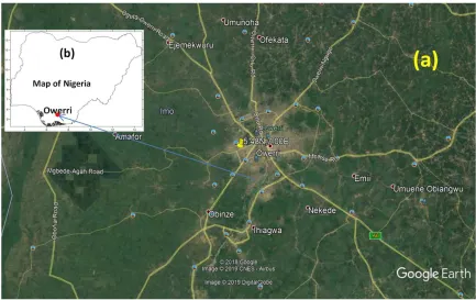
2. Study Area
(Inter-Tropical Convergence Zone). An average annual temperature above 20°C (68.0°F) creates an annual relative humidity of 75%, with humidity reaching 90% in the rainy season [30]. The dry season experiences two months of Harmattan from late December to late February. January and March are the hottest months [30].
Imo state has three main political zones; this are, Okigwe
(Imo North), Orlu (Imo West) and Owerri (Imo East). According to Okorie [31], the state has a population of about 3, 927, 563 with male, 1, 976, 471 and female 1, 951, 092. The state is blessed with natural resources which include, crude oil, natural gas, lead and zinc. Economically exploitable flora like the iroko, mahogany, obeche, bamboo, rubber tree and oil palm predominate [30].
Figure 1. Map of (a) Google map showing the study area (b) Map of Nigeria showing the study area.
3. Methodology
The monthly average minimum temperature, maximum temperature and relative humidity meteorological data used in this study were obtained from the European Centre for Medium-Range Weather Forecasts (ECMWF) at 2m height for owerri, Imo state located in the South Eastern, Nigeria during the period of sixteen years (2000-2015).
Smith [32] developed a correlation between precipitable water and dew point temperature. The coefficients in this correlation vary with latitude and season. Atwater and Ball [33] simplified Smith [32] correlation to
`= exp (0.07074 + ) (1)
where ` is in centimeters, is the station’s dew-point temperature in degrees Celsius and = −0.02290 from April to June and 0.02023 for the remaining months.
For all seasons, Won [34] has developed a simple correlation as follows
`= 0.1 exp (2.2572 + 0.05454 ) (2)
The precipitable water as obtained from Equations (1) and (2) applies to prevailing station pressure and temperature. However, the attenuation equations often require this
quantity to be reduced to a datum of 1013.25 mbars pressure and 273 K temperature. Paltridge and Platt [35] suggest the following formula for reduction of ` to the datum conditions:
= `
!"!#.$%& # '( $)#
* & ! $(
(3)
where w is the reduced precipitable water in centimeters, p is station pressure in millibars, and T is the surface (dry-bulb) temperature in degrees Kelvin.
Leckner [36] has presented the following formula, which expresses precipitable water in terms of relative humidity:
=".'+# ,- .
* (4)
where /0 is relative humidity in fractions of one, is ambient temperature in degrees Kelvin and 12 is the partial pressure of water vapour in saturated air and is given by the semi empirical equation as
12= exp (26.23 −%'!5* ) (5)
The dew point temperature ( ) was obtained using [37] as:
= − 6(!""789)% : (6)
where and ;< are the mean temperature and relative humidity in degree Celsius and percentage respectively.
The Virtual temperature ( = 0 > ) was obtained using the expression [29] as
= 0 > =!7?*
@(!7A) (7)
where B is water vapour pressure and C is a constant given as C = 0.622
The Potential temperature ( ) was obtained using the expression [29] as
= D E&8 F(@ (8)
Equation (8) is called Poisson’s equation, where 1" is a standard pressure generally taken as 1000 hPa and ; G( = 0.286.
The virtual temperature ( =F) correction is given by [29] as.
=F= = 0 > − D (9)
The dew point depression ( 0 22 ) is given by [29] as.
0 22 = D − (10)
In this paper, the skewness and kurtosis tests were studied. The skewness test (IJ) measures the asymmetry of the
parameters data around their mean value; it is a measure of symmetry, or more precisely, the lack of symmetry [38]. It gives information about the direction of variation of the dataset [38]. If IJ= 0, the data have a Gaussian distribution (normal distribution), while IJ< 0 indicates that the data are spread out more to the left of the mean value than to its right (negatively skewed), when IJ > 0 signifies that data are spread out more to the right than to its left (positively skewed) [39].
The Kurtosis test (M>) explains the shape of a random variable’s probability distribution, that is it characterizes the relative peakedness or flatness of a distribution compared to the normal distribution [38]. It measures the degree of normality of each of the meteorological parameters under investigation [39]. For M>= 0 the data have normal distribution, for M>> 0 the data have positive kurtosis which connotes peaked distribution, that is, leptokurtic distribution (that is, too tall), when M>< 0 the data have negative kurtosis which implies flat distribution, that is, platykurtic distribution (that is, too flat, or even concave if the value is large enough).
4. Results and Discussion
The result in figure 2 revealed that; the Smith’s model increases from its minimum value of 3.436 cm in the month of January to March and slightly decreases in April and then increases to July and decreases with a dip downward in the month of August and then increases to its maximum value of 4.807 cm in the month of September and drop subsequently to December.
Figure 2. Monthly variation of Precipitable Water Vapour Models at Owerri, Nigeria.
The Won’s model increases from its minimum value of 2.401 cm in the month of January and attained its maximum value of 3.135 cm in June and then decreases to August and
slightly increases to September and drop subsequently to December.
The Leckner’s model increases gradually from its
Feb Apr Jun Aug Oct Dec
2.4 2.6 2.8 3.0 3.2 3.4 3.6 3.8 4.0 4.2 4.4 4.6 4.8 5.0
P
re
c
ip
it
a
b
le
W
a
te
r
V
a
p
o
u
r
(c
m
)
Months of the year
minimum value of 3.253 cm in the month of January and attained its maximum value of 4.662 cm in the month of June and then decreases to August and slightly increases to September and drop subsequently to December.
The result of the Won’s model showed that the precipitable water vapour are far away from the other models; however, the Leckner’s model slightly overestimated the Smith’s
model in the months of April, May and June. The Leckner’s precipitable water vapour model is found in between the two models and was reported most suitable model for estimating precipitable water vapour for the study area, since statistical test for validation was not carried out. The conclusion drawn from this as to which model is most suitable for PWV estimation is in conformity with the study analyzed in [40].
Figure 3. Monthly variation of Dew Point Temperature with Precipitable Water Vapour at Owerri, Nigeria.
Figure 3 shows the variation of dew point temperature with precipitable water vapour for the location under investigation. The dew point temperature and precipitable water vapour increases from their minimum value of 18.061°C and 3.253 cm in the month of January and attained their maximum value of 22.879°C and 4.662 cm in the month of June and decreases from June to August with a dip downward; though the dew point temperature is more
conspicuous. The dew point temperature and precipitable water vapour increases to September and drop to December. The result indicated high and low values of dew point temperature and precipitable water vapour during the raining and dry seasons respectively. The result further showed that the dew point temperature is a reflection of the precipitable water vapour.
Figure 4. Monthly variation of Dew Point Temperature with Relative Humidity at Owerri, Nigeria.
Figure 4 shows the variation of dew point temperature with relative humidity for the location under investigation.
Feb Apr Jun Aug Oct Dec
1 2 3 4 5
Leckner T
dew
Months of the year
L e c k n e r' s p re c ip it a b le w a te r (c m ) 18 20 22 24 D e w p o in t t e m p e ra tu re ( 0 C )
Feb Apr Jun Aug Oct Dec
54 56 58 60 62 64 66 68 70 72 74 76 78 80 82 84 86 88 90
92 RH Tdew
Months of the year
The relative humidity increases from its minimum value of 56.243% in the month of January to 89.002% in July and then decreases slightly in the month of August and increases to its maximum value of 89.453% in September and drop subsequently to December. The dew point temperature follows similar pattern of variation except that its minimum value of 18.061°C was observed in the month of January and
maximum value of 22.879°C in the month of June; the decrease in the value of dew point temperature begins from July while for relative humidity is from August. High and low values of dew point temperature and relative humidity were observed during the raining and dry seasons respectively. The result of this study revealed that the dew point temperature is a reflection of relative humidity.
Figure 5. Monthly variation of Tdew, Tvirtual, Tpotential and Tmean for Owerri, Nigeria.
Figure 5 shows the monthly variation of dew point temperature, virtual temperature, potential temperature and mean temperature for the location under investigation. The result revealed that the virtual temperature is greater than the dew point temperature, potential temperature and mean temperature while the dew point temperature has the lowest value. The potential temperature and mean temperature follows similar pattern of variation and the virtual temperature follows almost similar pattern of variation; the virtual temperature, potential temperature and mean temperature increases slightly from January to March and decreases from March to July and maintain almost a constant value from July to September and increases from September to December while the virtual temperature decreases slightly from November to December. On the other hand, the dew point temperature increases from it minimum value of 18.061°C in the month of January and attained its maximum value of 22.879°C in the month of June and decreases from June to August with a dip downward and then increases to September and drop to December. The result of this study
showed high values of virtual temperature, potential temperature and mean temperature during the dry season and low values during the raining season while for the dew point temperature high values were recorded during the raining season and low values during the dry seasons; this shows that the dew point temperature is an opposite reflection of the virtual temperature, potential temperature and mean temperature. Considering the dew point temperature and the mean temperature; the dew point temperature increases with increase in mean temperature from January to March and decreases with decrease in mean temperature in the month of July for the location under investigation. The result indicated that the dew point temperature is always less than the mean/air temperature which implies that mean temperature cannot be lower than the dew point temperature; this helps meteorologists predict temperature lows in a weather forecast. The moderate values of the dew point temperature signifies the stability of air for the study area and less tendency of development of thunderstorms as very high dew point temperature can bring about severe weather condition.
Table 1. Monthly average virtual temperature correction and dew point depression for Owerri, Nigeria.
Month Tdew (°C) Tvirtual (°C) Tpotential (°C) Tmean (°C) Tvc (°C) Tdepression (°C)
JAN 18.0611 29.1496 27.6106 26.8125 2.3371 8.7514
FEB 20.196 30.4729 28.5771 27.7219 2.751 7.5259
MAR 21.1418 30.7715 28.6814 27.8125 2.959 6.6708
APR 21.5848 30.3427 28.1172 27.2719 3.0709 5.6871
MAY 22.3406 29.9304 27.4276 26.6969 3.2335 4.3563
JUN 22.8794 28.8996 26.1501 25.575 3.3246 2.6956
Feb Apr Jun Aug Oct Dec
18 19 20 21 22 23 24 25 26 27 28 29 30 31
T
e
m
p
e
ra
tu
re
(
0 C
)
Months of the year
Month Tdew (°C) Tvirtual (°C) Tpotential (°C) Tmean (°C) Tvc (°C) Tdepression (°C)
JUL 22.6129 28.0658 25.3269 24.8125 3.2533 2.1996
AUG 22.4121 27.9845 25.2998 24.7688 3.2158 2.3566
SEP 22.7375 28.1267 25.4255 24.8469 3.2798 2.1094
OCT 22.3973 28.7847 26.2327 25.5500 3.2347 3.1528
NOV 21.5740 29.6792 27.3792 26.6031 3.0761 5.0291
DEC 18.7168 29.2391 27.5460 26.7625 2.4766 8.0458
Average 21.3878 29.2872 26.9812 26.2695 3.0177 4.8817
The maximum and minimum virtual temperature correction of 3.3246°C and 2.3371°C was obtained in the months of June and January with an average value of 3.0177°C. The maximum and minimum dew point depression of 8.7514°C and 2.1094°C was obtained in the months of January and September with an average value of 4.8817°C. The result
shows that the maximum and minimum dew point depression and virtual temperature correction occurred in the month of January. The average dew point temperature, virtual temperature, potential temperature and mean temperature are 21.3878°C, 29.2872°C, 26.9812°C and 26.2695°C respectively for Owerri during the period under investigation.
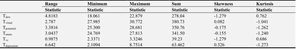
Table 2. Descriptive statistical analysis for the estimated parameters for Owerri, Nigeria.
Range Minimum Maximum Sum Skewness Kurtosis Statistic Statistic Statistic Statistic Statistic Statistic
Tdew 4.8183 18.061 22.879 278.04 -1.279 0.762
Tvitual 2.787 27.985 30.772 380.73 0.082 -1.041
Tpotential 3.3816 25.300 28.681 350.76 -0.175 -1.262
Tmean 3.0437 24.769 27.813 341.50 -0.155 -1.240
Tvc 0.9875 2.3371 3.3246 39.23 -1.279 0.686
Tdepression 6.642 2.1094 8.7514 63.462 0.326 -1.273
The results shown in Table 2 showed that the dew point temperature, potential temperature, mean temperature and virtual temperature correction data spread out more to the left of their mean value (negatively skewed), while the virtual temperature and dew point depression data spread out more to the right of their mean value (positively skewed). The virtual temperature, potential temperature, mean temperature and dew point depression data seem to have a quassi-Gaussian distribution. Skewness of exactly zero is quite not likely for real world data [38]. The dew point temperature and virtual temperature correction data are more divergent away from the normal distribution. It is clear from Table 2 that the dew point temperature and the virtual temperature correction data have positive kurtosis which indicates a relatively peaked distribution and possibility of a leptokurtic distribution. The virtual temperature, potential temperature, mean temperature and dew point depression data have negative kurtosis which indicates a relatively flat distribution and possibility of platykurtic distribution.
5. Conclusion
This study presents the distribution of monthly mean Precipitable water vapour (PWV) based on three models, the Smith; Won; and the Leckner’s model using meteorological parameters of monthly mean temperature and relative humidity obtained from the European Centre for Medium-Range Weather Forecasts (ECMWF) at 2m height for Owerri, Imo state located in the South Eastern, Nigeria during the period of sixteen years (2000-2015). The distribution of PWV showed clear differences; the Smith (ranging from 3.436 to 4.807 cm); Won (ranging from 2.401 to 3.135 cm) and the Leckner’s model (ranging from 3.253 to 3.135 cm). The highest PWV occurred in June for Won and Leckner’s
depression data have negative kurtosis which indicates a relatively flat distribution and possibility of platykurtic distribution for the location under investigation.
Acknowledgements
The authors wish to thank the European Centre for Medium-Range Weather Forecasts (ECMWF) for providing all the necessary meteorological data used in this study. The contribution and suggestions of the anonymous reviewers is well appreciated.
References
[1] Held, I. M and Soden, B. J (2000). Water vapor feedback and global warming, Annual Review of Environment and Resources. vol. 25, pp. 441-475.
[2] Trenberth, K. E., Fasullo, J and Smith, L (2005). Trends and variability in column-integrated atmospheric water vapor. Climate Dynamics, vol. 24, no. 7-8, pp. 741-758.
[3] Wang, J., Carlson, D. J., Parsons, D. B et al (2003). Performance of operational radiosonde humidity sensors in direct comparison with a chilled mirror dew-point hygrometer and its climate implication. Geophysical Research Letters. vol. 30, no. 16.
[4] Wagner, T., Beirle, S., Grzegorski, M et al (2006). Global trends (1996-2003) of total column precipitable water observed by Global Ozone Monitoring Experiment (GOME) on ERS 2 and their relation to near-surface temperature. Journal of Geophysical Research: Atmospheres. vol. 111, no. 12, Article IDD12102.
[5] Dai, A (2006). Recent climatology, variability, and trends in global surface humidity,” Journal of Climate. vol. 19, no. 15: pp. 3589- 3606.
[6] Dai, A., Wang, J., Thorne, P. W et al (2011). A new approach to homogenize daily radiosonde humidity data. Journal of Climate. vol. 24, no. 4: pp. 965-991.
[7] Zhao, T., Dai, A and Wang, J (2012). Trends in tropospheric humidity from 1970 to 2008 over china from a homogenized radiosonde dataset. Journal of Climate. vol. 25, no. 13: pp. 4549-4567.
[8] Mieruch, S., No¨el, S., Bovensmann, H et al (2008). Analysis of global water vapour trends from satellite measurements in the visible spectral range. Atmospheric Chemistry and Physics. vol. 8, no. 3, pp. 491-504.
[9] Zhang, L., Wu, L and Gan, B (2013). Modes and mechanisms of global water vapor variability over the twentieth century. Journal ofClimate. vol. 26, no. 15, pp. 5578-5593 USA. [10] Peng, W., Tongchuan, X., Jiageng, D et al (2017). Trends and
Variability in Precipitable Water Vapor throughout North China from 1979 to 2015. Hindawi Advances in Meteorology. Volume 2017, Article ID 7804823, PP 1-10.
[11] Kiehl, J. T and Trenberth, K. E (1997). Earth’s Annual Global Mean Energy Budget. Bull Am Meteorol Soc. 78: 197-208. [12] Adeyemi, B (2009). Empirical Formulations for Inter-Layer
Precipitable Water Vapor in Nigeria. The Pacific Journal of
Science and Technology. Volume 10, Number 2: Pp 35-45. [13] Dupont, J. C., Haeffelin, M., Drobinski, P et al (2008).
Parametric model to estimate clear-sky long wave irradiance at the surface on the basis of vertical distribution of humidity and temperature. J. Geophys. Res. 113, D07203. http://dx.doi.org/10.1029/2007JD009046
[14] Lanzante, J. R., Klein, S. A and Seidel, D. J (2003). Temporal homogenization of monthly radiosonde temperature data. Part II: Methodology. J. Climate 16: 224-240.
[15] Gerding, M., Christoph, R., Marion, M et al (2004). Tropospheric water vapour soundings by lidar at high Arctic latitudes. Atmos. Res. 71 (4), 289-302.
[16] Kuwahara, T., Mizuno, A., Nagahama, T et al (2008). Groundbased millimeter-wave observations of water vapor emission (183 GHz) at Atacama. Chile. Adv. Space Res. 42 (7): 1167-1171.
[17] Eng, R. S., Kelley, P. L., Mooradian, A et al (1973). Tunable laser measurements of water vapor transitions in the vicinity of 5 lm. Chem. Phys. Lett. 19 (15), 524-528.
[18] Bevis, M., Businger, S., Herring, T. A et al (1992). GPS meteorology. Remote sensing of atmospheric water vapour using the Global Positioning System. J. Geophys. Res. 97: 15784-15801.
[19] Hagemann, S., Bengtsson, L and Gendt, G (2003). On the determination of atmospheric water vapor from GPS measurements. J. Geophys. Res., 4678.
[20] Li, G., Kimura, F., Sato, T et al (2008). A composite analysis of diurnal cycle of GPS precipitable water vapor in central Japan during Calm Summer Days. Theoret. Appl. Climatol. 92 (1/2): 15.
[21] Stoew, B., Elgered, G., Johansson, J. M (2001). An assessment of estimates of integrated water vapor from ground-based GPS data. Meteorol. Atmos. Phys. 77, 99-107. [22] Pramualsakdikul, S., Haas, R., Elgered, G et al (2007).
Sensing of diurnal and semi diurnal variability in the water vapour content in the tropics using GPS measurements. Meteorol. Appl. 14, 403-412.
[23] Maghrabi, A and Al Dajani, H. M (2013). Estimation of precipitable water vapour using vapour pressure and air temperature in an arid region in central Saudi Arabia. Journal of the Association of Arab Universities for Basic and Applied Sciences. 14, 1-8.
[24] Dee, D. P., Uppala, S. M., Simmons, A. J et al (2011). The ERA-Interim reanalysis: configuration and performance of the data assimilation system. Quarterly Journal of the Royal Meteorological Society. vol. 137, no. 656, pp. 553-597. [25] Easterling, D. R and Peterson, T. C (1995). A new method for
detecting undocumented discontinuities in climatological time series. International Journal of Climatology. vol. 15, no. 4: pp. 369-377.
[26] Raymond, A. S (1991). College physics. Saunders College Publishing, Harrisonburg, Virginia.
[28] Moss, M (2016). Capitol broadcasting company. Raleigh, North Carolina, USA; 2016.
[29] Wallace, J. M and Hobbs, P. V (2006). Atmospheric Science, An Introductory Survey, 2nd Edition, Elsevier, pp 66-82. [30] Okorie, F. C., Okeke, I., Nnaji, A et al (2012). Evidence of
Climate Variability in Imo State of Southeastern Nigeria. Journal of Earth Science and Engineering. 2 (2012) 544-553. [31] Okorie, F. C (2010). Great Ogberuru in Its Contemporary
Geography, Cape Publishers, Owerri, Nigeria.
[32] Smith, W (1966). Note on the relationship between total precipitable water and surface dew point. J. Appl. Meteorol. 5, 726-727.
[33] Atwater, M. A and Ball, J. T (1976). Comparisons of radiation computations using observed and estimated precipitable water. Appl. Meteorol. 15: 1319-1320.
[34] Won, T (1977). The simulation of hourly global radiation from hourly reported meteorological parameters Canadian Prairie Area. Conference, 3rd, Canadian Solar Energy Society Inc., Radiative Processes in Meteorology and Climatology. American Elsevier, New York.
[35] Paltridge, G. W and Platt, C. M. R (1976). Radiative Processes in Meteorology and Climatology. American Elsevier, New York, 1976.
[36] Leckner, B (1978). The spectral distribution of solar radiation at the earth's surface—elements of a model. Sol Energy 20 (2), 143-150.
[37] Lawrence, M. G (2005). The relationship between relative humidity and the dewpoint temperature in moist air: A simple conversion and applications. Bull. Amer. Meteor. Soc., 86, 225-233. doi: http;//dx.doi.org/10.1175/BAMS-86-2-225. [38] Akpootu, D. O., Iliyasu, M. I., Mustapha, W et al (2017). The
Influence of Meteorological Parameters on Atmospheric Visibility over Ikeja, Nigeria. Archives of Current Research International. 9 (3): 1-12. doi: 10.9734/ACRI/2017/36010. [39] Hejase, H. A. N and Assi, A. H (2011). Time-Series
Regression Model for Prediction of Monthly and Daily Average Global Solar Radiation in Al Ain City-UAE. Proceedings of the Global Conference on Global Warming held on 11-14 July, 2011, Lisbon, Portugal. Pp 1-11.