Statistical Characterization of Extreme Hydrologic Parameters for the Peripheral River System of Dhaka City

(1)

Journal of Water Resources and Ocean Science

2014; 3(3): 30-37

Published online July 20, 2014 (http://www.sciencepublishinggroup.com/j/wros) doi: 10.11648/j.wros.20140303.11

ISSN: 2328-7969 (Print); ISSN: 2328-7993 (Online)

Statistical characterization of extreme hydrologic

parameters for the peripheral river system of Dhaka city

Sarfaraz Alam

*

, Muhammad Sabbir Mostafa Khan

Department of Water Resources Engineering, Bangladesh University of Engineering and Technology, Dhaka 1000, Bangladesh

Email address:

sarfaraz@wre.buet.ac.bd (S. Alam), mostafakhan@wre.buet.ac.bd (M. S. M. Khan)

To cite this article:

Sarfaraz Alam, Muhammad Sabbir Mostafa Khan. Statistical Characterization of Extreme Hydrologic Parameters for the Peripheral River System of Dhaka City.Journal of Water Resources and Ocean Science. Vol. 3, No. 3, 2014, pp. 30-37. doi: 10.11648/j.wros.20140303.11

Abstract:

Selection of appropriate probability distribution function is one of the most important steps of frequency analysis. Due to the existence of large number of distributions, hydrologists follow different methods to select the best one. In this paper, annual maximum, minimum water level and discharge of five peripheral rivers, namely Buriganga, Turag, Tongi, Balu and Lakhya around Dhaka city have been analyzed to compute the basic statistics and fit them with sixty two probability density functions (PDF). Three goodness-of-fit (GoF) statistics, namely Chi-square, Kolmogorov–Smirnov and Anderson Darling were used to rank each of the distribution. Furthermore, ranks obtained from three GoF were used to compute overall rank of all distributions for each hydrologic parameter. The study reveals that, four different distributions were found best fit for four extreme cases. Dagum (4P) and Chi-square (2P) fit best for annual maximum and minimum water level respectively, whereas Cauchy and Johnson SB were found for annual maximum and minimum discharge respectively. Moreover, ranks of frequently used distributions, namely General Extreme Value (GEV), Log-Pearson III (LP3), Log-normal (LN) and Gumbels were compared with the best fit distributions and did not give satisfactory results. The method used in this study would be helpful for flood frequency analysis of other rivers of Bangladesh. This may also be used for evaluation of best fit distribution of river system for other countries as well.

Keywords:

Probability Distribution, Rank, Water Level, Discharge, Dhaka City

1. Introduction

Design of different types of hydraulic structures and flood plain zoning, economic evaluation of flood protection projects, etc. require information on flood magnitudes and their frequencies (Rakesh 2005). In addition low flow frequency analysis is also required for assessing water quality, water availability, navigability etc. Moreover climate change associated with global warming got potentiality to change the probability of these events. In particular, highly populated cities surrounded by rivers are vulnerable to flooding and pollution. Urban development and industrialization demand good estimation of both water level and discharge. Thus, it is necessary to explore the water level and discharge extremes around major cities, especially which are in highly populated regions dominated by socio-economic development and prone to pollution and flooding.

Reliable flood frequency distribution selection is one of the major problems faced by the hydrologists. This issue is

(2)

parameter estimation methods, such as method maximum likelihood and probability (Betül Saf 2009). Different goodness-of as Chi-square, Kolmogorov–Smirnov Darling may also show different ranks distribution.

A number of studies have been conducted of Bangladesh using frequently used distribution Ferdows M (2005) compared three

distributions, namely Log Normal (Two and three parameters, LN3); Extreme value Grumbel and Log-person type-3 (LP3), flow of three major rivers (Meghna, Ganges-5 stations). In Bangladesh, four mainly used for at-sit frequency analysis maximum discharge. Gumbel and LN distribution by Bangladesh Water Development

departments/ firms respectively, whereas were used in National Water Plan and respectively (Karim MA and Chowdhury MA and Chowdhury JA. (1995) suggested for flood frequency analysis of the rivers Bari MF. et al.(2002) found that LP3 low flow frequency analysis for the rivers Bangladesh. So, almost all the researches flow were conducted using frequently used

In this study an attempt has been made best distributions for annual maximum, level and discharge. The study area is located most densely populated region in the capital city of Bangladesh is surrounded rivers, namely Buriganga, Turag, Balu, Annual maximum, minimum water level of these rivers were used to compute the fit them with sixty two distributions. Three (GoF) statistics, namely Chi-square, Kolmogorov and Anderson Darling were used to rank

Furthermore, median of the ranks obtained for each distribution were used to compute

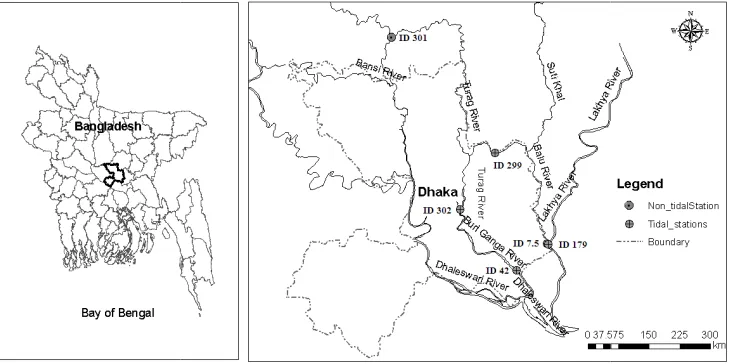
Figure 1. (a)

method of moments, probability-weighted-moments of- fit statistics, such Smirnov and Anderson ranks for each type of

conducted on the rivers distribution functions. three frequently used (Two parameters, LN2 value Type-l (EVl) or (LP3), using annual peak (Meghna, Brahmaputra, four distributions are analysis of annual distribution are used Development Board and few whereas LP3 and GEV and Flood Action Plan Chowdhury JA. 1995). Karim suggested the use of GEV rivers of Bangladesh. is more suitable for rivers in North-West researches on low and high used distributions.

made to identify the maximum, minimum water located at one of the the world. Dhaka, the surrounded by a number of Balu, Lakhya and Tongi. level and discharge data the basic statistics and Three goodness-of-fit Kolmogorov–Smirnov rank each distribution. obtained from three GoF compute overall rank of

all PDFs for each extreme hydrologic Table 5 shows the ranks for annual Top three distributions for each dataset were finally computed. distributions, namely GEV, LP3, shown to assess their performance extreme cases.

2. Study Region and

2.1. Study Region

Dhaka city is highly populated rapid socio-economic growth. km2 with an estimated growth labeled the city as a mega Harada, 2001; Rahman S. and above MSL is 4 m. Buriganga, Lakhya are the peripheral river as shown in Fig 1. The area monsoon rainfall leading to Considerable attention has occurrence of flood of different

2.2. Data Collection

Yearly maximum, minimum and discharge for 3 stations Bangladesh Water Development of the gauging stations can be information of the dataset is one station on Turag river all tidal flow.

3. Methodology

In this research sixty functions (PDF) were used to and discharge dataset. The list Table 2.

(a) Bangladesh map (b) Peripheral river system of Dhaka city (right).

hydrologic parameter, likewise annual maximum water level . each station and each type of computed. Ranks of frequently used LP3, LN and Gumbels are also performance for different hydrologic

and Data

populated and influenced by the growth. The area of the city is 360 growth rate of 4.2% per annum that city (Haigh, 2004; Karn and and Hossain, F., 2007). Elevation Buriganga, Turag, Balu, Tongi and river system around Dhaka city area is greatly affected by the to flood and water logging. been paid to understand the different return period.

minimum water level for 6 stations stations were collected from Development Board (BWDB). Location be referred to Fig 1. Detailed given in Table 1. Other than all the stations are subjected to

one probability distribution to fit the observed water level list of PDF’s used are given in

(3)

Journal of Water Resources and Ocean Science 2014; 3(3): 30-37 32

Table 1. Dataset of water level and discharge station location

Station id Station Longitude Latitude River Type Time interval

301 Kaloikor 90.210 24.082 Turag Non Tidal WL & Q 1949-2009

42 Dhaka (Mill Barak) 90.445 23.677 Buriganga Tidal WL 1909-2009

302 Mirpur 90.338 23.783 Turag Tidal WL 1954-2009

299 Tongi Khal 90.404 23.882 Tongi Tidal WL 1960-2009

179 Demra 90.505 23.723 Lakhya Tidal WL & Q 1952-2009

7.5 Demra 90.502 23.723 Balu Tidal WL & Q 1962-2009

Table 2. Probability density functions used for fitting all hydrological dataset.

Beta Burr Burr (4P) Cauchy Chi-Squared Chi-Squared (2P) Dagum Dagum (4P)

Erlang Erlang (3P), Error Error Function Exponential Exponential (2P), Fatigue Life Fatigue Life

(3P)

Frechet Frechet (3P) Gamma Gamma (3P) Gen. Extreme

Value Gen. Gamma

Gen. Gamma

(4P) Gen. Pareto

Gumbel

Max Gumbel Min Hypersecant Inv. Gaussian

Inv. Gaussian

(3P) Johnson SB Kumaraswamy Laplace

Lognormal Lognormal (3P) Nakagami Normal Pareto Pareto 2 Pearson 5 Pearson 5

(3P)

Pearson 6 Pearson6 (4P) Pert Power Function Rayleigh Rayleigh (2P) Reciprocal Rice

Student's t Triangular Uniform Weibull Weibull(3P) Johnson SU Levy Levy(2P)

Log-Gamma Log-Logistic Log-Logistic(3P) Log-Pearson 3 Log-Normal

For each station annual maximum, minimum water level and discharge were plotted using all the distributions above (few were found not applicable in some cases). Goodness

of fit was performed using Chi-Square,

Kolmogorov-Smirnov and Anderson Darling. Ranks according to these three goodness of fit showed a great variation. Median of the ranks obtained from goodness of fit for each PDF was used to rank all the PDFs. A sample example is given in Table 3 showing ranks of maximum water level of Turag river at station 301. PDF’s such as General Extreme Value (GEV), Log Pearson Type III, Log Normal and Gumbels which are mostly used for extreme value analysis are shown in Table 3 to highlight their ranking. All the distributions were fitted and ranked using the tool Easyfit. Three goodness of fit method gave separate ranking for each PDF. Median of the ranks obtained from three GoF for each distribution was used to compute the overall rank of all the PDFs. This procedure was followed for maximum, minimum water level and discharge for each station. Finally all these ranks were used to obtain the best fit distributions for each extreme hydrologic parameter. A sample example for station 301 (Turag) is shown in Table 9 (Appendix) which illustrates the best fit distributions obtained following the above procedure. Best fit distributions found from different GoF statistic and median of the ranks for station 301 are shown in Fig 2.

4. Results and Discussion

4.1. Basic Statistics

In order to understand the statistical properties of annual maximum and minimum water level and discharge of the peripheral rivers of Dhaka city, basic statistics have been computed (Table 3-4). We have described descriptive statistics such as max, min, range, min, variance, standard

(4)

Whereas lowest mean and standard deviation were computed at station 301, though it possess highest coefficient of variation of 1.04 and excess kurtosis 14.77. Considering all discharge dataset it was found that discharge variation is highest at station 301 (2200-0.42 m3/s), standard deviation also varied greatly (462.94 to 3.26) at this station. Station 179 has a tendency to show negative skewness which is opposite to others. So, considering all the annual water level dataset highest variation (10.48-0.49) and standard deviation (1.78, 0.56) are associated with station 301 which is non tidal in behavior. Most of the stations showed negative skewness while annual maximum WL considered, whereas the scenario was vice versa considering annual minimum WL. Other than one case (Annual minimum WL, station 301 = -0.76) all the stations showed positive excess kurtosis.

a)

b)

c)

d)

e)

Figure 2. Probability density function plotting of station 301 for annual maximum WL a) Best 3 based on the median of ranks obtained from Goodness-of-fits b) Frequently used distributions c) Best 3 according to Kolmogorov Smirnov d) Best 3 according to Anderson Darling e) Best 3 according to Chi-Squared

Table 3. Descriptive statistics of annual water level (mPWD) for individual stations

Station Id River Max Min N Range Mean Variance Std. Dev Coeff. of variation Std. error Skewness Excess Kartosis Annual Max. Water Level (mPWD)

301 Turag 10.48 2.27 60 8.21 7.7 3.18 1.78 0.23 0.23 -1.8 3.38

42 Buriganga 7.58 3.2 94 4.38 5.77 0.38 0.62 0.11 0.06 -0.37 3.12

302 Turag 8.35 2.71 54 5.64 6.18 0.9 0.95 0.15 0.13 -0.63 2.57

299 Tongi 7.84 2.71 49 5.13 5.99 0.88 0.94 0.16 0.13 -1.34 4.01

179 Lakhya 7.11 4.56 48 2.55 5.84 0.25 0.50 0.09 0.07 0.39 0.69

7.5 Balu 7.09 2.57 46 4.52 5.82 0.47 0.69 0.12 0.10 -2.19 10.47

Annual Min. Water Level (mPWD)

301 Turag 2.91 0.49 60 2.42 1.66 0.31 0.56 0.34 0.07 -0.17 -0.76

42 Buriganga 1.23 0.24 95 0.99 0.66 0.03 0.16 0.25 0.02 0.48 1.82

302 Turag 1.71 0.12 56 1.59 0.80 0.06 0.24 0.29 0.03 0.64 3.64

299 Tongi 1.52 0.53 50 0.99 0.94 0.04 0.20 0.21 0.03 0.86 1.15

179 Lakhya 1.42 0.48 49 0.94 0.84 0.03 0.16 0.20 0.02 0.98 2.83

(5)

Table 4. Descriptive statistics of discharge(m3_{/s) for individual stations}

Station Id River Max Min N Range Mean Variance Std. Dev Coeff. of

variation Std. error Skewness Excess Kartosis

Annual Max. Discharge (m3_/s)

301 Turag 2200 4 32 2196 686.11 214320 462.94 0.67 81.84 0.91 2.58

179 Lakhya 2610 774 26 1935.8 1947.3 143210 378.44 0.19 74.22 -1.35 4.3

7.5 Balu 2077.3 140 21 1937.3 451.47 167850 409.69 0.91 89.4 3.52 13.53

Annual Min. Discharge (m3_/s)

301 Turag 18.2 0.42 32 17.78 3.14 10.64 3.26 1.04 0.58 3.38 14.77

179 Lakhya 1300 106 26 1194 647.24 100450 316.94 0.49 62.16 -0.02 -0.81

7.5 Balu 288.52 16.1 21 272.42 73.33 4214.9 64.92 0.89 14.17 2.13 5.38

Table 5. Best fit distributions and ranks of GEV, Log Pearson III, Log Normal and Gumbels for annual maximum water level.

St. id Best 3 distributions Ranks of mostly used PDF

#1 #2 #3 GEV Log Pearson III Log Normal Gumbels

Annual Max. water level

301 Cauchy Dagum (4P) Weibull (3P) 25 31 41 34

42 Burr (4P) Hypersecant Dagum 11 46 29 28

302 Hypersecant Log-logistic Laplace 28 47 29 35

299 Log logistic (3P) Laplace Dagum(4P) 27 50 35 30

179 Dagum Burr Log-Logistic 25 11 14 44

7.5 Cauchy Dagum(4P) Log logistic (3P) 29 52 34 28

All Dagum (4P) Log-Logistic (3P) Burr (4P) 24 30 46 31

Table 6. Best fit distributions and ranks of GEV, Log Pearson III, Log Normal and Gumbels for annual minimum water level.

Annual Min. water level

301 Dagum(4P) Gen. Gamma Error 10 29 16 28

42 Laplace Erlang Hypersecant 14 33 34 41

302 Dagum(4P) Log-logistic Burr 8 7 14 34

299 Chi-squared Burr (4P) Chi-squared(2P) 17 11 19 43

179 Cauchy Chi-squared(2P) Chi-squared 24 21 17 44

7.5 Chi-squared(2P) Log logistic (3P) Logistics 13 48 34 32

All Chi-Squared (2P) Burr (4P) Chi-Squared 10 28 16 42

Table 7. Best fit distributions and ranks of GEV, Log Pearson III, Log Normal and Gumbels for annual maximum discharge.

Max. Discharge

301 Error Hypersecant Laplace 10 27 45 16

179 Cauchy Log-logistic(3P) Laplace 20 40 23 29

7.5 Cauchy Burr Log-logistic(3P) 19 31 12 19

All Cauchy Laplace Log-Logistic (3P) 17 36 25 18

Table 8. Best fit distributions and ranks of GEV, Log Pearson III, Log Normal and Gumbels for annual minimum discharge.

Min. Discharge

301 Fatigue Life Logistic Log Normal (3P) 8 7 32 47

179 Dagum Error Johnson AB 4 10 40 19

7.5 Gen. Pareto Johnson AB Fatigue Life (3P) 4 12 2 52

(6)

4.2. Ranking of Probability Distribution Function

All the PDF were ranked for both water level and discharge at each station. Finally all those ranks were used to determine the ranking of PDF for similar type of dataset, such as max. wl, min. wl, max. Q and min. Q. Table 5-8 describes best three distributions for each type of dataset, ranks of mostly used distributions are also added in those tables.

Best fit distributions for annual maximum water level are listed in Table 5. It reveals great combination of various types of distributions. Considering all dataset Dagum(4P), Log-logistic(3P) and Burr (4P) were found the best three. On the other hand ranks of frequently used distributions GEV, LP3, LN and Gumbels were 24, 30, 46 and 31 respectively. Similarly, ranks of distributions for minimum WL are listed in Table 6. Frequently used distributions fell behind in this case too. The ranks obtained are 10, 28, 16 and 42 respectively. Whereas the best fit distributions are Chi-squared (2P), Burr (4P) and Chi-Squared.

Similar to water level, discharge dataset were also fitted to different distributions (Table 7-8). In case of annual maximum discharge various distributions were found best fit for different stations. Frequently used distributions didn’t show good performance in this case. Ranks of frequently used distributions GEV, LP3, LN and Gumbels were 17, 36, 25 and 18 respectively. Best fit distributions were Cauchy, Laplace and Log-logistic (3P). Whereas, considering annual minimum discharge GEV (Generalized Extreme Value) gave a good result in combined ranking. But separately each station gave different best fit distributions. Best fit distributions for annual minimum water level were Johnson SB, GEV and Inv. Gaussian (3P).

5. Conclusion

In this study annual maximum, minimum water level and discharge of the peripheral river system of Dhaka city have been analyzed to identify the best fit distribution among sixty two distributions. Three goodness-of-fit statistics (GoF), namely Chi-square, Kolmogorov-Smirnov and Anderson Darling were used to rank all distributions median of the ranks obtained from three GoF for each distribution were used to compute overall rank of all PDFs for each extreme hydrologic parameter. The study reveals that, four different distributions were found best fit for four extreme hydrologic cases. Dagum (4P) and Chi-square (2P) fit best for annual maximum and minimum water level respectively, whereas Cauchy and Johnson SB were found for annual maximum and minimum discharge respectively. The ranks of frequently used distributions GEV, LP3, LN and Gumbels were not satisfactory for almost all the hydrologic parameters.

Recommendation

The method used in this study would be helpful for flood frequency analysis of other rivers of Bangladesh. This may also be used for evaluation of best fit distribution for other countries as well.

Acknowledgements

Authors are gratefully acknowledging the cooperation rendered by Bangladesh Water Development Board (BWDB) for providing the necessary data.

Appendix

Table 9. Ranking of PDF for maximum water level of Turag river at Kaloikor station (st. id 301)

Distribution

Kolmogorov Smirnov Ranking of PDF for maximum water

level of Turag river at Kaloikor station (st. id 301) Anderson Darling Chi-Squared Median

Statistic Rank Statistic Rank Statistic Rank Value Rank

Beta 0.15 10 1.69 7 11.00 15 10 9

Burr 0.16 12 2.78 13 11.09 16 13 13

Burr (4P) 0.11 5 1.20 6 4.12 3 5 4

Cauchy 0.09 1 0.61 1 0.79 1 1 1

Chi-Squared 0.42 51 13.42 47 85.33 53 51 53

Chi-Squared (2P) 0.37 50 10.98 43 70.84 51 50 51

Dagum 0.16 11 1.87 9 13.21 19 11 10

Dagum (4P) 0.10 3 0.97 2 10.52 14 3 2

Erlang 0.29 42 8.43 37 23.58 37 37 36

Erlang (3P) 0.22 28 4.39 21 16.77 31 28 27

Error 0.19 18 2.73 12 8.36 10 12 12

Error Function 0.92 59 554.77 60 932.97 54 59 59

Exponential 0.47 53 17.66 51 22.18 34 51 53

(7)

Distribution

Kolmogorov Smirnov Ranking of PDF for maximum water

level of Turag river at Kaloikor station (st. id 301) Anderson Darling Chi-Squared Median

Statistic Rank Statistic Rank Statistic Rank Value Rank

Fatigue Life 0.31 44 8.52 38 37.72 43 43 42

Fatigue Life (3P) 0.21 25 3.96 19 16.46 26 25 22

Frechet 0.37 49 12.13 45 67.57 50 49 49

Frechet (3P) 0.28 40 7.57 34 25.91 38 38 38

Gamma 0.23 30 6.18 29 13.27 20 29 28

Gamma (3P) 0.21 26 4.40 22 17.30 32 26 24

Gen. Extreme Value 0.13 8 12.53 46 N/A 27 25

Gen. Gamma 0.26 38 6.63 31 28.76 40 38 38

Gen. Gamma (4P) 0.12 7 1.12 3 6.06 7 7 7

Gen. Pareto 0.18 16 33.68 58 N/A 37 36

Gumbel Max 0.26 36 11.84 44 16.73 30 36 34

Gumbel Min 0.14 9 1.71 8 8.17 8 8 8

Hypersecant 0.18 15 2.91 14 11.65 17 15 15

Inv. Gaussian 0.20 23 7.23 33 15.92 22 23 19

Inv. Gaussian (3P) 0.20 22 3.88 17 16.45 25 22 18

Johnson SB 0.18 14 19.27 53 N/A 33.5 33

Kumaraswamy 0.12 6 1.20 5 4.12 5 5 4

Laplace 0.19 19 2.73 11 8.36 11 11 10

Levy 0.58 57 22.39 55 36.62 42 55 57

Levy (2P) 0.49 56 16.29 50 1.48 2 50 51

Log-Gamma 0.31 45 9.64 40 38.01 44 44 45

Log-Logistic 0.30 43 8.20 36 47.62 47 43 42

Log-Logistic (3P) 0.10 2 1.97 10 5.54 6 6 6

Log-Pearson 3 0.18 17 14.32 48 N/A 32.5 31

Logistic 0.19 20 3.19 16 16.54 27 20 16

Lognormal 0.29 41 7.86 35 35.34 41 41 41

Lognormal (3P) 0.21 27 4.25 20 16.71 28 27 25

Nakagami 0.17 13 5.07 26 10.46 13 13 13

Normal 0.21 24 3.94 18 16.45 24 24 20

Pareto 0.49 55 19.40 54 8.25 9 54 56

Pareto 2 0.48 54 18.33 52 22.45 35 52 55

Pearson 5 0.32 46 9.51 39 50.62 48 46 46

Pearson 5 (3P) 0.24 33 5.02 25 14.06 21 25 22

Pearson 6 0.27 39 7.15 32 41.17 45 39 40

Pearson 6 (4P) 0.25 34 5.25 28 20.05 33 33 32

Pert 0.19 21 3.01 15 16.25 23 21 17

Power Function 0.22 29 4.74 24 12.12 18 24 20

Rayleigh 0.32 47 9.95 42 78.45 52 47 48

Rayleigh (2P) 0.35 48 9.64 41 47.13 46 46 46

Reciprocal 0.58 58 32.26 57 27.50 39 57 58

Rice 0.25 35 5.15 27 16.73 29 29 28

Student's t 0.92 60 208.24 59 1199.10 55 59 59

Triangular 0.26 37 4.69 23 22.68 36 36 34

Uniform 0.24 31 22.66 56 N/A 43.5 44

Weibull 0.24 32 6.53 30 55.19 49 32 30

Weibull (3P) 0.11 4 1.19 4 4.12 4 4 3

(8)

References

[1] Bari MF and Sadek S., Regionalization of low-flow frequency estimates for rivers in northwest Bangladesh, FRIEND 2002—Regional Hydrology: Bridging the Gap between Research and Practice (Proceedings of the fourth International FRIEND Conference held at Cape Town. South Africa. March 2002). IAHS Publ. no. 274.

[2] Betül Saf (2009), Regional Flood Frequency Analysis Using L-Moments for the West Mediterranean Region of Turkey , Water Resour Manage 23:531–551 DOI 10.1007/s11269-008-9287-z

[3] Bobee B, Cavidas G, Ashkar F, Bernier J, Rasmussen P (1993) Towards a systematic approach to comparing distributions used in flood frequency analysis. J Hydrol 142:121–136 [4] Coulson CH (1991) Manual of operational hydrology in B.C.,

2nd edn. B.C. Water Management Division, Hydrology Section, Ministry of Environment, Lands and Parks, BC, Canada

[5] Cunanne C (1973) A particular comparison of annual maxima and partial duration series methods of flood frequency prediction. J Hydrol 18:257–271

[6] Cunnane C (1989) Statistical distributions for flood frequency analysis. WMO No. 718, WMP, Geneva

[7] Ferdows M and Hossain M (2005), Flood Frequency Analysis at Different Rivers in Bangladesh: A Comparison Study on Probabilitv Distribution Functions, Thammasat Int. J. Sc. Tech., Vol. 10, No. 3, 53-62

[8] Haddad K. and Rahman A. (2010). Selection of the best fit flood frequency distribution and parameter estimation procedure: a case study for Tasmania in Australia, Stoch Environ Res Risk Assess (2011) 25, DOI 10.1007/s00477-010-0412-1, 415–428

[9] Haigh M.J. (2004). Sustainable management of headwater resources: the Nairobi ‘headwater’ declaration (2002) and beyond. Asian Journal of Water, Environment and Pollution, Vol. 1, No. 1-2, 17–28.

[10] Karn S.K. and Harada, H. (2001). Surface water pollution in three urban territories of Nepal, India, and Bangladesh. Environmental Management, Vol. 28, No. 4, 483–496 [11] Karim MA and Chowdhury JA. (1995) A comparison of four

distributions used in flood frequency analysis in Bangladesh, Hydrological Sciences Journal, 40:1, 55-66, DOI: 10.1080/02626669509491390

[12] Laio F, Di Baldassarre G, Montanari A (2009) Model selection techniques for the frequency analysis of hydrological extremes. Water Resour Res 45:W07416. doi:10.1029/2007/WR006666

[13] Markiewicz I, Strupczewski WG, Kochanek K, Singh V (2006) Discussion of Non-stationary pooled flood frequency analysis. J Hydrol 276:210–223

[14] Mitosek HT, Strupczewski WG, Singh VP (2006) Three procedures for selection of annual flood peak distribution. J Hydrol 323: 57–73

[15] Rahman AS., Rahman A., Zaman MA., Haddad K., Ahsan A., Imteaz M. (2013), A study on selection of probability distributions for at-site flood frequency analysis in Australia, Nat Hazards (2013) 69:1803–1813 DOI

10.1007/s11069-013-0775-y

[16] Rahman S. and Hossain, F., (2007). Spatial Assessment of Water Quality in Peripheral Rivers of Dhaka City for Optimal Relocation of Water Intake Point. Water Resources Management, Vol. 1, No. 22, 377-391.

[17] Rakesh Kumar and Chandranath Chatterjee,(2005), Regional Flood Frequency Analysis Using L-Moments for North Brahmaputra Region of India, J. Hydrol. Eng, ASCE, Vol. 10, No. 1, 1-7, DOI:10.1061/(ASCE)1084-0699(2005)10:1(1) [18] Stedinger JR (1980) Fitting lognormal distributions to

hydrologic data. Water Resour Res 16(3):481–490

[19] Stedinger JR, Vogel RM, Foufoula-Georgiou E (1992) Frequency analysis of extreme events. In: Maidment DR (ed) Handbook of hydrology. McGraw-Hill, New York